跳到论文正文
W Papers独立论文阅读器 arXiv:1505.00769 论文正文 计算阅读时间 · 0%
引用这篇论文根据当前论文元数据生成,正式投稿前建议核对。


License: arXiv.org perpetual non-exclusive license
arXiv:1505.00769v2 [cs.IT] 09 Apr 2016

On Non-Interactive Simulation of Joint Distributions

Sudeep Kamath1, Venkat Anantharam2 ††thanks: Part of this paper was presented at the 50th Annual Allerton Conference on Communications, Control and Computing 2012, Monticello, Illinois. This document is the final version of the paper to appear in the IEEE Transactions on Information Theory. Affiliation:  Affiliation: 1ECE Department, Princeton University,
sukamath@princeton.edu
Affiliation:  Affiliation: 2EECS Department, University of California, Berkeley,
ananth@eecs.berkeley.edu
August 24, 2026
Abstract

We consider the following non-interactive simulation problem: Alice and Bob observe sequences XnX^{n} and YnY^{n} respectively where {(Xi,Yi)}i=1n\{(X_{i},Y_{i})\}_{i=1}^{n} are drawn i.i.d. from P⁡(x,y),P(x,y), and they output UU and VV respectively which is required to have a joint law that is close in total variation to a specified Q⁡(u,v).Q(u,v). It is known that the maximal correlation of UU and VV must necessarily be no bigger than that of XX and YY if this is to be possible. Our main contribution is to bring hypercontractivity to bear as a tool on this problem. In particular, we show that if P⁡(x,y)P(x,y) is the doubly symmetric binary source, then hypercontractivity provides stronger impossibility results than maximal correlation. Finally, we extend these tools to provide impossibility results for the kk-agent version of this problem.

I Introduction

The problem of simulating random variables by two agents with suitable resource constraints has had a rich history leading to different formulations of this problem in the literature. The general setup for the problem is as follows: Two or more agents wish to simulate a specified joint distribution under resource constraints in the form of limited communication, limited common randomness provided to all of them, or limited correlation between their observations. One then wishes to find the minimum resources required to achieve the desired goal.

The simulation problem has natural applications in numerous areas — from game-theoretic co-ordination in a network against an adversary to control of a dynamical system over a distributed network. These problems are expected to be important in many future technologies with remote-controlled applications, such as Amazon’s drone-based delivery system [1] and robotic environmental cleanup, vegetation management, land clearing, and bio-mass harvesting [2]. In these technologies, individual robotic components would need to take randomized actions under limited or no communication with other components or the central system. Study of the simulation problem can provide fundamental limits on the capabilities of such robotic components and guide efficient usage of the available resources.

The earliest studied two-agent simulation problems were considered by Gács and Körner [3], and Wyner [4]. One may interpret their results, which we will describe shortly, in the framework of a generalization of both their problem setups as shown in Fig. 1. Let the random variables X,Y,U,VX,Y,U,V shown take values in finite sets.

Refer to caption
Fig. 1: A generalization of the problem setups considered by Gács-Körner [3] and Wyner[4]

In this formulation, two agents each having access to its own infinite stream of private randomness, observe nn i.i.d. copies of samples generated according to a specified law P⁡(x,y)P(x,y) as shown, and are required to output n​RnR samples drawn from a distribution that is close (in total variation) to the the distribution constructed by taking i.i.d. copies of a specified law Q⁡(u,v).Q(u,v). Let the simulation capacity R∗R^{*} be defined as the supremum of all rates for which given any ϵ>0,\epsilon>0, it is possible for some nn to carry out this task to within total variation distance ϵ\epsilon.

  • •

    When Q⁡(u,v)Q(u,v) is described by U=V∼Ber⁡(1/2),U=V\sim\Ber(1/2), and P⁡(x,y)P(x,y) is a general distribution, this problem considers fundamental limits for extracting common randomness from the distribution of (X,Y).(X,Y). Gács and Körner showed in [3] that we have the simulation capacity R∗=K⁡(X,Y),R^{*}=K(X;Y), which has come to be known as the Gács-Körner common information of XX and Y.Y. This quantity K⁡(X,Y)K(X;Y) can be described as supH⁡(Θ)\sup H(\Theta) where Θ=f⁡(X)=g⁡(Y).\Theta=f(X)=g(Y). In other words, the simulation capacity is non-zero only when the distribution of (X,Y)(X,Y) is decomposable, i.e. 𝒳\mathcal{X} may be partitioned as 𝒳1∪𝒳2\mathcal{X}_{1}\cup\mathcal{X}_{2} and 𝒴\mathcal{Y} may be partitioned as 𝒴1∪𝒴2\mathcal{Y}_{1}\cup\mathcal{Y}_{2} so that 𝖯𝗋⁡(X∈𝒳1,Y∈𝒴2)=𝖯𝗋⁡(X∈𝒳2,Y∈𝒴1)=0\mathsf{Pr}\left(X\in\mathcal{X}_{1},Y\in\mathcal{Y}_{2}\right)=\mathsf{Pr}\left(X\in\mathcal{X}_{2},Y\in\mathcal{Y}_{1}\right)=0 and 𝖯𝗋⁡(X∈𝒳1,Y∈𝒴1),𝖯𝗋⁡(X∈𝒳2,Y∈𝒴2)>0.\mathsf{Pr}\left(X\in\mathcal{X}_{1},Y\in\mathcal{Y}_{1}\right),\mathsf{Pr}\left(X\in\mathcal{X}_{2},Y\in\mathcal{Y}_{2}\right)>0. Further, they showed that in general, K⁡(X,Y)≤I⁡(X,Y).K(X;Y)\leq I(X;Y).

  • •

    When P⁡(x,y)P(x,y) is described by X=Y∼Ber⁡(1/2),X=Y\sim\Ber(1/2), and Q⁡(u,v)Q(u,v) is a general distribution, this problem considers fundamental limits for common randomness needed for generating the random variable pair (U,V)(U,V). Wyner showed in [4] that the amount of common information needed for generation per sample is (R∗)−1=C⁡(U,V),(R^{*})^{-1}=C(U;V), which has come to be known as the Wyner common information of UU and V.V. This quantity C⁡(U,V)C(U;V) can be described as supI⁡(Θ,U,V)\sup I(\Theta;U,V) over all Θ\Theta satisfying U−Θ−VU-\Theta-V with cardinality bound on the variable Θ\Theta given by |Θ|≤|𝒰|⋅|𝒱|.|\mathsf{\Theta}|\leq|\mathcal{U}|\cdot|\mathcal{V}|. Further, Wyner showed that C⁡(U,V)≥I⁡(U,V)C(U;V)\geq I(U;V) in general. To be precise, Wyner considered a problem setting that required (U,V)(U,V) to be simulated with vanishing normalized relative entropy, i.e. if Q′​(un​R,vn​R)Q^{\prime}(u^{nR},v^{nR}) is the law of the simulated samples, and Q⁡(u,v)Q(u,v) was the target distribution, then simulation is considered possible in Wyner’s formulation if

    1n​RD(Q′(un​R,vn​R)||Πi=1n​RQ(ui,vi))→0.\displaystyle\frac{1}{nR}D\left(Q^{\prime}(u^{nR},v^{nR})||\Pi_{i=1}^{nR}Q(u_{i},v_{i})\right)\to 0. (1)

    It has been recognized that the simulation capacity remains the same under the vanishing total variation constraint [5, Lemma 5], [6, Lemma IV.1]. A recent work [7] considers a variant of Wyner’s problem with exact generation of random variables as opposed to generation with a vanishing total variation distance.

The problem of characterizing R∗R^{*} is open for general distributions P⁡(x,y)P(x,y) and Q⁡(u,v),Q(u,v), and so is the problem of characterizing when R∗>0.R^{*}>0.

In another stream of related work, the problem of simulation has been considered under rate-limited interaction between the agents. This began with the work of Cuff [8] who studied communication requirements for simulating a channel with rate-limited communication and rate-limited common randomness. [9] studied communication requirements for establishing dependence among nodes in a network setting. The former setup (of Cuff [8]) was generalized by Gohari and Anantharam in [10] (see Fig. 2). Two agents wish to simulate i.i.d. samples of a specified joint distribution P⁡(x,y,u,v).P(x,y,u,v). Nature supplies i.i.d. copies of (X,Y)(X,Y) with the right marginal distribution as shown and the agents can use a certain rate of common randomness, certain rate-limited communication, and infinite streams of individual private randomness to accomplish the desired task. We want to understand the fundamental trade-offs between these rates to make this task possible. This problem was completely solved by Yassaee, Gohari, and Aref in [11]. However, this work does not address the problem of computing the simulation capacity R∗R^{*} for the setup in Fig. 1, since the problem formulation there is different in two respects: In Fig. 2, the task is to output nn samples while in Fig. 1, the task is to output n​RnR samples. Furthermore, even if RR were say chosen to be 1, in Fig. 2, the joint distribution of the quadruple (Xn,Yn,Un,Vn)(X^{n},Y^{n},U^{n},V^{n}) is required to be close to i.i.d. copies of a specified joint distribution. However, in Fig. 1, the requirement is only on the marginal distribution of the output samples (Un,Vn)(U^{n},V^{n}) and the quadruple (Xn,Yn,Un,Vn)(X^{n},Y^{n},U^{n},V^{n}) need not even be close to an i.i.d. distribution.

Refer to caption
Fig. 2: Generalization of Cuff’s formulation [8] by Gohari and Anantharam [10]

In this paper, we consider the former non-interactive simulation setup à la Gács-Körner and Wyner (Fig. 1). Since the problem of characterizing whether R∗>0R^{*}>0 for general distributions P⁡(x,y)P(x,y) and Q⁡(u,v),Q(u,v), is also non-trivial, we propose a relaxed problem where two agents observe an arbitrary finite number of samples drawn i.i.d. from P⁡(x,y)P(x,y) as shown in Fig. 3 and are required to output one random variable each with the requirement that the output distribution be close in total variation to a specified Q⁡(u,v).Q(u,v). Clearly, if it is impossible to generate even a single sample, we must have R∗=0.R^{*}=0. We therefore focus on impossibility results for this problem which will be relevant to the formulation in Fig. 1. It is not clear if the converse is true, i.e. it is unclear whether the feasibility of generating one sample asymptotically implies that we may generate samples at a rate R>0.R>0.

Note that the notion of simulation we consider is distinct from the notion of exact generation wherein a certain distribution is required to be generated exactly. If we have a strategic setting, such as a distributed game, in which a player, represented by a number of distributed agents, is playing against an adversary, the agents would often need to generate a joint distribution exactly [12], to avoid providing unforeseen strategic advantages to the adversary.

Refer to caption
Fig. 3: The non-interactive simulation problem considered in this paper

When (U,V)∼Q⁡(u,v)(U,V)\sim Q(u,v) is described by U=V∼Ber⁡(1/2)U=V\sim\Ber(1/2) while P⁡(x,y)P(x,y) is a general distribution, the problem has recently come to be called non-interactive correlation distillation [13, 14]. We therefore, call our formulation the problem of non-interactive simulation of joint distributions. In a remarkable strengthening of the Gács-Körner result [3], Witsenhausen showed in [15] that unless the Gács-Körner common information K⁡(X,Y)K(X;Y) is positive (i.e. the joint distribution of (X,Y)(X,Y) is decomposable), non-interactive correlation distillation is impossible to achieve. The chief tool used in Witsenhausen’s proof is the maximal correlation of two random variables, a quantity which will be of prime importance in the present paper as well.

The second tool that we will be using is hypercontractivity, which has found numerous applications in mathematics, physics, and theoretical computer science. The origins of hypercontractivity lie in the early works of Bonami [16, 17], of Nelson [18] in quantum field theory, of Gross [19] who first developed the connection to logarithmic Sobolev inequalities, and of Beckner [20]. The meaning of hypercontractivity was broadened by Borell [21] to what is sometimes called reverse hypercontractivity today [22]. Hypercontractivity has found powerful applications in a lot of fields, for example the study of influence of variables on Boolean functions [23], [24], [25] and in voting system theory[26]. Ahlswede and Gács [27] identified the use of hypercontractivity in studying the spreading of sets in high dimensional product spaces. In recent works, [28] showed an equivalence between hypercontractivity and strong data processing inequalities for Rényi divergences, [29] used hypercontractivity to show non-vanishing lower bounds on hypothesis testing, [30] studied hypercontractivity for a noise operator that computed spherical averages in Hamming space, [31] showed a connection between hypercontractivity and strong data processing inequalities for mutual information, and [32] used hypercontractivity to study the mutual information between Boolean functions. As we shall see, hypercontractivity has properties that make it naturally well-suited for studying the non-interactive simulation problem.

Let us formally set up the non-interactive simulation problem described earlier.

Definition 1.

Let 𝒳,𝒴,𝒰,𝒱\mathcal{X},\mathcal{Y},\mathcal{U},\mathcal{V} denote finite sets. Given a source distribution P⁡(x,y)P(x,y) over 𝒳×𝒴\mathcal{X}\times\mathcal{Y} and a target distribution Q⁡(u,v)Q(u,v) over 𝒰×𝒱,\mathcal{U}\times\mathcal{V}, we say that non-interactive simulation of Q⁡(u,v)Q(u,v) using P⁡(x,y)P(x,y) is possible, if for any ϵ>0,\epsilon>0, there exists a positive integer n,n, a finite set ℛ,\mathcal{R}, and functions f:𝒳n×ℛ↦𝒰,f:\mathcal{X}^{n}\times\mathcal{R}\mapsto\mathcal{U}, g:𝒴n×ℛ↦𝒱g:\mathcal{Y}^{n}\times\mathcal{R}\mapsto\mathcal{V} such that

dTV​((f⁡(Xn,MX),g⁡(Yn,MY)),(U,V))≤ϵd_{\mathrm{TV}}\left((f(X^{n},M_{X}),g(Y^{n},M_{Y}));(U,V)\right)\leq\epsilon

where {(Xi,Yi)}i=1n\{(X_{i},Y_{i})\}_{i=1}^{n} is a sequence of i.i.d. samples drawn from P⁡(x,y),P(x,y), MX,MYM_{X},M_{Y} are uniformly distributed in ℛ\mathcal{R} and are mutually independent of each other and the samples from the source, (U,V)(U,V) is drawn from Q⁡(u,v)Q(u,v) and dTV​(⋅,⋅)d_{\mathrm{TV}}(\cdot\,;\cdot) is the total variation distance (defined as half the L1L_{1} distance between the distributions).

For a fixed P⁡(x,y),P(x,y), the set of distributions Q⁡(u,v)Q(u,v) on a fixed set 𝒰×𝒱\mathcal{U}\times\mathcal{V} for which non-interactive simulation is possible is precisely the closure of the set of marginal distributions of (U,V)(U,V) satisfying U−Xk−Yk−VU-X^{k}-Y^{k}-V for some k.k. However, this set of distributions appears to be very hard to characterize explicitly. In this paper, we focus on outer bounds on this set, or in other words impossibility results for non-interactive simulation.

Note that since we are interested only in determining the possibility of simulation and not in the simulation capacity, the problem does not have any less generality if we disallow the agents from using any private randomness, since agents can obtain as much private randomness as desired by using extended observations that are non-overlapping in time, i.e. the agents observe n1+n2+n3n_{1}+n_{2}+n_{3} symbols, they use (X1,…,Xn1),(Y1,…,Yn1)(X_{1},\ldots,X_{n_{1}}),(Y_{1},\ldots,Y_{n_{1}}) respectively as their correlated observations, Alice uses Xn1+1,…,Xn2X_{n_{1}+1},\ldots,X_{n_{2}} as her private randomness, and Bob uses Yn2+1,…,Yn3Y_{n_{2}+1},\ldots,Y_{n_{3}} as his private randomness. We make the choice to assume the availability of private randomness as part of the model.

We will consider two examples to motivate the focus of this study.

I-A Example 1

Let XX be a uniform Bernoulli random variable, X∼Ber⁡(12).X\sim\Ber(\frac{1}{2}). Let YY be a noisy copy of X,X, i.e. Y=X+NY=X+N where N∼Ber⁡(α)N\sim\Ber(\alpha) for 0<α<12,0<\alpha<\frac{1}{2}, is independent of X.X. Here, the addition is modulo 2. We say that (X,Y)(X,Y) has the doubly symmetric binary source distribution with parameter α,\alpha, denoted DSBS⁡(α)\DSBS(\alpha) following the notation of Wyner [4]. We consider (U,V)∼DSBS⁡(β)(U,V)\sim\DSBS(\beta) for 0≤β<12.0\leq\beta<\frac{1}{2}. We may ask whether non-interactive simulation of Q⁡(u,v)=DSBS⁡(β)Q(u,v)=\DSBS(\beta) using P⁡(x,y)=DSBS⁡(α)P(x,y)=\DSBS(\alpha) is possible. Witsenhausen answered this question in the negative when β<α\beta<\alpha in [15], thus significantly strengthening the result of Gács and Körner [3]. Witsenhausen established this by proving the tensorization of the maximal correlation of an arbitrary pair of random variables (both tensorization and maximal correlation are defined and discussed in Section II-A). This can be used to conclude that if non-interactive simulation is possible, then the maximal correlation of the target distribution can be no more than that of the source distribution. The parameter nn has disappeared in this comparison thanks to the tensorization property. The maximal correlation of a pair of binary random variables distributed as DSBS⁡(α)\DSBS(\alpha) equals |1−2​α|.|1-2\alpha|. Thus, for instance, if the non-interactive simulation of DSBS⁡(β)\DSBS(\beta) using DSBS⁡(α)\DSBS(\alpha) is possible, with 0≤α,β≤12,0\leq\alpha,\beta\leq\frac{1}{2}, then we must have α≤β.\alpha\leq\beta. Furthermore, it is easy to see that if α≤β,\alpha\leq\beta, then non-interactive simulation is indeed possible: Alice outputs the first bit of her observation while Bob outputs a suitable noisy copy of his first bit. Thus, for 0≤α,β≤12,0\leq\alpha,\beta\leq\frac{1}{2}, non-interactive simulation of DSBS⁡(β)\DSBS(\beta) using DSBS⁡(α)\DSBS(\alpha) is possible if and only if α≤β.\alpha\leq\beta.

I-B Example 2

Let P⁡(x,y)P(x,y) be given by (X,Y)∼DSBS⁡(α)(X,Y)\sim\DSBS(\alpha) with 0<α<12.0<\alpha<\frac{1}{2}. Consider binary random variables (U,V)(U,V) distributed as Q⁡(u,v)Q(u,v) given by: Q⁡(0,0)=0,Q⁡(0,1)=Q⁡(1,0)=Q⁡(1,1)=13.Q(0,0)=0,Q(0,1)=Q(1,0)=Q(1,1)=\frac{1}{3}. We ask if non-interactive simulation of Q⁡(u,v)Q(u,v) using DSBS⁡(α)\DSBS(\alpha) is possible. The maximal correlation of a DSBS⁡(α)\DSBS(\alpha) source distribution is |1−2​α||1-2\alpha| while that of Q⁡(u,v)Q(u,v) is 12.\frac{1}{2}. Since non-interactive simulation is impossible unless the maximal correlation of the source exceeds that of the target, we have non-interactive simulation impossible if |1−2​α|≤12,|1-2\alpha|\leq\frac{1}{2}, i.e. 14<α<12.\frac{1}{4}<\alpha<\frac{1}{2}. But what about the case when 0<α≤14​?0<\alpha\leq\frac{1}{4}? Can we come up with a suitable scheme to simulate Q⁡(u,v)Q(u,v)? The answer turns out to be no for each 0<α≤140<\alpha\leq\frac{1}{4} and can be proved using the following inequality which holds for {(Xi,Yi)}i=1n\{(X_{i},Y_{i})\}_{i=1}^{n} being i.i.d. DSBS⁡(α),\DSBS(\alpha), and for arbitrary sets S,T⊆{0,1}n:S,T\subseteq\{0,1\}^{n}:

𝖯𝗋⁡(Xn∈S,Yn∈T)≥𝖯𝗋​(Xn∈S)12​α​𝖯𝗋​(Yn∈T)12​α.\mathsf{Pr}\left(X^{n}\in S,Y^{n}\in T\right)\geq\mathsf{Pr}\left(X^{n}\in S\right)^{\frac{1}{2\alpha}}\mathsf{Pr}\left(Y^{n}\in T\right)^{\frac{1}{2\alpha}}. (2)

The above inequality follows from a so-called reverse hypercontractive inequality [13, Thm. 3.4]. We will revisit this inequality in Section II-C. If non-interactive simulation of Q⁡(u,v)Q(u,v) using DSBS⁡(α)\DSBS(\alpha) were possible, we should be able to find sets S,TS,T such that 𝖯𝗋⁡(Xn∈S)≈13,𝖯𝗋⁡(Yn∈T)≈13\mathsf{Pr}\left(X^{n}\in S\right)\approx\frac{1}{3},\mathsf{Pr}\left(Y^{n}\in T\right)\approx\frac{1}{3} and 𝖯𝗋⁡(Xn∈S,Yn∈T)≈0.\mathsf{Pr}\left(X^{n}\in S,Y^{n}\in T\right)\approx 0. Inequality (2) rules out this possibility (assuming private randomness is not available, which we had argued is without loss of generality). Thus, hypercontractivity or reverse hypercontractivity can provide impossibility results when the maximal correlation approach cannot. Is it true that one is always stronger than the other? One of the main results in our paper is that hypercontractivity allows for stronger impossibility results than the maximal correlation when P⁡(x,y)=DSBS⁡(α).P(x,y)=\DSBS(\alpha). More generally, we give necessary and sufficient conditions on P⁡(x,y)P(x,y) for this subsumption. This arises from an inequality obtained by Ahlswede and Gács[27] in the hypercontractive case which we extend to the reverse hypercontractive case.

The rest of the paper is organized as follows. Section II discusses preliminaries on maximal correlation and hypercontractivity. We present our main results in Section III. As mentioned earlier, one of our main results is a necessary and sufficient condition on the source distribution P⁡(x,y)P(x,y) which allows one to definitively conclude that hypercontractivity will provide stronger impossibility results than maximal correlation. As our second main result, we give a characterization of a limiting hypercontractivity parameter (that we call s∗s^{*}) as a strong data processing constant for KL divergences. This characterization was first proven by Ahlswede-Gacs [27]. However, our proof has the advantage of being more intuitive - arising naturally from a Taylor series expansion - while at the same time extending immediately to reverse hypercontractivity. This hypercontractivity parameter has recently been shown to also be the tightest constant in strong data processing inequalities for mutual information [31]. Section IV discusses the extension of the non-interactive simulation problem for k≥3k\geq 3 agents. We provide a couple of interesting three-user non-interactive simulation examples where every two agents can simulate the corresponding pairwise marginal of the desired joint distribution but the triple cannot simulate the triple joint distribution.

II Main Tools: Maximal Correlation and Hypercontractivity

In this paper, all sets are finite and all probability distributions are discrete and have finite support. We denote the marginals of P⁡(x,y)P(x,y) and Q⁡(u,v)Q(u,v) by PX​(x),PY​(y)P_{X}(x),P_{Y}(y) and QU​(u),QV​(v)Q_{U}(u),Q_{V}(v) respectively. We will use ℝ≥0\mathbb{R}_{\geq 0} and ℝ>0\mathbb{R}_{>0} to denote non-negative reals and strictly positive reals respectively. In the following subsections, we will review the definition and properties of maximal correlation and hypercontractivity.

II-A Maximal Correlation

For jointly distributed random variables (X,Y),(X,Y), define their maximal correlation ρm​(X,Y):=sup𝔼​f​(X)​g​(Y)\rho_{m}(X;Y):=\sup\mathbb{E}f(X)g(Y) where the supremum is taken over f:𝒳↦ℝ,g:𝒴↦ℝf:\mathcal{X}\mapsto\mathbb{R},g:\mathcal{Y}\mapsto\mathbb{R} such that 𝔼​f​(X)=𝔼​g​(Y)=0\mathbb{E}f(X)=\mathbb{E}g(Y)=0 and 𝔼​f​(X)2,𝔼​g​(Y)2≤1.\mathbb{E}f(X)^{2},\mathbb{E}g(Y)^{2}\leq 1.

Example 1.

If (X,Y)∼DSBS⁡(α),(X,Y)\sim\DSBS(\alpha), then the only functions f,gf,g satisfying the conditions 𝔼​f​(X)=𝔼​g​(Y)=0\mathbb{E}f(X)=\mathbb{E}g(Y)=0 and 𝔼​f​(X)2,𝔼​g​(Y)2≤1\mathbb{E}f(X)^{2},\mathbb{E}g(Y)^{2}\leq 1 are f⁡(x)=a⁡(1x=0−1x=1)f(x)=a(1_{x=0}-1_{x=1}) and g⁡(y)=b⁡(1y=0−1y=1)g(y)=b(1_{y=0}-1_{y=1}) with |a|,|b|≤1.|a|,|b|\leq 1. The optimum is then achieved with a=b=1a=b=1 if α<12\alpha<\frac{1}{2} and with a=b=−1a=b=-1 if α≥12.\alpha\geq\frac{1}{2}. Thus,

ρm​(X,Y)=|1−2​α|.\rho_{m}(X;Y)=|1-2\alpha|. (3)

The following properties of the maximal correlation of two discrete random variables with finite support can be shown easily [33].

  1. 1.

    0≤ρm​(X,Y)≤1.0\leq\rho_{m}(X;Y)\leq 1.

  2. 2.

    ρm​(X,Y)=0\rho_{m}(X;Y)=0 if and only if XX is independent of Y.Y.

  3. 3.

    ρm​(X,Y)=1\rho_{m}(X;Y)=1 if and only if the Gács-Körner common information K⁡(X,Y)>0,K(X;Y)>0, i.e. if and only if (X,Y)(X,Y) is decomposable.

The three key properties of maximal correlation that are useful for the non-interactive simulation problem are as follows:

  • •

    (data processing inequality) For any functions ϕ,ψ,\phi,\psi, ρm​(X,Y)≥ρm​(ϕ⁡(X),ψ⁡(Y)).\rho_{m}(X;Y)\geq\rho_{m}(\phi(X),\psi(Y)).

  • •

    (tensorization) If (X1,Y1),(X2,Y2)(X_{1},Y_{1}),(X_{2},Y_{2}) are independent, then ρm​(X1,X2,Y1,Y2)=max⁡{ρm​(X1,Y1),ρm​(X2,Y2)}\rho_{m}(X_{1},X_{2};Y_{1},Y_{2})=\max\{\rho_{m}(X_{1};Y_{1}),\rho_{m}(X_{2};Y_{2})\} [15, Thm. 1].

  • •

    (lower semi-continuity) (Recall that if 𝒰\mathcal{U} is a metric space, uu is a point in 𝒰\mathcal{U} and f:𝒰↦ℝf:\mathcal{U}\mapsto\mathbb{R} is a real-valued function, then we say ff is lower semi-continuous at uu if un→uu_{n}\to u implies lim infnf⁡(un)≥f⁡(u).\liminf_{n}f(u_{n})\geq f(u).) If the space of probability distributions on 𝒳×𝒴\mathcal{X}\times\mathcal{Y} is endowed with the total variation distance metric, then ρm​(X,Y)\rho_{m}(X;Y) is a lower semi-continuous function of the joint distribution P⁡(x,y).P(x,y). [An example will be provided to show that ρm\rho_{m} is not a continuous function of the joint distribution.]

To keep the paper self-contained, proofs of these properties are sketched in Appendix -A. Now, using the above three properties, maximal correlation can be used to prove impossibility results for the non-interactive simulation problem.

Observation 1.

Non-interactive simulation of (U,V)∼Q⁡(u,v)(U,V)\sim Q(u,v) using (X,Y)∼P⁡(x,y)(X,Y)\sim P(x,y) is possible only if ρm​(X,Y)≥ρm​(U,V).\rho_{m}(X;Y)\geq\rho_{m}(U;V).

Proof.

Suppose non-interactive simulation of (U,V)∼Q⁡(u,v)(U,V)\sim Q(u,v) using (X,Y)∼P⁡(x,y)(X,Y)\sim P(x,y) is possible. This means, there exists a sequence of integers (kn:n≥1),(k_{n}:n\geq 1), a sequence of finite alphabets ℛn,\mathcal{R}_{n}, and a sequence of functions fn:𝒳kn×ℛn↦𝒰,f_{n}:\mathcal{X}^{k_{n}}\times\mathcal{R}_{n}\mapsto\mathcal{U}, gn:𝒴kn×ℛn↦𝒱,g_{n}:\mathcal{Y}^{k_{n}}\times\mathcal{R}_{n}\mapsto\mathcal{V}, such that if {Xi,Yi}i=1kn\{X_{i},Y_{i}\}_{i=1}^{k_{n}} are drawn i.i.d. P⁡(x,y)P(x,y) and MX,MYM_{X},M_{Y} are uniformly distributed in ℛn,\mathcal{R}_{n}, with {Xi,Yi}i=1kn,MX,MY\{X_{i},Y_{i}\}_{i=1}^{k_{n}},M_{X},M_{Y} mutually independent, and Un=fn​(Xkn,MX),Vn=gn​(Ykn,MY),U_{n}=f_{n}(X^{k_{n}},M_{X}),V_{n}=g_{n}(Y^{k_{n}},M_{Y}), then dTV​((Un,Vn),(U,V))→0d_{\mathrm{TV}}((U_{n},V_{n});(U,V))\to 0 as n→∞.n\to\infty. We therefore, have

ρm​(Un,Vn)\displaystyle\rho_{m}(U_{n};V_{n}) ≤ρm(Xkn,MX;Ykn,MY) (Data Processing Inequality)\displaystyle\leq\rho_{m}(X^{k_{n}},M_{X};Y^{k_{n}},M_{Y})\mbox{ (Data Processing Inequality)} (4)
=max⁡{ρm​(X1,Y1),ρm​(X2,Y2),…,ρm​(Xkn,Ykn),ρm​(MX,MY)}​ (Tensorization)\displaystyle=\max\{\rho_{m}(X_{1};Y_{1}),\rho_{m}(X_{2};Y_{2}),\ldots,\rho_{m}(X_{k_{n}},Y_{k_{n}}),\rho_{m}(M_{X};M_{Y})\}\mbox{ (Tensorization)} (5)
=max⁡{ρm​(X1,Y1),0}\displaystyle=\max\{\rho_{m}(X_{1};Y_{1}),0\} (6)
=ρm​(X,Y)\displaystyle=\rho_{m}(X;Y) (7)

By lower semi-continuity of ρm\rho_{m}, dTV​((Un,Vn),(U,V))→0d_{\mathrm{TV}}((U_{n},V_{n});(U,V))\to 0 implies

ρm​(U,V)≤lim infn→∞ρm​(Un,Vn)≤ρm​(X,Y).\rho_{m}(U;V)\leq\liminf_{n\to\infty}\rho_{m}(U_{n};V_{n})\leq\rho_{m}(X;Y).

∎

II-B Hypercontractivity

Definition 2.

For any real-valued random variable WW with finite support, and any real number p,p, define

‖W‖p:={(𝔼​|W|p)1/p,p≠0;exp⁡(𝔼​log⁡|W|)p=0,\displaystyle||W||_{p}:=\begin{cases}\left(\mathbb{E}|W|^{p}\right)^{1/p},&p\neq 0;\\ \exp\left(\mathbb{E}\log|W|\right)&p=0,\end{cases} (8)

with the understanding that for p≤0,p\leq 0, ‖W‖p=0||W||_{p}=0 if 𝖯𝗋⁡(|W|=0)>0.\mathsf{Pr}\left(|W|=0\right)>0.

‖W‖p||W||_{p} is continuous and non-decreasing in p.p. If WW is not almost surely a constant, then ‖W‖p||W||_{p} is strictly increasing for p≥0.p\geq 0. If in addition, 𝖯𝗋⁡(|W|=0)=0,\mathsf{Pr}\left(|W|=0\right)=0, then ‖W‖p||W||_{p} is strictly increasing for all p.p.

Definition 3.

For any real p≠0,1,p\neq 0,1, define its Hölder conjugate p′p^{\prime} by 1p+1p′=1.\frac{1}{p}+\frac{1}{p^{\prime}}=1. For p=0,p=0, define p′=0.p^{\prime}=0.

Suppose X,YX,Y are real-valued random variables with finite support. We write X≥0X\geq 0 if 𝖯𝗋⁡(X≥0)=1.\mathsf{Pr}\left(X\geq 0\right)=1. The following are well-known [34]:

  • •

    (Minkowski’s inequality) For p≥1,p\geq 1, ‖X+Y‖p≤‖X‖p+||Y||p.||X+Y||_{p}\leq||X||_{p}+||Y||_{p}.

  • •

    (Reverse Minkowski’s inequality) For p≤1p\leq 1 and X,Y≥0,X,Y\geq 0, ‖X+Y‖p≥‖X‖p+||Y||p.||X+Y||_{p}\geq||X||_{p}+||Y||_{p}.

  • •

    (Hölder’s inequality) For p>1,p>1, 𝔼⁡[X​Y]≤‖X‖p′||Y||p.\mathbb{E}[XY]\leq||X||_{p^{\prime}}||Y||_{p}.

  • •

    (Reverse Hölder’s inequality) For p<1p<1 and X,Y≥0,X,Y\geq 0, 𝔼⁡[X​Y]≥‖X‖p′||Y||p.\mathbb{E}[XY]\geq||X||_{p^{\prime}}||Y||_{p}.

Definition 4.

For a pair of random variables (X,Y)∼P⁡(x,y)(X,Y)\sim P(x,y) on 𝒳×𝒴,\mathcal{X}\times\mathcal{Y}, we say (X,Y)(X,Y) is (p,q)(p,q)-hypercontractive if

  • •

    1≤q≤p,1\leq q\leq p, and

    ‖𝔼⁡[g⁡(Y)|X]‖p≤‖g⁡(Y)‖q∀g:𝒴↦ℝ;||\mathbb{E}[g(Y)|X]||_{p}\leq||g(Y)||_{q}\ \ \forall g:\mathcal{Y}\mapsto\mathbb{R}; (9)

    (If h⁡(Y)=|g⁡(Y)|,h(Y)=|g(Y)|, then −𝔼⁡[h⁡(Y)|X]≤𝔼⁡[g⁡(Y)|X]≤𝔼⁡[h⁡(Y)|X]-\mathbb{E}[h(Y)|X]\leq\mathbb{E}[g(Y)|X]\leq\mathbb{E}[h(Y)|X] pointwise, thus we may equivalently restrict gg to map to ℝ≥0.\mathbb{R}_{\geq 0}. If WnW_{n} supported on at most kk values (for some fixed kk) converges to WW in distribution, then ‖Wn‖p→‖W‖p||W_{n}||_{p}\to||W||_{p} for any p,p, so we may further equivalently restrict gg to map to ℝ>0\mathbb{R}_{>0}.)

  • •

    1≥q≥p,1\geq q\geq p, and

    ‖𝔼⁡[g⁡(Y)|X]‖p≥‖g⁡(Y)‖q∀g:𝒴↦ℝ≥0.||\mathbb{E}[g(Y)|X]||_{p}\geq||g(Y)||_{q}\ \ \forall g:\mathcal{Y}\mapsto\mathbb{R}_{\geq 0}. (10)

    (If WnW_{n} supported on at most kk values (for some fixed kk) converges to WW in distribution, then ‖Wn‖p→‖W‖p||W_{n}||_{p}\to||W||_{p} for any p,p, so we may equivalently restrict gg to map to ℝ>0\mathbb{R}_{>0}.)

Note that in the conventional definitions in (9) and (10), we have functions taking values in ℝ\mathbb{R} and ℝ≥0\mathbb{R}_{\geq 0} respectively. As explained above, for (9), we may restrict to functions taking values in ℝ≥0.\mathbb{R}_{\geq 0}. However, in (10), the functions must take non-negative values. This is conventional and necessary in various“reverse” inequalities such as the reverse Minkowski and reverse Hölder inequalities.

Define the hypercontractivity ribbon ℛ⁡(X,Y)\mathcal{R}(X;Y) as the set of pairs (p,q)(p,q) for which (X,Y)(X,Y) is (p,q)(p,q)-hypercontractive.

It is easy to check that the inequalities (9), (10) always hold for p=q.p=q. The conditional expectation operator is thus always contractive when p≥1,p\geq 1, and reverse contractive for positive-valued functions when p≤1.p\leq 1. For random variables (X,Y)(X,Y) with a specific distribution P⁡(x,y),P(x,y), the operator may be hypercontractive (i.e. more than contractive) in this precise sense. ℛ⁡(X,Y)\mathcal{R}(X;Y) is a region in ℝ2\mathbb{R}^{2} pinching to a point at (1,1)(1,1) resembling a ribbon, explaining our choice of the name (see Fig. 4). Inequality (10) is also referred to as reverse hypercontractivity in the literature [22].

Fig. 4: The hypercontractivity ribbon ℛ⁡(X,Y)\mathcal{R}(X;Y) is the shaded region. Also shown a straight line of slope ρm2:=ρm2​(X,Y)\rho_{m}^{2}:=\rho_{m}^{2}(X;Y) through (1,1)(1,1) (from Thm. 1).

II-B1 Interpretation of hypercontractivity as Hölder-contractivity

It is well-known [22] that an equivalent definition of ℛ⁡(X,Y)\mathcal{R}(X;Y) can be given by observing how much the corresponding Hölder’s and reverse Hölder’s inequalities may be tightened:

  • •

    (1,1)∈ℛ⁡(X,Y);(1,1)\in\mathcal{R}(X;Y);

  • •

    For 1≤q≤p,1<p1\leq q\leq p,1<p we have (p,q)∈ℝ⁡(X,Y)(p,q)\in\mathbb{R}(X;Y) iff

    𝔼​f​(X)​g​(Y)\displaystyle\mathbb{E}f(X)g(Y) ≤‖f⁡(X)‖p′||g⁡(Y)||q∀f:𝒳↦ℝ,g:𝒴→ℝ;\displaystyle\leq||f(X)||_{p^{\prime}}||g(Y)||_{q}\ \ \ \forall f:\mathcal{X}\mapsto\mathbb{R},g:\mathcal{Y}\to\mathbb{R}; (11)
  • •

    For 1≥q≥p,1>p1\geq q\geq p,1>p we have (p,q)∈ℝ⁡(X,Y)(p,q)\in\mathbb{R}(X;Y) iff

    𝔼​f​(X)​g​(Y)\displaystyle\mathbb{E}f(X)g(Y) ≥‖f⁡(X)‖p′||g⁡(Y)||q∀f:𝒳↦ℝ>0,g:𝒴↦ℝ>0;\displaystyle\geq||f(X)||_{p^{\prime}}||g(Y)||_{q}\ \ \forall f:\mathcal{X}\mapsto\mathbb{R}_{>0},g:\mathcal{Y}\mapsto\mathbb{R}_{>0}; (12)

We will refer to inequalities (11), (12) as Hölder-contractive inequalities since they tighten Hölder’s inequality (using the knowledge that XX and YY are not ‘too correlated’ in a suitable sense).

To see the equivalence for 1≥q≥p,1>p1\geq q\geq p,1>p observe that if (10) holds for any strictly positive-valued function g,g, then for any fixed strictly positive-valued function f,f, we have

𝔼​f​(X)​g​(Y)\displaystyle\mathbb{E}f(X)g(Y) =𝔼⁡[f⁡(X)​𝔼​[g⁡(Y)|X]]\displaystyle=\mathbb{E}\left[f(X)\mathbb{E}[g(Y)|X]\right] (13)
≥‖f⁡(X)‖p′||𝔼⁡[g⁡(Y)|X]||p​ (Reverse Hölder’s inequality and 𝔼⁡[g⁡(Y)|X]>0)\displaystyle\geq||f(X)||_{p^{\prime}}||\mathbb{E}[g(Y)|X]||_{p}\mbox{\ \ \ (Reverse H\"{o}lder's inequality and $\mathbb{E}[g(Y)|X]>0$)} (14)
≥‖f⁡(X)‖p′||g⁡(Y)||q.\displaystyle\geq||f(X)||_{p^{\prime}}||g(Y)||_{q}. (15)

Conversely, suppose (12) holds for any strictly positive-valued functions f,g.f,g. First assume p≠0.p\neq 0. By fixing gg and choosing f⁡(X)=𝔼​[g⁡(Y)|X]p−1,f(X)=\mathbb{E}[g(Y)|X]^{p-1}, we get

𝔼⁡[𝔼​[g⁡(Y)|X]p]\displaystyle\mathbb{E}\left[\mathbb{E}[g(Y)|X]^{p}\right] =𝔼⁡[𝔼​[g⁡(Y)|X]p−1​g​(Y)]\displaystyle=\mathbb{E}\left[\mathbb{E}[g(Y)|X]^{p-1}g(Y)\right] (16)
≥‖𝔼​[g⁡(Y)|X]p−1‖p′||g⁡(Y)||q\displaystyle\geq||\mathbb{E}[g(Y)|X]^{p-1}||_{p^{\prime}}||g(Y)||_{q} (17)
=(𝔼⁡[𝔼​[g⁡(Y)|X]p])1−1p||g⁡(Y)||q.\displaystyle=\left(\mathbb{E}\left[\mathbb{E}[g(Y)|X]^{p}\right]\right)^{1-\frac{1}{p}}||g(Y)||_{q}. (18)

Since 𝔼⁡[g⁡(Y)|X]>0,\mathbb{E}[g(Y)|X]>0, we obtain ‖𝔼⁡[g⁡(Y)|X]‖p≥||g⁡(Y)||q.||\mathbb{E}[g(Y)|X]||_{p}\geq||g(Y)||_{q}.

Now, consider the case p=0.p=0. If (12) holds for any strictly positive-valued functions f,gf,g with p=p′=0,p=p^{\prime}=0, then by monotonicity of ||⋅||r||\cdot||_{r} in r,r, we also have

𝔼​f​(X)​g​(Y)\displaystyle\mathbb{E}f(X)g(Y) ≥‖f⁡(X)‖−ϵ||g⁡(Y)||q∀f:𝒳↦ℝ>0,g:𝒴↦ℝ>0;\displaystyle\geq||f(X)||_{-\epsilon}||g(Y)||_{q}\ \ \forall f:\mathcal{X}\mapsto\mathbb{R}_{>0},g:\mathcal{Y}\mapsto\mathbb{R}_{>0}; (19)

By our previous argument, this gives ‖𝔼⁡[g⁡(Y)|X]‖ϵ1+ϵ≥||g⁡(Y)||q.||\mathbb{E}[g(Y)|X]||_{\frac{\epsilon}{1+\epsilon}}\geq||g(Y)||_{q}. Since this holds for each ϵ>0,\epsilon>0, we get from continuity of ||⋅||p||\cdot||_{p} in pp that ‖𝔼⁡[g⁡(Y)|X]‖0≥||g⁡(Y)||q.||\mathbb{E}[g(Y)|X]||_{0}\geq||g(Y)||_{q}.

The equivalence for the case 1≤q≤p,1<p1\leq q\leq p,1<p is similar. We only need to note that for (X,Y)(X,Y) to be (p,q)(p,q)-hypercontractive with 1≤q≤p,1\leq q\leq p, it suffices to have ‖𝔼⁡[g⁡(Y)|X]‖p≤||g⁡(Y)||q||\mathbb{E}[g(Y)|X]||_{p}\leq||g(Y)||_{q} hold only for all strictly positive functions g>0.g>0. The rest of the proof is identical.

II-B2 Duality between ℛ⁡(X,Y)\mathcal{R}(X;Y) and ℛ⁡(Y,X)\mathcal{R}(Y;X)

The equivalent description of ℛ⁡(X,Y)\mathcal{R}(X;Y) in (11), (12) immediately gives the following duality between ℛ⁡(X,Y)\mathcal{R}(X;Y) and ℛ⁡(Y,X)\mathcal{R}(Y;X):

(p,q)∈ℛ⁡(X,Y)⇔(q′,p′)∈ℛ⁡(Y,X),p,q≠1.\displaystyle(p,q)\in\mathcal{R}(X;Y)\Leftrightarrow(q^{\prime},p^{\prime})\in\mathcal{R}(Y;X),\ \ \ p,q\neq 1. (20)

ℛ⁡(X,Y)\mathcal{R}(X;Y) is completely specified by its non-trivial boundary qp∗​(X,Y)q^{*}_{p}(X;Y) defined for p≠1p\neq 1 as

qp∗​(X,Y)\displaystyle q^{*}_{p}(X;Y) :={inf{q≥1:||𝔼[g(Y)|X]||p≤||g(Y)||q∀g:𝒴↦ℝ}p>1;sup{q≤1:||𝔼[g(Y)|X]||p≥||g(Y)||q∀g:𝒴↦ℝ>0}p<1.\displaystyle:=\begin{cases}\inf\{q\geq 1:||\mathbb{E}[g(Y)|X]||_{p}\leq||g(Y)||_{q}\ \ \forall g:\mathcal{Y}\mapsto\mathbb{R}\}&p>1;\\ \sup\{q\leq 1:||\mathbb{E}[g(Y)|X]||_{p}\geq||g(Y)||_{q}\ \ \forall g:\mathcal{Y}\mapsto\mathbb{R}_{>0}\}&p<1.\end{cases} (21)

We will find it useful to define the ‘slope at pp’ by sp​(X,Y):=qp∗​(X,Y)−1p−1s_{p}(X;Y):=\frac{q^{*}_{p}(X;Y)-1}{p-1} for p≠1.p\neq 1.

The following properties may be easily shown.

  1. 1.

    0≤sp​(X,Y)≤1.0\leq s_{p}(X;Y)\leq 1.

  2. 2.

    sp​(X,Y)=0s_{p}(X;Y)=0 if and only if XX is independent of Y.Y. [This is a consequence of Thm. 1 and the corresponding property for ρm​(X,Y).\rho_{m}(X;Y).]

One can show that for any p≠1,p\neq 1, sp​(X,Y)s_{p}(X;Y) satisfies the same three key properties that maximal correlation satisfies (proofs of these properties are sketched in Appendix -B).

  • •

    (data processing inequality) For any functions ϕ,ψ,\phi,\psi, sp​(X,Y)≥sp​(ϕ⁡(X),ψ⁡(Y)).s_{p}(X;Y)\geq s_{p}(\phi(X),\psi(Y)).

  • •

    (tensorization) If (X1,Y1),(X2,Y2)(X_{1},Y_{1}),(X_{2},Y_{2}) are independent, then sp​(X1,X2,Y1,Y2)=max⁡{sp​(X1,Y1),sp​(X2,Y2)}s_{p}(X_{1},X_{2};Y_{1},Y_{2})=\max\{s_{p}(X_{1};Y_{1}),s_{p}(X_{2};Y_{2})\} [15].

  • •

    (lower semi-continuity) If the space of probability distributions on 𝒳×𝒴\mathcal{X}\times\mathcal{Y} is endowed with the total variation distance metric, then sp​(X,Y)s_{p}(X;Y) is a lower semi-continuous function of the joint distribution P⁡(x,y).P(x,y). [An example will be provided to show that sps_{p} is not a continuous function of the joint distribution.]

Thus, we can use hypercontractivity to obtain impossibility results for the non-interactive simulation problem.

Observation 2.

Non-interactive simulation of (U,V)∼Q⁡(u,v)(U,V)\sim Q(u,v) using (X,Y)∼P⁡(x,y)(X,Y)\sim P(x,y) is possible only if sp​(X,Y)≥sp​(U,V)s_{p}(X;Y)\geq s_{p}(U;V) for each p≠1,p\neq 1, in other words, only if ℛ⁡(X,Y)⊆ℛ⁡(U,V).\mathcal{R}(X;Y)\subseteq\mathcal{R}(U;V).

Example 2.

A classical result states that for (X,Y)∼DSBS⁡(α),(X,Y)\sim\DSBS(\alpha),

qp∗​(X,Y)−1p−1=sp​(X,Y)=(1−2​α)2,p≠1.\displaystyle\frac{q_{p}^{*}(X;Y)-1}{p-1}=s_{p}(X;Y)=(1-2\alpha)^{2},\ \ p\neq 1. (22)

This was proved by Bonami [17] and Beckner [20, Lemma 1, Appendix Sec. 2] for p>1p>1 and by Borell [21, Thm 3.2] for p<1.p<1.

II-C Proving impossibility results for non-interactive simulation using the hypercontractivity ribbon ℛ⁡(X,Y)\mathcal{R}(X;Y)

In this subsection, we state explicitly a simple observation that is well-known. Suppose non-interactive simulation of (U,V)∼Q⁡(u,v)(U,V)\sim Q(u,v) using (X,Y)∼P⁡(x,y)(X,Y)\sim P(x,y) is possible. This means, there exists a sequence of integers (kn:n≥1),(k_{n}:n\geq 1), a sequence of finite alphabets ℛn,\mathcal{R}_{n}, and a sequence of functions fn:𝒳kn×ℛn↦𝒰,f_{n}:\mathcal{X}^{k_{n}}\times\mathcal{R}_{n}\mapsto\mathcal{U}, gn:𝒴kn×ℛn↦𝒱,g_{n}:\mathcal{Y}^{k_{n}}\times\mathcal{R}_{n}\mapsto\mathcal{V}, such that if {Xi,Yi}i=1kn\{X_{i},Y_{i}\}_{i=1}^{k_{n}} are drawn i.i.d. P⁡(x,y)P(x,y) and MX,MYM_{X},M_{Y} are uniformly distributed in ℛn,\mathcal{R}_{n}, with {Xi,Yi}i=1kn,MX,MY\{X_{i},Y_{i}\}_{i=1}^{k_{n}},M_{X},M_{Y} mutually independent, and Un=fn​(Xkn,MX),Vn=gn​(Ykn,MY),U_{n}=f_{n}(X^{k_{n}},M_{X}),V_{n}=g_{n}(Y^{k_{n}},M_{Y}), then dTV​((Un,Vn),(U,V))→0d_{\mathrm{TV}}((U_{n},V_{n});(U,V))\to 0 as n→∞.n\to\infty. Let (Un,Vn)∼Qn​(u,v).(U_{n},V_{n})\sim Q_{n}(u,v).

A traditional approach to prove impossibility results for non-interactive simulation is as follows. Fix n.n. Suppose (X,Y)(X,Y) is (p,q)(p,q)-hypercontractive with 1≤q≤p.1\leq q\leq p. Then, by tensorization ((Xkn,MX),(Ykn,MY))((X^{k_{n}},M_{X}),(Y^{k_{n}},M_{Y})) is (p,q)(p,q)-hypercontractive.

Consider the functions ϕn,ψn\phi_{n},\psi_{n} defined as:

ϕn(xkn,mx)=∑u∈𝒰λu𝟙[fn(xkn,mx)=u],\displaystyle\phi_{n}(x^{k_{n}},m_{x})=\sum_{u\in\mathcal{U}}\lambda_{u}\mathds{1}_{\left[{f_{n}(x^{k_{n}},m_{x})=u}\right]}, (23)
ψn(ykn,my)=∑v∈𝒱μv𝟙[gn(ykn,my)=v].\displaystyle\psi_{n}(y^{k_{n}},m_{y})=\sum_{v\in\mathcal{V}}\mu_{v}\mathds{1}_{\left[{g_{n}(y^{k_{n}},m_{y})=v}\right]}. (24)

By using (11), we get

𝔼​ϕn​(Xkn,MX)​ψ​(Ykn,MY)≤‖ϕ⁡(Xkn,MX)‖p′||ψ⁡(Ykn,MY)||q,\displaystyle\mathbb{E}\phi_{n}(X^{k_{n}},M_{X})\psi(Y^{k_{n}},M_{Y})\leq||\phi(X^{k_{n}},M_{X})||_{p^{\prime}}||\psi(Y^{k_{n}},M_{Y})||_{q}, (25)

which is

∑u∈𝒰∑v∈𝒱λu​μv​Qn​(u,v)\displaystyle\sum_{u\in\mathcal{U}}\sum_{v\in\mathcal{V}}\lambda_{u}\mu_{v}Q_{n}(u,v) ≤(∑u∈𝒰λup′​Qn​(u))1/p′⋅(∑v∈𝒱μvq​Qn​(v))1/q.\displaystyle\leq\left(\sum_{u\in\mathcal{U}}\lambda_{u}^{p^{\prime}}Q_{n}(u)\right)^{1/p^{\prime}}\cdot\left(\sum_{v\in\mathcal{V}}\mu_{v}^{q}Q_{n}(v)\right)^{1/q}. (26)

By letting n→∞,n\to\infty, we get

∑u∈𝒰∑v∈𝒱λu​μv​Q​(u,v)\displaystyle\sum_{u\in\mathcal{U}}\sum_{v\in\mathcal{V}}\lambda_{u}\mu_{v}Q(u,v) ≤(∑u∈𝒰λup′​Q​(u))1/p′⋅(∑v∈𝒱μvq​Q​(v))1/q.\displaystyle\leq\left(\sum_{u\in\mathcal{U}}\lambda_{u}^{p^{\prime}}Q(u)\right)^{1/p^{\prime}}\cdot\left(\sum_{v\in\mathcal{V}}\mu_{v}^{q}Q(v)\right)^{1/q}. (27)

For any fixed λu,μv,\lambda_{u},\mu_{v}, we find that non-interactive simulation of (U,V)∼Q⁡(u,v)(U,V)\sim Q(u,v) from (X,Y)∼P⁡(x,y)(X,Y)\sim P(x,y) is possible only if QQ satisfies the inequality (27).

Similarly, if (X,Y)(X,Y) is (p,q)(p,q)-hypercontractive with 1≥q≥p1\geq q\geq p then, for any fixed λu,μv>0,\lambda_{u},\mu_{v}>0, non-interactive simulation of (U,V)∼Q⁡(u,v)(U,V)\sim Q(u,v) from (X,Y)∼P⁡(x,y)(X,Y)\sim P(x,y) is possible only if QQ satisfies the following inequality:

∑u∈𝒰∑v∈𝒱λu​μv​Q​(u,v)\displaystyle\sum_{u\in\mathcal{U}}\sum_{v\in\mathcal{V}}\lambda_{u}\mu_{v}Q(u,v) ≥(∑u∈𝒰λup′​Q​(u))1/p′⋅(∑v∈𝒱μvq​Q​(v))1/q.\displaystyle\geq\left(\sum_{u\in\mathcal{U}}\lambda_{u}^{p^{\prime}}Q(u)\right)^{1/p^{\prime}}\cdot\left(\sum_{v\in\mathcal{V}}\mu_{v}^{q}Q(v)\right)^{1/q}. (28)

Indeed, (2) is a version of (28). Let (X,Y)∼DSBS⁡(α).(X,Y)\sim\DSBS(\alpha). Then, (X,Y)(X,Y) is (−2​α1−2​α,2​α)(-\frac{2\alpha}{1-2\alpha},2\alpha)-hypercontractive from (22). Choosing λ0=μ0=1,λ1=μ1=ϵ\lambda_{0}=\mu_{0}=1,\lambda_{1}=\mu_{1}=\epsilon with ϵ→0,\epsilon\to 0, we obtain (2) where 𝒰=𝒱={0,1}.\mathcal{U}=\mathcal{V}=\{0,1\}.

The inclusion ℛ⁡(X,Y)⊆ℛ⁡(U,V)\mathcal{R}(X;Y)\subseteq\mathcal{R}(U;V) implies the collection of inequalities (27) for any choice of real {λu}u∈𝒰,{μv}v∈𝒱\{\lambda_{u}\}_{u\in\mathcal{U}},\{\mu_{v}\}_{v\in\mathcal{V}} and the collection of inequalities (28) for any choice of positive valued {λu}u∈𝒰,{μv}v∈𝒱.\{\lambda_{u}\}_{u\in\mathcal{U}},\{\mu_{v}\}_{v\in\mathcal{V}}. One can also easily show that the reverse implication from the collection of inequalities (27), (28) to ℛ⁡(X,Y)⊆ℛ⁡(U,V)\mathcal{R}(X;Y)\subseteq\mathcal{R}(U;V) holds (using the equivalent interpretation of hypercontractivity as Hölder-contractivity).

Thus, ℛ⁡(X,Y)⊆ℛ⁡(U,V)\mathcal{R}(X;Y)\subseteq\mathcal{R}(U;V) is powerful enough to subsume the application of all possible instantiations of λu,μv\lambda_{u},\mu_{v} in the corresponding Hölder-contractive inequalities.

The reader should note the importance of the above observation in the context of thinking abstractly about the hypercontractivity ribbon and its usefulness when invoking an automated computer search for proving an impossibility of non-interactive simulation result. If non-interactive simulation of (U,V)(U,V) using (X,Y)(X,Y) is possible, then any Hölder-contractive inequality satisfied by (X,Y)(X,Y) will also be satisfied by (U,V).(U,V). Therefore, if any such inequality satisfied by all functions of XX and YY is violated by some pair of functions of UU and V,V, then we can conlude non-simulability, i.e. that simulation of (U,V)(U,V) using (X,Y)(X,Y) is impossible. However, violation of any such Hölder-contractive inequality implies failure of the inclusion ℛ⁡(X,Y)⊆ℛ⁡(U,V),\mathcal{R}(X;Y)\subseteq\mathcal{R}(U;V), so one can get the same conclusion from the result that failure of the inclusion ℛ⁡(X,Y)⊆ℛ⁡(U,V)\mathcal{R}(X;Y)\subseteq\mathcal{R}(U;V) implies non-simulability. Further, it is easier to show failure of inclusion of the hypercontractivity ribbons than it is to show violation of any specific such Hölder-contractive inequality, simply because violation of any Hölder-contractive inequality implies failure of inclusion of the hypercontractivity ribbons but failure of inclusion of the hypercontractivity ribbons just implies that some Hölder-contractive inequality is violated. Thus, if one wishes to show non-simulability using a computer search, it suffices to compute the non-trivial boundaries of the two hypercontractivity ribbons qp∗​(X,Y)q_{p}^{*}(X;Y) and qp∗​(U,V)q_{p}^{*}(U;V) (and the corresponding sp​(X,Y)s_{p}(X;Y) and sp​(U,V)s_{p}(U;V)) and find that sp​(X,Y)<sp​(U,V)s_{p}(X;Y)<s_{p}(U;V) for some p≠1p\neq 1 without ever having to prove for some specific Hölder-contractive inequality that it is the one being violated.

To the best of our knowledge, there is no algorithm better than a brute force search following suitable discretization to compute the hypercontractivity ribbons. However, the observation above simplifies the approach of proving an impossibility result using instantiations of λu\lambda_{u} and μv.\mu_{v}.

III Main Results

In this section, we state and prove our main results.

III-A Connection between maximal correlation and the hypercontractivity ribbon

Our first result is a geometric connection between maximal correlation and the hypercontractivity ribbon.

Theorem 1.

If (X,Y)(X,Y) is (p,q)(p,q)-hypercontractive and p≠1,p\neq 1, then

ρm2​(X,Y)≤q−1p−1.\rho_{m}^{2}(X;Y)\leq\frac{q-1}{p-1}. (29)
Remark 1.

For the case p>1,p>1, Thm. 1 is obtained in [27]. In the current form of the statement of Thm. 1, the maximal correlation is afforded a geometric meaning, namely its square is the slope of a straight line bound constraining the hypercontractivity ribbon (see Fig 4). For (X,Y)∼DSBS⁡(α),(X,Y)\sim\DSBS(\alpha), we have from (3) and (22) that the hypercontractivity ribbon ℛ⁡(X,Y)\mathcal{R}(X;Y) is precisely the wedge obtained by the straight lines p=q,p=q, and the straight line corresponding to the maximal correlation bound q−1p−1=ρm2​(X,Y).\frac{q-1}{p-1}=\rho_{m}^{2}(X;Y).

Proof of Theorem 1.

The proof uses a perturbative argument. Let (X,Y)∼P⁡(x,y).(X,Y)\sim P(x,y). The claim is obvious when either XX or YY is a constant almost surely. So, assume this is not the case and fix functions ϕ:𝒳↦ℝ,ψ:𝒴↦ℝ\phi:\mathcal{X}\mapsto\mathbb{R},\psi:\mathcal{Y}\mapsto\mathbb{R} such that

𝔼​ϕ​(X)=𝔼​ψ​(Y)=0,𝔼​ϕ​(X)2=𝔼​ψ​(Y)2=1.\mathbb{E}\phi(X)=\mathbb{E}\psi(Y)=0,\ \mathbb{E}\phi(X)^{2}=\mathbb{E}\psi(Y)^{2}=1. (30)

Fix r>0.r>0. Define f:𝒳↦ℝ>0,g:𝒴↦ℝ>0f:\mathcal{X}\mapsto\mathbb{R}_{>0},g:\mathcal{Y}\mapsto\mathbb{R}_{>0} by f⁡(x)=1+σr​ϕ​(x),g⁡(y)=1+σ​r​ψ​(y).f(x)=1+\frac{\sigma}{r}\phi(x),g(y)=1+\sigma r\psi(y). Note that for sufficiently small σ,\sigma, the functions f,gf,g do take only positive values. Fix (p,q)∈ℝX;Y(p,q)\in\mathbb{R}_{X;Y} with p<1.p<1. We also assume p≠0p\neq 0 using the standard limit argument to deal with the case p=0.p=0. Using (12) with the functions f,gf,g we just defined, we have

𝔼⁡[(1+σr​ϕ​(X))​(1+σ​r​ψ​(Y))]≥\displaystyle\mathbb{E}[(1+\frac{\sigma}{r}\phi(X))(1+\sigma r\psi(Y))]\geq (𝔼⁡[(1+σr​ϕ​(X))p′])1/p′⋅(𝔼⁡[(1+σ​r​ψ​(Y))q])1/q.\displaystyle\left(\mathbb{E}[(1+\frac{\sigma}{r}\phi(X))^{p^{\prime}}]\right)^{1/p^{\prime}}\cdot\left(\mathbb{E}[(1+\sigma r\psi(Y))^{q}]\right)^{1/q}. (31)

For ZZ satisfying 𝔼​Z=0,𝔼​Z2=1,\mathbb{E}Z=0,\mathbb{E}Z^{2}=1,

(𝔼⁡[(1+a​Z)l])1/l\displaystyle\left(\mathbb{E}[(1+aZ)^{l}]\right)^{1/l} =(1+l⋅a​𝔼​Z+l⁡(l−1)2⋅a2​𝔼​Z2+O⁡(a3))1/l\displaystyle=\left(1+l\cdot a\mathbb{E}Z+\frac{l(l-1)}{2}\cdot a^{2}\mathbb{E}Z^{2}+O(a^{3})\right)^{1/l}
=1+l−12​a2+O⁡(a3).\displaystyle=1+\frac{l-1}{2}a^{2}+O(a^{3}).

Using this in (31), we get

1+σ2​𝔼​[ϕ⁡(X)​ψ​(Y)]≥(1+p′−12​r2​σ2+O⁡(σ3))​(1+(q−1)​r22​σ2+O⁡(σ3)).\displaystyle 1+\sigma^{2}\mathbb{E}[\phi(X)\psi(Y)]\geq\left(1+\frac{p^{\prime}-1}{2r^{2}}\sigma^{2}+O(\sigma^{3})\right)\left(1+\frac{(q-1)r^{2}}{2}\sigma^{2}+O(\sigma^{3})\right)~.

Comparing the coefficient of σ2\sigma^{2} on both sides, we get

𝔼​ϕ​(X)​ψ​(Y)≥p′−12​r2+(q−1)​r22.\displaystyle\mathbb{E}\phi(X)\psi(Y)\geq\frac{p^{\prime}-1}{2r^{2}}+\frac{(q-1)r^{2}}{2}.

Noting that p′−1,q−1<0p^{\prime}-1,q-1<0 and taking the supremum over all r>0,r>0, we get

𝔼​ϕ​(X)​ψ​(Y)≥−q−1p−1​ or −𝔼​ϕ​(X)​ψ​(Y)≤q−1p−1.\displaystyle\mathbb{E}\phi(X)\psi(Y)\geq-\sqrt{\frac{q-1}{p-1}}\mbox{\ \ \ \ or\ \ \ \ }-\mathbb{E}\phi(X)\psi(Y)\leq\sqrt{\frac{q-1}{p-1}}. (32)

Taking the supremum over all −ϕ-\phi and ψ\psi satisfying (30), we get

ρm​(X,Y)≤q−1p−1.\rho_{m}(X;Y)\leq\sqrt{\frac{q-1}{p-1}}.

We can similarly prove the inequality in the case when p>1.p>1. This completes the proof. ∎

The main implication of Thm. 1 for the problem of non-interactive simulation is the following corollary, which gives a necessary and sufficient condition on the source distribution P⁡(x,y)P(x,y) for which Observation 2 will prove impossibility results that are at least as strong as Observation 1. This condition is satisfied for example, when P⁡(x,y)P(x,y) is a DSBS⁡(ϵ)\DSBS(\epsilon) distribution.

Corollary 1.

Fix a distribution (X,Y)∼P⁡(x,y).(X,Y)\sim P(x,y). Then the following are equivalent:

  • (a)

    For all (U,V)∼Q⁡(u,v),(U,V)\sim Q(u,v), ℛ⁡(X,Y)⊆ℛ⁡(U,V)⟹ρm​(X,Y)≥ρm​(U,V).\mathcal{R}(X;Y)\subseteq\mathcal{R}(U;V)\implies\rho_{m}(X;Y)\geq\rho_{m}(U;V).

  • (b)
    ρm​(X,Y)=inf(p,q)∈ℛ⁡(X,Y),p≠1q−1p−1.\rho_{m}(X;Y)=\inf_{(p,q)\in\mathcal{R}(X;Y),p\neq 1}\sqrt{\frac{q-1}{p-1}}. (33)
Proof of Corollary 1.

(b) ⟹\implies (a): Assume (b) holds for P⁡(x,y).P(x,y). If ℛ⁡(X,Y)⊆ℛ⁡(U,V),\mathcal{R}(X;Y)\subseteq\mathcal{R}(U;V), then inf(p,q)∈ℛ⁡(X,Y),p≠1q−1p−1≥inf(p,q)∈ℛ⁡(U,V),p≠1q−1p−1.\inf_{(p,q)\in\mathcal{R}(X;Y),p\neq 1}\sqrt{\frac{q-1}{p-1}}\geq\inf_{(p,q)\in\mathcal{R}(U;V),p\neq 1}\sqrt{\frac{q-1}{p-1}}. Now, by hypothesis, inf(p,q)∈ℛ⁡(X,Y),p≠1q−1p−1=ρm​(X,Y)\inf_{(p,q)\in\mathcal{R}(X;Y),p\neq 1}\sqrt{\frac{q-1}{p-1}}=\rho_{m}(X;Y) and from Thm. 1, we have inf(p,q)∈ℛ⁡(U,V),p≠1q−1p−1≥ρm​(U,V).\inf_{(p,q)\in\mathcal{R}(U;V),p\neq 1}\sqrt{\frac{q-1}{p-1}}\geq\rho_{m}(U;V).

∼\sim(b) ⟹\implies ∼\sim(a): Suppose that for (X,Y)∼P⁡(x,y),(X,Y)\sim P(x,y), we have for some δ≠0,\delta\neq 0,

ρm​(X,Y)=inf(p,q)∈ℛ⁡(X,Y),p≠1q−1p−1−δ.\rho_{m}(X;Y)=\inf_{(p,q)\in\mathcal{R}(X;Y),p\neq 1}\sqrt{\frac{q-1}{p-1}}-\delta.

By Theorem 1, δ>0.\delta>0. From (22), we know that if (U,V)∼DSBS⁡(ϵ),(U,V)\sim\DSBS(\epsilon), then for any p≠1,p\neq 1,

qp∗​(U,V)−1p−1=(1−2​ϵ)2=ρm​(U,V)2.\frac{q^{*}_{p}(U;V)-1}{p-1}=(1-2\epsilon)^{2}=\rho_{m}(U;V)^{2}.

Choosing ϵ\epsilon so that ρm​(U,V)=1−2​ϵ=inf(p,q)∈ℛ⁡(X,Y),p≠1q−1p−1,\rho_{m}(U;V)=1-2\epsilon=\inf_{(p,q)\in\mathcal{R}(X;Y),p\neq 1}\sqrt{\frac{q-1}{p-1}}, we have ρm​(X,Y)<ρm​(U,V)\rho_{m}(X;Y)<\rho_{m}(U;V) and ℛ⁡(X,Y)⊆ℛ⁡(U,V).\mathcal{R}(X;Y)\subseteq\mathcal{R}(U;V).

∎

III-B Limiting chordal slope of the hypercontractivity ribbon

Our second result proves the existence of limp→1sp​(X,Y)\lim_{p\to 1}s_{p}(X;Y) and provides a characterization of the limit in terms of a strong data processing constant for relative entropies that was studied first in [27].

Definition 5.

Let D(μ(z)||ν(z))=∑zμ(z)logμ⁡(z)ν⁡(z)D(\mu(z)||\nu(z))=\sum_{z}\mu(z)\log\frac{\mu(z)}{\nu(z)} denote the relative entropy of μ\mu with respect to ν.\nu. Consider finite sets 𝒳\mathcal{X} and 𝒴,\mathcal{Y}, and let P⁡(x,y)P(x,y) be a joint distribution over the product set 𝒳×𝒴.\mathcal{X}\times\mathcal{Y}. Let RX​(x)R_{X}(x) be an arbitrary probability distribution on 𝒳.\mathcal{X}. Let RY​(y)R_{Y}(y) be the probability distribution on 𝒴\mathcal{Y} whose probability mass at yy is ∑x∈𝒳P⁡(x,y)PX​(x)​RX​(x).\sum_{x\in\mathcal{X}}\frac{P(x,y)}{P_{X}(x)}R_{X}(x). If (X,Y)∼PX​(x,y),(X,Y)\sim P_{X}(x,y), then define the strong data processing constant for relative entropies corresponding to (X,Y)(X,Y) as

s∗​(X,Y):=supD(RY(y)||PY(y))D(RX(x)||PX(x)),s^{*}(X;Y):=\sup\frac{D(R_{Y}(y)||P_{Y}(y))}{D(R_{X}(x)||P_{X}(x))}\ ,

where the supremum is taken over all RX​(x)R_{X}(x) satisfying RX​(x)≢PX​(x)R_{X}(x)\not\equiv P_{X}(x) and RX​(x)<<PX​(x).R_{X}(x)<<P_{X}(x).

Remark 2.

In a recent work [31], it is shown that s∗s^{*} is also the tightest constant for data processing inequalities involving mutual information in Markov chains:

s∗(X;Y)=supU:U−X−YI⁡(U,Y)I⁡(U,X).s^{*}(X;Y)=\sup_{U:U-X-Y}\frac{I(U;Y)}{I(U;X)}~.

Our result can be stated as follows.

Theorem 2.
limp→1sp​(X,Y)=limp→1qp∗​(X,Y)−1p−1=s∗​(Y,X).\lim_{p\to 1}s_{p}(X;Y)=\lim_{p\to 1}\frac{q^{*}_{p}(X;Y)-1}{p-1}=s^{*}(Y;X). (34)

The proof of Thm. 2 follows from a natural Taylor series calculation, and can be found in Appendix -C. The following corollary shows that limp→∞sp​(X,Y)=limp→−∞sp​(X,Y)=s∗​(X,Y).\lim_{p\to\infty}s_{p}(X;Y)=\lim_{p\to-\infty}s_{p}(X;Y)=s^{*}(X;Y). The former was established in [27] while the latter result is new. We believe that using Theorems 1 and 2, we acquire a more intuitive proof of the result limp→∞sp​(X,Y)=s∗​(X,Y)\lim_{p\to\infty}s_{p}(X;Y)=s^{*}(X;Y) that was obtained in [27], while also showing the reverse hypercontractive case: limp→−∞sp​(X,Y)=s∗​(X,Y)\lim_{p\to-\infty}s_{p}(X;Y)=s^{*}(X;Y)

Corollary 2.
limp→∞qp∗​(X,Y)−1p−1=limp→−∞qp∗​(X,Y)−1p−1=s∗​(X,Y).\lim_{p\to\infty}\frac{q^{*}_{p}(X;Y)-1}{p-1}=\lim_{p\to-\infty}\frac{q^{*}_{p}(X;Y)-1}{p-1}=s^{*}(X;Y). (35)

The proof of Corollary 2 is in Appendix -C. Corollary 3, which follows immediately from Corollary 1, Thm. 2 and Corollary 2 provides a sufficient condition for (33) to hold.

Corollary 3.

If ρm​(X,Y)=min⁡{s∗​(X,Y),s∗​(Y,X)},\rho_{m}(X;Y)=\min\{\sqrt{s^{*}(X;Y)},\sqrt{s^{*}(Y;X)}\}, then for any (U,V)∼Q⁡(u,v),(U,V)\sim Q(u,v), we have

ℛ⁡(X,Y)⊆ℛ⁡(U,V)⟹ρm​(X,Y)≥ρm​(U,V).\mathcal{R}(X;Y)\subseteq\mathcal{R}(U;V)\implies\rho_{m}(X;Y)\geq\rho_{m}(U;V).

Note that from (3), (22) and Thm. 2, DSBS sources always satisfy the condition in Corollary 3. One can also show that the condition holds for source distributions corresponding to the input-output pair resulting from a uniformly distributed input into a binary input symmetric output channel. The above ideas suggest that for a recent conjecture regarding Boolean functions [35], hypercontractivity is going to be a more useful tool than maximal correlation. Indeed, evidence for this can be found in [32], where usage of s∗s^{*} helps in an automated proof of an inequality that cannot be proved using maximal correlation.

Example 3.

Suppose we choose P⁡(x,y)P(x,y) to be DSBS⁡(ϵ),\DSBS(\epsilon), and Q⁡(u,v)Q(u,v) specified by Q⁡(U=1)=s,Q(U=1)=s, Q⁡(V=1|U=0)=c,Q⁡(V=0|U=1)=d.Q(V=1|U=0)=c,Q(V=0|U=1)=d. For certain values of s,c,d,s,c,d, non-interactive simulation is possible and for others, it is impossible. For fixed values of s,s, this is shown graphically in Fig. 5.

Refer to caption
(a) s=0.3,ϵ=0.2s=0.3,\epsilon=0.2
Refer to caption
(b) s=0.3,ϵ=0.4s=0.3,\epsilon=0.4
Refer to caption
(c) s=0.5,ϵ=0.2s=0.5,\epsilon=0.2
Fig. 5: Suppose the source distribution P⁡(x,y)P(x,y) is DSBS⁡(ϵ),\DSBS(\epsilon), and the target distribution is Q⁡(u,v)Q(u,v) specified by Q⁡(U=1)=s,Q(U=1)=s, Q⁡(V=1|U=0)=c,Q⁡(V=0|U=1)=d.Q(V=1|U=0)=c,Q(V=0|U=1)=d. The plots above show restrictions on the space of distributions (s,c,d)(s,c,d) that can be simulated. The X co-ordinate represents cc and the Y co-ordinate represents d.d. In each plot, we fix s,s, ϵ\epsilon as specifed and p=1.5.p=1.5. The blue region indicates ρm2≤sp≤(1−2​ϵ)2,\rho_{m}^{2}\leq s_{p}\leq(1-2\epsilon)^{2}, the green region indicates ρm2≤(1−2​ϵ)2<sp\rho_{m}^{2}\leq(1-2\epsilon)^{2}<s_{p} and finally, the red region indicates (1−2​ϵ)2<ρm2≤sp.(1-2\epsilon)^{2}<\rho_{m}^{2}\leq s_{p}. Thus, with p=1.5,p=1.5, the red region is ruled out as impossible by ρm\rho_{m} and sps_{p}, the green region is ruled out by sp,s_{p}, and the blue region is ruled out by neither ρm\rho_{m} nor by sp.s_{p}. Note that this does not mean all points in the blue region can be simulated by suitable choice of functions, only that our tools (using this particular choice of pp) fail to prove impossibility for those points. Note that along the c=dc=d line, (U,V)(U,V) is a DSBS source as well, so both maximal correlation and hypercontractivity (for any pp) give an impossibility result if and only if c<ϵc<\epsilon or c>1−ϵc>1-\epsilon in accordance with Sec. I-A.

IV Non-interactive simulation with k≥3k\geq 3 agents

The non-interactive simulation problem we have considered can be naturally extended to kk-agents.

Definition 6.

Let 𝒳i,𝒰i\mathcal{X}_{i},\mathcal{U}_{i} denote finite sets for i=1,2,…,k.i=1,2,\ldots,k. Given a source distribution P⁡(x1,x2,…,xk)P(x_{1},x_{2},\ldots,x_{k}) over Πi=1k​𝒳i\Pi_{i=1}^{k}\mathcal{X}_{i} and a target distribution Q⁡(u1,u2,…,uk)Q(u_{1},u_{2},\ldots,u_{k}) over Πi=1k​𝒰i,\Pi_{i=1}^{k}\mathcal{U}_{i}, we say that non-interactive simulation of Q⁡(u1,u2,…,uk)Q(u_{1},u_{2},\ldots,u_{k}) using P⁡(x1,x2,…,xk)P(x_{1},x_{2},\ldots,x_{k}) is possible if for any ϵ>0,\epsilon>0, there exists a positive integer n,n, a finite set ℛ\mathcal{R} and functions fi:𝒳in×ℛ↦𝒰if_{i}:\mathcal{X}_{i}^{n}\times\mathcal{R}\mapsto\mathcal{U}_{i} for i=1,2,…,ki=1,2,\ldots,k such that

dTV​((f1​(X1n,M1),f2​(X2n,M2),…,fk​(Xkn,Mk)),(U1,U2,…,Uk))≤ϵd_{\mathrm{TV}}\left((f_{1}(X_{1}^{n},M_{1}),f_{2}(X_{2}^{n},M_{2}),\ldots,f_{k}(X_{k}^{n},M_{k}));(U_{1},U_{2},\ldots,U_{k})\right)\leq\epsilon

where {(X1,j,X2,j,…,Xk,j)}j=1n\{(X_{1,j},X_{2,j},\ldots,X_{k,j})\}_{j=1}^{n} is a sequence of i.i.d. samples drawn from P⁡(x1,x2,…,xk),P(x_{1},x_{2},\ldots,x_{k}), M1,M2,…,MkM_{1},M_{2},\ldots,M_{k} are uniformly distributed in ℛ,\mathcal{R}, mutually independent of each other and of the samples drawn from the source, (U1,U2,…,Uk)(U_{1},U_{2},\ldots,U_{k}) is drawn from Q⁡(u1,u2,…,uk),Q(u_{1},u_{2},\ldots,u_{k}), and dTV​(⋅,⋅)d_{\mathrm{TV}}(\cdot\,;\cdot) is the total variation distance.

In this section, we make simple observations about how hypercontractivity and maximal correlation may be used to prove impossibility results for this non-interactive simulation problem with kk agents. For any set A⊆{1,2,…,k},A\subseteq\{1,2,\ldots,k\}, let us use the notation XA:=(Xi:i∈A),UA:=(Ui:i∈A).X_{A}:=(X_{i}:i\in A),U_{A}:=(U_{i}:i\in A).

Recall that for the case of two random variables (X,Y)(X,Y) and 1≤q<p,1\leq q<p, we have (p,q)∈ℛ⁡(X,Y)(p,q)\in\mathcal{R}(X;Y) if either of the two following equivalent conditions hold:

  • •

    ‖𝔼⁡[g⁡(Y)|X]‖p≤‖g⁡(Y)‖q∀g:𝒴↦ℝ;||\mathbb{E}[g(Y)|X]||_{p}\leq||g(Y)||_{q}\ \ \forall g:\mathcal{Y}\mapsto\mathbb{R};

  • •

    𝔼​f​(X)​g​(Y)≤‖f⁡(X)‖p′||g⁡(Y)||q∀f:𝒳↦ℝ,∀g:𝒴↦ℝ.\mathbb{E}f(X)g(Y)\leq||f(X)||_{p^{\prime}}||g(Y)||_{q}\ \ \forall f:\mathcal{X}\mapsto\mathbb{R},\forall g:\mathcal{Y}\mapsto\mathbb{R}.

Similarly, for 1≥q>p,1\geq q>p, we have (p,q)∈ℛ⁡(X,Y)(p,q)\in\mathcal{R}(X;Y) if either of the two following equivalent conditions hold:

  • •

    ‖𝔼⁡[g⁡(Y)|X]‖p≥‖g⁡(Y)‖q∀g:𝒴↦ℝ>0||\mathbb{E}[g(Y)|X]||_{p}\geq||g(Y)||_{q}\ \ \forall g:\mathcal{Y}\mapsto\mathbb{R}_{>0};

  • •

    𝔼​f​(X)​g​(Y)≥‖f⁡(X)‖p′||g⁡(Y)||q∀f:𝒳↦ℝ>0,∀g:𝒴↦ℝ>0.\mathbb{E}f(X)g(Y)\geq||f(X)||_{p^{\prime}}||g(Y)||_{q}\ \ \forall f:\mathcal{X}\mapsto\mathbb{R}_{>0},\forall g:\mathcal{Y}\mapsto\mathbb{R}_{>0}.

We can define a Hölder-contraction region ℋ⁡(X,Y)\mathcal{H}(X;Y) by observing how much Hölder’s inequality and the reverse Hölder’s inequality may be tightened. Define (p1,p2)∈ℋ⁡(X,Y)(p_{1},p_{2})\in\mathcal{H}(X;Y) if

  • •

    p1,p2≥1,p_{1},p_{2}\geq 1, and ∀f:𝒳↦ℝ,∀g:𝒴↦ℝ,\forall f:\mathcal{X}\mapsto\mathbb{R},\forall g:\mathcal{Y}\mapsto\mathbb{R}, we have 𝔼​f​(X)​g​(Y)≤‖f⁡(X)‖p1||g⁡(Y)||p2;\mathbb{E}f(X)g(Y)\leq||f(X)||_{p_{1}}||g(Y)||_{p_{2}};

  • •

    p1,p2≤1,p_{1},p_{2}\leq 1, and ∀f:𝒳↦ℝ>0,∀g:𝒴↦ℝ>0,\forall f:\mathcal{X}\mapsto\mathbb{R}_{>0},\forall g:\mathcal{Y}\mapsto\mathbb{R}_{>0}, we have 𝔼​f​(X)​g​(Y)≥‖f⁡(X)‖p1||g⁡(Y)||p2.\mathbb{E}f(X)g(Y)\geq||f(X)||_{p_{1}}||g(Y)||_{p_{2}}.

This prompts a natural extension to kk-random variables using the kk-random variable Hölder inequalities. The most general Hölder and reverse Hölder inequalities for kk random variables are respectively given by:

𝔼​Πi=1k​Wi≤Πi=1k​‖Wi‖pi,\displaystyle\mathbb{E}\Pi_{i=1}^{k}W_{i}\leq\Pi_{i=1}^{k}||W_{i}||_{p_{i}}, pi>1,∑i=1k1pi=1;\displaystyle\qquad p_{i}>1,\sum_{i=1}^{k}\frac{1}{p_{i}}=1; (36)
𝔼​Πi=1k​Wi≥Πi=1k​‖Wi‖pi,\displaystyle\mathbb{E}\Pi_{i=1}^{k}W_{i}\geq\Pi_{i=1}^{k}||W_{i}||_{p_{i}}, pi<1,pi≠0,exactly one pi>0,∑i=1k1pi=1,Wi≥0.\displaystyle\qquad p_{i}<1,p_{i}\neq 0,\mbox{exactly one $p_{i}>0$},\sum_{i=1}^{k}\frac{1}{p_{i}}=1,W_{i}\geq 0. (37)
Proof of Hölder and reverse Hölder inequalities.

By the weighted arithmetic mean-geometric mean inequality, we have for any real numbers y1,y2,…,yk≥0,y_{1},y_{2},\ldots,y_{k}\geq 0, and p1,p2,…,pk>1p_{1},p_{2},\ldots,p_{k}>1 satisfying ∑i=1k1pi=1,\sum_{i=1}^{k}\frac{1}{p_{i}}=1,

Πi=1k​yi≤∑i=1kyipipi.\displaystyle\Pi_{i=1}^{k}y_{i}\leq\sum_{i=1}^{k}\frac{y_{i}^{p_{i}}}{p_{i}}. (38)

Setting yi=|Wi|‖Wi‖piy_{i}=\frac{|W_{i}|}{||W_{i}||_{p_{i}}} and taking expectations gives the Hölder inequality.

Now, if 0<p1<1,p2,p3,…,pk<00<p_{1}<1,p_{2},p_{3},\ldots,p_{k}<0 satisfying ∑i=1k1pi=1,\sum_{i=1}^{k}\frac{1}{p_{i}}=1, we may set q1=1p1,qi=−pip1,i=2,3,…,k,q_{1}=\frac{1}{p_{1}},q_{i}=\frac{-p_{i}}{p_{1}},i=2,3,\ldots,k, so that qi>1q_{i}>1 and ∑i=1k1qi=1.\sum_{i=1}^{k}\frac{1}{q_{i}}=1. Using (38) with qiq_{i}’s, we get

Πi=1k​yi≤p1​y11p1+∑i=2kp1−pi​yi−pip1.\displaystyle\Pi_{i=1}^{k}y_{i}\leq p_{1}y_{1}^{\frac{1}{p_{1}}}+\sum_{i=2}^{k}\frac{p_{1}}{-p_{i}}y_{i}^{-\frac{p_{i}}{p_{1}}}. (39)

For any x1,x2,…,xk>0,x_{1},x_{2},\ldots,x_{k}>0, choose y1=Πi=1k​xip1y_{1}=\Pi_{i=1}^{k}x_{i}^{p_{1}} and yi=xi−p1y_{i}=x_{i}^{-p_{1}} for i=2,3,…,k,i=2,3,\ldots,k, to get

∑i=1kxipipi≤Πi=1k​xi.\displaystyle\sum_{i=1}^{k}\frac{x_{i}^{p_{i}}}{p_{i}}\leq\Pi_{i=1}^{k}x_{i}. (40)

Setting xi=|Wi|‖Wi‖pix_{i}=\frac{|W_{i}|}{||W_{i}||_{p_{i}}} and taking expectations proves the reverse Hölder inequality for Wi>0W_{i}>0 almost surely, i=1,2,…,k.i=1,2,\ldots,k. If Wi≥0,W_{i}\geq 0, we can set Wi′=Wi+ϵW_{i}^{\prime}=W_{i}+\epsilon and let ϵ↓0\epsilon\downarrow 0 to complete the proof. ∎

Remark 3.

Both Hölder and reverse Hölder inequalities can also be proved by recursively invoking the inequalities for two variables. As a demonstration, fix any 0<p,q<1.0<p,q<1. For any non-negative real-valued W1,W2,W3,W_{1},W_{2},W_{3},

𝔼​W1​W2​W3\displaystyle\mathbb{E}W_{1}W_{2}W_{3} ≥‖W1​W2‖p​|W3|−p1−p\displaystyle\geq||W_{1}W_{2}||_{p}|W_{3}|_{\frac{-p}{1-p}}
=(𝔼​(W1​W2)p)1p​|W3|−p1−p\displaystyle=\left(\mathbb{E}(W_{1}W_{2})^{p}\right)^{\frac{1}{p}}|W_{3}|_{\frac{-p}{1-p}}
≥(‖W1p‖q||W2p||−q1−q)1p|W3|−p1−p\displaystyle\geq\left(||W_{1}^{p}||_{q}||W_{2}^{p}||_{\frac{-q}{1-q}}\right)^{\frac{1}{p}}|W_{3}|_{\frac{-p}{1-p}}
=‖W1‖p​q​‖W2‖−p​q1−q||W3||−p1−p.\displaystyle=||W_{1}||_{pq}||W_{2}||_{\frac{-pq}{1-q}}||W_{3}||_{\frac{-p}{1-p}}.

It is easy to check that any reverse Hölder inequality may be obtained in this way by suitable choice of p,q.p,q.

Remark 4.

The reverse Hölder inequality will also hold if some of the pip_{i} were equal to zero as long as the point (p1,p2,…,pk)(p_{1},p_{2},\ldots,p_{k}) is the limit of points satisfying pi≤1,pi≠0,exactly one pi>0,∑i=1k1pi=1.p_{i}\leq 1,p_{i}\neq 0,\mbox{exactly one $p_{i}>0$},\sum_{i=1}^{k}\frac{1}{p_{i}}=1. In particular, if we set for any integer M>1,M>1, p1(M)=1M​k,p2(M)=p3(M)=…=pk(M)=−k−1M​k−1,p_{1}^{(M)}=\frac{1}{Mk},p_{2}^{(M)}=p_{3}^{(M)}=\ldots=p_{k}^{(M)}=-\frac{k-1}{Mk-1}, then (p1(M),p2,(M),…,pk(M))(p_{1}^{(M)},p_{2},^{(M)},\ldots,p_{k}^{(M)}) is a legitimate choice for the reverse Hölder’s inequality. Taking the limit as M→∞,M\to\infty, we get the inequality 𝔼​Πi=1k​Wi≥Πi=1k​‖Wi‖0,\mathbb{E}\Pi_{i=1}^{k}W_{i}\geq\Pi_{i=1}^{k}||W_{i}||_{0}, which is also valid for all random variables Wi≥0W_{i}\geq 0 and is a reverse Hölder’s inequality.

Remark 5.

The restriction in reverse Hölder inequality that exactly one pi>0p_{i}>0 is necessary. If no such pip_{i} exists, then the inequality is a consequence of 𝔼​Πi=1k​Wi≥Πi=1k​‖Wi‖0\mathbb{E}\Pi_{i=1}^{k}W_{i}\geq\Pi_{i=1}^{k}||W_{i}||_{0} in the previous remark and the montonicity of norms. On the other hand, if more than one such pip_{i} exists, say p1,p2>0,p_{1},p_{2}>0, then we can choose any mutually exclusive events A,BA,B such that P⁡(A∩B)=0,P⁡(A)>0,P⁡(B)>0.P(A\cap B)=0,P(A)>0,P(B)>0. Set W1=1A,W2=1B,W3=W4=…,Wk=1.W_{1}=1_{A},W_{2}=1_{B},W_{3}=W_{4}=\ldots,W_{k}=1. The reverse Hölder inequality, if true, would then yield P⁡(A∩B)≥P​(A)1p1​P​(B)1p2P(A\cap B)\geq P(A)^{\frac{1}{p_{1}}}P(B)^{\frac{1}{p_{2}}} which is false.

Define (p1,p2,…,pk)∈ℋ⁡(X1,X2,…,Xk)(p_{1},p_{2},\ldots,p_{k})\in\mathcal{H}(X_{1};X_{2};\ldots;X_{k}) if

  • •

    p1,p2,…,pk≥1,p_{1},p_{2},\ldots,p_{k}\geq 1, and ∀fi:𝒳i↦ℝ,i=1,2,…,k\forall f_{i}:\mathcal{X}_{i}\mapsto\mathbb{R},i=1,2,\ldots,k we have

    𝔼​Πi=1k​fi​(Xi)≤Πi=1k​‖fi​(Xi)‖pi;\mathbb{E}\Pi_{i=1}^{k}f_{i}(X_{i})\leq\Pi_{i=1}^{k}||f_{i}(X_{i})||_{p_{i}};
  • •

    p1,p2,…,pk≤1,p_{1},p_{2},\ldots,p_{k}\leq 1, and ∀fi:𝒳i↦ℝ>0,i=1,2,…,k\forall f_{i}:\mathcal{X}_{i}\mapsto\mathbb{R}_{>0},i=1,2,\ldots,k we have

    𝔼​Πi=1k​fi​(Xi)≥Πi=1k​‖fi​(Xi)‖pi;\mathbb{E}\Pi_{i=1}^{k}f_{i}(X_{i})\geq\Pi_{i=1}^{k}||f_{i}(X_{i})||_{p_{i}};
Remark 6.

The restriction to the orthant p1,p2,…,pk≥1p_{1},p_{2},\ldots,p_{k}\geq 1 for the forward Hölder contraction is without loss of generality: Assuming X1X_{1} is a non-constant random variable and f1f_{1} is chosen so that f1​(X1)f_{1}(X_{1}) is non-constant and f2,f3,…,fkf_{2},f_{3},\ldots,f_{k} are chosen to be constants, the inequality will hold only if p1≥1.p_{1}\geq 1. Likewise, the restriction to the orthant p1,p2,…,pk≤1,p_{1},p_{2},\ldots,p_{k}\leq 1, for the reverse Hölder contraction is without loss of generality.

It is easy to check that tensorization, data processing and appropriate semi-continuity properties continue to hold for ℋ⁡(X1,X2,…,Xk)\mathcal{H}(X_{1};X_{2};\ldots;X_{k}) so we have the following observation.

Observation 3.

Non-interactive simulation of (U1,U2,…,Uk)∼Q⁡(u1,u2,…,uk)(U_{1},U_{2},\ldots,U_{k})\sim Q(u_{1},u_{2},\ldots,u_{k}) using (X1,X2,…,Xk)∼P⁡(x1,x2,…,xk)(X_{1},X_{2},\ldots,X_{k})\sim P(x_{1},x_{2},\ldots,x_{k}) is possible only if, for all non-empty subsets S1,S2,…,Sm⊆{1,2,…,k},S_{1},S_{2},\ldots,S_{m}\subseteq\{1,2,\ldots,k\}, ℋ⁡(XS1,XS2,…,XSm)⊆ℋ⁡(US1,US2,…,USm).\mathcal{H}(X_{S_{1}};X_{S_{2}};\ldots;X_{S_{m}})\subseteq\mathcal{H}(U_{S_{1}};U_{S_{2}};\ldots;U_{S_{m}}).

Similarly, using maximal correlation, we can make the following observation:

Observation 4.

Non-interactive simulation of (U1,U2,…,Uk)∼Q⁡(u1,u2,…,uk)(U_{1},U_{2},\ldots,U_{k})\sim Q(u_{1},u_{2},\ldots,u_{k}) using (X1,X2,…,Xk)∼P⁡(x1,x2,…,xk)(X_{1},X_{2},\ldots,X_{k})\sim P(x_{1},x_{2},\ldots,x_{k}) is possible only if for all non-empty subsets S1,S2⊆{1,2,…,k},S_{1},S_{2}\subseteq\{1,2,\ldots,k\}, we have ρm​(XS1,XS2)≥ρm​(US1,US2).\rho_{m}(X_{S_{1}};X_{S_{2}})\geq\rho_{m}(U_{S_{1}};U_{S_{2}}).

Example 4.

We define the following distributions of DSBS triples as shown in Fig. 6. For chosen 0≤ϵX,ϵY,ϵZ<12,0\leq\epsilon_{X},\epsilon_{Y},\epsilon_{Z}<\frac{1}{2}, we define (X,Y,Z)∼DSBS-triple⁡(ϵX,ϵY,ϵZ)(X,Y,Z)\sim\DSBStriple(\epsilon_{X},\epsilon_{Y},\epsilon_{Z}) as the unique triple joint distribution satisfying (Y,Z)∼DSBS⁡(ϵX),(X,Y)∼DSBS⁡(ϵZ),(X,Z)∼DSBS⁡(ϵY)(Y,Z)\sim\DSBS(\epsilon_{X}),(X,Y)\sim\DSBS(\epsilon_{Z}),(X,Z)\sim\DSBS(\epsilon_{Y}) (note that there are two such distributions if OPENϵX=ϵY=ϵZ=12).\epsilon_{X}=\epsilon_{Y}=\epsilon_{Z}=\frac{1}{2}). Such a distribution exists as long as the triangle inequalities ϵX+ϵY≥ϵZ,ϵX+ϵZ≥ϵY,ϵZ+ϵY≥ϵX\epsilon_{X}+\epsilon_{Y}\geq\epsilon_{Z},\epsilon_{X}+\epsilon_{Z}\geq\epsilon_{Y},\epsilon_{Z}+\epsilon_{Y}\geq\epsilon_{X} are satisfied and the joint distribution of (X,Y,Z)(X,Y,Z) is given by:

Refer to caption
Fig. 6: (X,Y,Z)∼DSBS-triple⁡(ϵX,ϵY,ϵZ)(X,Y,Z)\sim\DSBStriple(\epsilon_{X},\epsilon_{Y},\epsilon_{Z})
PX,Y,Z​(0,0,0)=PX,Y,Z​(1,1,1)\displaystyle P_{X,Y,Z}(0,0,0)=P_{X,Y,Z}(1,1,1) =2−ϵX−ϵY−ϵZ4\displaystyle=\frac{2-\epsilon_{X}-\epsilon_{Y}-\epsilon_{Z}}{4} (41)
PX,Y,Z​(0,0,1)=PX,Y,Z​(1,1,0)\displaystyle P_{X,Y,Z}(0,0,1)=P_{X,Y,Z}(1,1,0) =ϵX+ϵY−ϵZ4\displaystyle=\frac{\epsilon_{X}+\epsilon_{Y}-\epsilon_{Z}}{4} (42)
PX,Y,Z​(0,1,0)=PX,Y,Z​(1,0,1)\displaystyle P_{X,Y,Z}(0,1,0)=P_{X,Y,Z}(1,0,1) =ϵX−ϵY+ϵZ4\displaystyle=\frac{\epsilon_{X}-\epsilon_{Y}+\epsilon_{Z}}{4} (43)
PX,Y,Z​(0,1,1)=PX,Y,Z​(1,0,0)\displaystyle P_{X,Y,Z}(0,1,1)=P_{X,Y,Z}(1,0,0) =−ϵX+ϵY+ϵZ4.\displaystyle=\frac{-\epsilon_{X}+\epsilon_{Y}+\epsilon_{Z}}{4}. (44)

If either AA or BB is binary-valued, then one can simply write [15]

ρm2​(A,B)=−1+∑a,bpA,B​(a,b)2pA​(a)​pB​(b).\displaystyle\rho_{m}^{2}(A;B)=-1+\sum_{a,b}\frac{p_{A,B}(a,b)^{2}}{p_{A}(a)p_{B}(b)}. (45)

Using this simple formula, we find that the various maximal correlation terms for (X,Y,Z)∼DSBS-triple⁡(ϵX,ϵY,ϵZ)(X,Y,Z)\sim\DSBStriple(\epsilon_{X},\epsilon_{Y},\epsilon_{Z}) are given by:

ρm​(X,Y)\displaystyle\rho_{m}(X;Y) =1−2​ϵZ,\displaystyle=1-2\epsilon_{Z}, (46)
ρm​(X,Y,Z)\displaystyle\rho_{m}(X;Y,Z) =(ϵY−ϵZ)2ϵX+(1−ϵY−ϵZ)21−ϵX.\displaystyle=\sqrt{\frac{(\epsilon_{Y}-\epsilon_{Z})^{2}}{\epsilon_{X}}+\frac{(1-\epsilon_{Y}-\epsilon_{Z})^{2}}{1-\epsilon_{X}}}. (47)

Now, consider the following three-agent non-interactive simulation problem. Agents Alice, Bob, and Charlie observe Xn,Yn,ZnX^{n},Y^{n},Z^{n} respectively and output (as a function of their observations and their private randomness) U~,V~,W~\tilde{U},\tilde{V},\tilde{W} respectively, which is required to be close in total variation to the target distribution (U,V,W)(U,V,W) as shown in Fig. 7.

Refer to caption
Fig. 7: Three-user non-interactive simulation problem

Suppose that for some ϵ<12,\epsilon<\frac{1}{2}, the source and target distributions are specified by (X,Y,Z)∼DSBS-triple⁡(ϵ,ϵ,ϵ)(X,Y,Z)\sim\DSBStriple(\epsilon,\epsilon,\epsilon) and (U,V,W)∼DSBS-triple⁡(ϵ,2​ϵ​(1−ϵ),ϵ)(U,V,W)\sim\DSBStriple(\epsilon,2\epsilon(1-\epsilon),\epsilon) as shown in Fig. 8. In Section I-A, we pointed out that for a two-agent problem, non-interactive simulation of a DSBS target distribution with parameter β<12\beta<\frac{1}{2} using a DSBS source distribution with parameter α<12\alpha<\frac{1}{2} is possible if and only if the target distribution is more noisy, i.e. α≤β.\alpha\leq\beta. Thus, for this example, each pair of agents can perform the marginal pair simulation desired of them. However, the three agents cannot simulate the desired triple joint distribution.
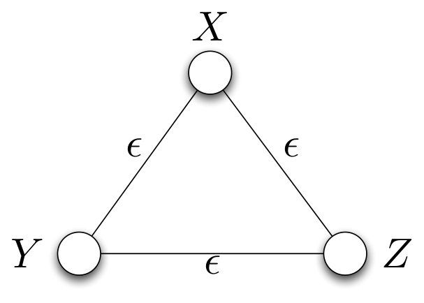
Refer to caption
(a) Source distribution
Refer to caption
(b) Target distribution
Fig. 8: Three random variable simulation example: Every pair of agents can achieve the desired simulation but the triple cannot.

Using the formula (47), we get

ρm​(X,Z,Y)\displaystyle\rho_{m}(X,Z;Y) =1−2​ϵ1−ϵ,\displaystyle=\frac{1-2\epsilon}{\sqrt{1-\epsilon}}\,, (48)
ρm​(U,W,V)\displaystyle\rho_{m}(U,W;V) =1−2​ϵ1−2​ϵ+2​ϵ2.\displaystyle=\frac{1-2\epsilon}{\sqrt{1-2\epsilon+2\epsilon^{2}}}\,. (49)

For 0<ϵ<12,0<\epsilon<\frac{1}{2}, we have 1−2​ϵ+2​ϵ2<1−ϵ,1-2\epsilon+2\epsilon^{2}<1-\epsilon, which gives ρm​(X,Z,Y)<ρm​(U,W,V).\rho_{m}(X,Z;Y)<\rho_{m}(U,W;V). This shows that even if agents Alice and Charlie were to combine their observations and their random variable generation tasks to form one agent Alice-Charlie, then Alice-Charlie and Bob cannot achieve the desired non-interactive simulation.

Example 5.

Consider the following choices of source distribution P⁡(x,y,z)P(x,y,z) and target distribution Q⁡(u,v,w).Q(u,v,w).

P⁡(x,y,z)={a0 if ​(x,y,z)=(0,0,0),a2 if ​(x,y,z)=(0,1,1),(1,0,1),(1,1,0),\displaystyle P(x,y,z)=\begin{cases}a_{0}&\mbox{ if }(x,y,z)=(0,0,0),\\ a_{2}&\mbox{ if }(x,y,z)=(0,1,1),(1,0,1),(1,1,0),\end{cases}

where

a0+3​a2=1,\displaystyle a_{0}+3a_{2}=1, (50)

i.e. (X,Y,Z)(X,Y,Z) take values on the 4 sequences that satisfy X⊕Y⊕Z=0X\oplus Y\oplus Z=0 (addition modulo 2).

Q⁡(u,v,w)={b0 if ​(u,v,w)=(0,0,0),b1 if ​(u,v,w)=(0,0,1),(0,1,0),(1,0,0),b2 if ​(u,v,w)=(0,1,1),(1,0,1),(1,1,0),b3 if ​(u,v,w)=(1,1,1).\displaystyle Q(u,v,w)=\begin{cases}b_{0}&\mbox{ if }(u,v,w)=(0,0,0),\\ b_{1}&\mbox{ if }(u,v,w)=(0,0,1),(0,1,0),(1,0,0),\\ b_{2}&\mbox{ if }(u,v,w)=(0,1,1),(1,0,1),(1,1,0),\\ b_{3}&\mbox{ if }(u,v,w)=(1,1,1).\end{cases}

We will choose these parameters so that for some 0<γ<1,0<\gamma<1, we have

b0+b1\displaystyle b_{0}+b_{1} =a0+2​a2​γ+a2​γ2,\displaystyle=a_{0}+2a_{2}\gamma+a_{2}\gamma^{2}, (51)
b1+b2\displaystyle b_{1}+b_{2} =a2​(1−γ2),\displaystyle=a_{2}(1-\gamma^{2}), (52)
b2+b3\displaystyle b_{2}+b_{3} =a2​(1−γ)2.\displaystyle=a_{2}(1-\gamma)^{2}~. (53)

Consider the question of whether (U,V,W)(U,V,W) can be simulated from (X,Y,Z).(X,Y,Z). For simulation of pair (U,V)(U,V) from (X,Y),(X,Y), note that if A1,A2∼Ber⁡(γ)A_{1},A_{2}\sim\Ber(\gamma) i.i.d. and mutually independent of (X,Y),(X,Y), then

(X⊕(A1⋅1X=1),Y⊕(A2⋅1Y=1))=d(U,V)\left(X\oplus(A_{1}\cdot 1_{X=1}),Y\oplus(A_{2}\cdot 1_{Y=1})\right)\stackrel{{\scriptstyle d}}{{=}}(U,V)

because of conditions (51), (52), (53). By symmetry then, every pair of agents can achieve the desired simulation.

Now, if we imagine two agents observe (X,Y)(X,Y) and ZZ respectively and are required to simulate (U,V)(U,V) and WW respectively, then again this is possible since (X,Y)(X,Y) uniquely determines Z,Z, so the agents now have access to shared randomness which can be used to generate any required joint distribution.

However, consider the specific choice:

a0=0.825,γ=0.2,b0=0.8,\displaystyle a_{0}=0.825,\gamma=0.2,b_{0}=0.8,

so that the other parameters are fixed from (50), (51), (52), (53) to be:

a2=0.058333​…,b1=0.0506666​…,b2=0.005333​…,b3=0.032.\displaystyle a_{2}=0.058333...,\qquad b_{1}=0.0506666...,\qquad b_{2}=0.005333...,\qquad b_{3}=0.032~.

Here, we find computationally that

κ\displaystyle\kappa :=inf{p≥1:(p,p,p)∈ℋ⁡(X,Y,Z)}=1.93​…;\displaystyle:=\inf\{p\geq 1:(p,p,p)\in\mathcal{H}(X;Y;Z)\}=1.93...; (54)
ζ\displaystyle\zeta :=inf{p≥1:(p,p,p)∈ℋ⁡(U,V,W)}=2.07​…..\displaystyle:=\inf\{p\geq 1:(p,p,p)\in\mathcal{H}(U;V;W)\}=2.07....~. (55)

We present numerical evidence supporting the above claims. Specifically, we will show that 1.85<κ<1.951.85<\kappa<1.95 and ζ>2.05.\zeta>2.05.

Using Hölder’s inequality, it is easy to verify that the following two statements are equivalent:

𝔼​f​(X)​g​(Y)​h​(Z)\displaystyle\mathbb{E}f(X)g(Y)h(Z) ≤‖f⁡(X)‖p​||g⁡(Y)||p|​|h⁡(Z)||p,∀f:𝒳→ℝ,g:𝒴→ℝ,h:𝒵→ℝ,\displaystyle\leq||f(X)||_{p}||g(Y)||_{p}||h(Z)||_{p},\ \forall f:\mathcal{X}\to\mathbb{R},g:\mathcal{Y}\to\mathbb{R},h:\mathcal{Z}\to\mathbb{R}, (56)
‖𝔼⁡[f⁡(X)​g​(Y)|Z]‖p′\displaystyle||\mathbb{E}[f(X)g(Y)|Z]||_{p^{\prime}} ≤‖f⁡(X)‖p||g⁡(Y)||p,∀f:𝒳→ℝ,g:𝒴→ℝ,\displaystyle\leq||f(X)||_{p}||g(Y)||_{p},\ \forall f:\mathcal{X}\to\mathbb{R},g:\mathcal{Y}\to\mathbb{R}, (57)

and furthermore, equivalently, all functions above may have co-domain ℝ≥0.\mathbb{R}_{\geq 0}. We choose f⁡(x)=(1+f)​1x=1+(1−f)​1x=0f(x)=(1+f)1_{x=1}+(1-f)1_{x=0} and g⁡(y)=(1+g)​1y=1+(1−g)​1y=0.g(y)=(1+g)1_{y=1}+(1-g)1_{y=0}. It suffices to consider functions of this form since the inequalities above are homogeneous. Fig. 9 shows contour plots of the ratio ‖𝔼⁡[f⁡(X)​g​(Y)|Z]‖p′‖f⁡(X)‖p||g⁡(Y)||p\frac{||\mathbb{E}[f(X)g(Y)|Z]||_{p^{\prime}}}{||f(X)||_{p}||g(Y)||_{p}} where the X-axis represents the variable f∈[−1,1]f\in[-1,1] and the Y-axis represents the variable g∈[−1,1].g\in[-1,1]. For p=1.95,p=1.95, the ratio is upper-bounded by 1, whereas for p=1.85,p=1.85, the ratio takes the value 1.0088​…1.0088... at f=g=−1.f=g=-1. (Note that the color bar in Fig. 9 has a maximum value of 1.01.0 for p=1.95p=1.95 and a maximum value of a little greater than 1.01.0 for p=1.85.p=1.85.) Thus, (1.95,1.95,1.95)∈ℋ⁡(X,Y,Z)(1.95,1.95,1.95)\in\mathcal{H}(X;Y;Z) but (1.85,1.85,1.85)∉ℋ⁡(X,Y,Z)(1.85,1.85,1.85)\not\in\mathcal{H}(X;Y;Z) and so, 1.85<κ<1.95.1.85<\kappa<1.95.

Refer to caption
(a) p=1.95p=1.95
Refer to caption
(b) p=1.85p=1.85
Fig. 9: Contour plots of the ratio ‖𝔼⁡[f⁡(X)​g​(Y)|Z]‖p′‖f⁡(X)‖p||g⁡(Y)||p\frac{||\mathbb{E}[f(X)g(Y)|Z]||_{p^{\prime}}}{||f(X)||_{p}||g(Y)||_{p}} where f⁡(x)=(1+f)​1x=1+(1−f)​1x=0f(x)=(1+f)1_{x=1}+(1-f)1_{x=0} and g⁡(y)=(1+g)​1y=1+(1−g)​1y=0.g(y)=(1+g)1_{y=1}+(1-g)1_{y=0}. The X-axis represents the variable f∈[−1,1]f\in[-1,1] and the Y-axis represents the variable g∈[−1,1].g\in[-1,1]. We see numerically that for p=1.95,p=1.95, the ratio is upper bounded by 11 everywhere, but for p=1.85,p=1.85, the ratio is maximized at f=g=−1f=g=-1 where it takes the value 1.0088​…1.0088... This implies that (1.95,1.95,1.95)∈ℋ⁡(X,Y,Z)(1.95,1.95,1.95)\in\mathcal{H}(X;Y;Z) but (1.85,1.85,1.85)∉ℋ⁡(X,Y,Z).(1.85,1.85,1.85)\not\in\mathcal{H}(X;Y;Z).

Now, consider the function δ⁡(θ)=9⋅1θ=1+1θ=0.\delta(\theta)=9\cdot 1_{\theta=1}+1_{\theta=0}. Then,

𝔼​δ​(U)​δ​(V)​δ​(W)\displaystyle\mathbb{E}\delta(U)\delta(V)\delta(W) =26.792\displaystyle=26.792 (58)
‖δ⁡(U)‖2.05​‖δ⁡(V)‖2.05||δ⁡(W)||2.05\displaystyle||\delta(U)||_{2.05}||\delta(V)||_{2.05}||\delta(W)||_{2.05} =(‖δ⁡(U)‖2.05)3=(2.9747​…)3=26.322​…<26.792.\displaystyle=\left(||\delta(U)||_{2.05}\right)^{3}=(2.9747...)^{3}=26.322...<26.792. (59)

This proves that (2.05,2.05,2.05)∉ℋ⁡(U,V,W)(2.05,2.05,2.05)\not\in\mathcal{H}(U;V;W) and so, ζ>2.05.\zeta>2.05.

Since κ<1.95\kappa<1.95 and ζ>2.05,\zeta>2.05, the inclusion ℋ⁡(X,Y,Z)⊆ℋ⁡(U,V,W)\mathcal{H}(X;Y;Z)\subseteq\mathcal{H}(U;V;W) is false and so, the simulation of (U,V,W)(U,V,W) from (X,Y,Z)(X,Y,Z) is impossible.

V Acknowledgements

We would like to thank Jingbo Liu, Elchanan Mossel and Vinod Prabhakaran for useful discussions.

Research support from the ARO MURI grant W911NF-08-1-0233, “Tools for the Analysis and Design of Complex Multi-Scale Network”, from the NSF grant CNS-0910702 and ECCS-1343398, from the NSF Science and Technology Center grant CCF-0939370,“Science of Information”, from Marvell Semiconductor Inc., and from the U.C. Discovery program is gratefully acknowledged.

References

  • [1] Amazon Prime Air, http://www.amazon.com/b?node=8037720011.
  • [2] Integration Innovation Inc., http://www.i3-corps.com/environmental.
  • [3] P. Gács and J. Körner, “Common information is far less than mutual information”, Problems of Control and Information Theory, vol. 2, no. 2, pp. 119–162, 1972.
  • [4] A.D. Wyner, “The common information of two dependent random variables”, IEEE Transactions on Information Theory, vol. 21, no. 2, pp. 163–179, March 1975.
  • [5] T.S. Han and S. Verdú, “Approximation theory of output statistics”, IEEE Transactions on Information Theory, vol. 39, no. 3, pp. 752–772, May 1993.
  • [6] P. Cuff, “Distributed channel synthesis”, IEEE Transactions on Information Theory, vol. 59, no. 11, pp. 7071–7096, November 2013.
  • [7] G. Kumar, C.T. Li, and A. El Gamal, “Exact common information”, in Proc. of IEEE ISIT, Honolulu, Hawaii, July 2014.
  • [8] P. Cuff, “Communication requirements for generating correlated random variables”, in Proc. of IEEE ISIT, Toronto, Canada, July 2008.
  • [9] P. Cuff, H. Permuter, and T. Cover, “Coordination capacity”, IEEE Transactions on Information Theory, vol. 56, no. 9, pp. 4181–4206, September 2010.
  • [10] A.A. Gohari and V. Anantharam, “Generating dependent random variables over networks”, in Proceedings of the IEEE Information Theory Workshop, Paraty, Brazil, October 2011, pp. 698–702.
  • [11] M.H. Yassaee, A.A. Gohari, and M.R. Aref, “Channel simulation via interactive communications”, in Proc. of IEEE ISIT, Cambridge, MA, July 2012.
  • [12] V. Anantharam and V. Borkar, “Common randomness and distributed control: A counterexample”, Systems and Control Letters, vol. 56, no. 7-8, pp. 568–572, July 2007.
  • [13] E. Mossel, R. O’Donnell, O. Regev, J. Steif, and B. Sudakov, “Non-interactive correlation distillation, inhomogeneous Markov chains, and the reverse Bonami-Beckner inequality”, Israel Journal of Mathematics, , no. 154, pp. 299–336, 2006.
  • [14] A. Bogdanov and E. Mossel, “On extracting common random bits from correlated sources”, IEEE Transactions on Information Theory, vol. 57, no. 10, pp. 6351 – 6355, October 2011.
  • [15] H.S. Witsenhausen, “On sequences of pairs of dependent random variables”, SIAM Journal on Applied Mathematics, vol. 28, no. 1, pp. 100–113, January 1975.
  • [16] Aline Bonami, “Ensembles Λ⁡(p)\Lambda(p) dans le dual de D∞D^{\infty}”, Ann. Inst. Fourier, vol. 18, no. 2, pp. 193–204, 1968.
  • [17] Aline Bonami, “Étude des coefficients de Fourier des fonctions de Lp​(G)L^{p}(G)”, Ann. Inst. Fourier (Grenoble), vol. 20, no. 2, pp. 335–402, 1970.
  • [18] Edward Nelson, “Construction of quantum fields from Markoff fields”, J. Functional Analysis, vol. 12, pp. 97–112, 1973.
  • [19] L. Gross, “Logarithmic Sobolev inequalities”, Amer. J. Math., vol. 97, pp. 1061–1083, 1975.
  • [20] William Beckner, “Inequalities in fourier analysis”, Ann. of Math., vol. 102, no. 1, pp. 159–182, 1975.
  • [21] Christer Borell, “Positivity improving operators and hypercontractivity”, Math. Z., vol. 180, no. 2, pp. 225–234, 1982.
  • [22] E. Mossel, K. Oleszkiewicz, and A. Sen, “On reverse hypercontractivity”, Geometric and Functional Analysis, vol. 23, no. 3, pp. 1062–1097, 2011.
  • [23] J. Kahn, G. Kalai, and N. Linial, “The influence of variables on Boolean functions”, in Proc. of 29th Annual Symposium on Foundations of Computer Science, 1988.
  • [24] E. Friedgut, “Boolean functions with low average sensitivity”, Combinatorica, vol. 18, pp. 27–36, 1998.
  • [25] E. Mossel, R. O’Donnell, and K. Oleszkiewicz, “Noise stability of functions with low influences: Invariance and Optimality”, in Proceedings of the 46th Annual Symposium on Foundations of Computer Science, 2005.
  • [26] E. Mossel and M. Racz, “A quantitative Gibbard-Satterthwaite theorem without neutrality”, in Proc. of the 44th Annual Symposium on Theory of Computing, 2012.
  • [27] R. Ahlswede and P. Gács, “Spreading of sets in product spaces and hypercontraction of the Markov operator”, Annals of Probability, vol. 4, pp. 925–939, 1976.
  • [28] M. Raginsky, “Logarithmic Sobolev inequalities and strong data processing theorems for discrete channels”, in Proc. of IEEE ISIT, Istanbul, Turkey, 2013.
  • [29] Yury Polyanskiy, “Hypothesis testing via a comparator and hypercontractivity”, On webpage, 2013, http://people.lids.mit.edu/yp/homepage/data/htstruct_journal.pdf.
  • [30] Y. Polyanskiy, “Hypercontractivity of spherical averages in Hamming space”, preprint at arxiv: 1309.3014, 2013.
  • [31] V. Anantharam, A. Gohari, S. Kamath, and C. Nair, “On hypercontractivity and a data processing inequality”, in Proc. of IEEE ISIT, Honolulu, Hawaii, July 2014.
  • [32] V. Anantharam, A. Gohari, S. Kamath, and C. Nair, “On hypercontractivity and the mutual information between Boolean functions”, in Proc. of the 51st Annual Allerton Conference on Communications, Control and Computing, Monticello, Illinois, October 2013.
  • [33] A. Rényi, “On measures of dependence”, Acta. Math. Acad. Sci. Hung., vol. 10, pp. 441–451, 1959.
  • [34] G.H. Hardy, J.E. Littlewood, and G. Pólya, Inequalities (2nd ed.), Cambridge University Press, Cambridge, 1952.
  • [35] G. Kumar and T. Courtade, “Which Boolean functions are most informative?”, in Proc. of IEEE ISIT, Istanbul, Turkey, 2013.
  • [36] Gowtham Kumar, “On sequences of pairs of dependent random variables: A simpler proof of the main result using SVD”, On webpage, July 2010, http://www.stanford.edu/~gowthamr/research/Witsenhausen_simpleproof.pdf.
  • [37] P. Billingsley, Probability and Measure (3rd ed.), Wiley, New York, 1995.

-A Proof of the claimed properties of ρm\rho_{m}

In this subsection, we prove the claimed properties of maximal correlation.

  • •

    (data processing inequality) For any functions ϕ,ψ,\phi,\psi, ρm​(X,Y)≥ρm​(ϕ⁡(X),ψ⁡(Y)).\rho_{m}(X;Y)\geq\rho_{m}(\phi(X),\psi(Y)).

    Proof: This is straightforward from the definition of ρm.\rho_{m}.

  • •

    (tensorization) If (X1,Y1)(X_{1},Y_{1}) and (X2,Y2)(X_{2},Y_{2}) are independent, then ρm​(X1,X2,Y1,Y2)=max⁡{ρm​(X1,Y1),ρm​(X2,Y2)}.\rho_{m}(X_{1},X_{2};Y_{1},Y_{2})=\max\{\rho_{m}(X_{1};Y_{1}),\rho_{m}(X_{2};Y_{2})\}.

    Proof: This property was shown by Witsenhausen [15]. The following exposition of Witsenhausen’s proof is by Kumar [36]. If we define |𝒳|×|𝒴||\mathcal{X}|\times|\mathcal{Y}| matrices P,QP,Q by Px,y=P⁡(x,y)P_{x,y}=P(x,y) and Qx,y=P⁡(x,y)P⁡(x)​P​(y),Q_{x,y}=\frac{P(x,y)}{\sqrt{P(x)P(y)}}, then the top two singular values of QQ are σ1​(Q)=1\sigma_{1}(Q)=1 and σ2​(Q)=ρm​(X,Y)\sigma_{2}(Q)=\rho_{m}(X;Y) (for proof, see [36]). The tensorization property then follows from the fact that the singular values of the tensor product of two matrices A⊗BA\otimes B are given by σi​(A)​σj​(B).\sigma_{i}(A)\sigma_{j}(B).

  • •

    (Lower semi-continuity) If the space of probability distributions on 𝒳×𝒴\mathcal{X}\times\mathcal{Y} is endowed with the total variation distance metric, then ρm​(X,Y)\rho_{m}(X;Y) is a lower semi-continuous function of the joint distribution P⁡(x,y).P(x,y).

    Proof: Suppose (X,Y),(X1,Y1),(X2,Y2),…(X,Y),(X_{1},Y_{1}),(X_{2},Y_{2}),\ldots are random variable pairs taking values in the finite set 𝒳×𝒴\mathcal{X}\times\mathcal{Y} satisfying dTV​((Xn,Yn),(X,Y))→0d_{\mathrm{TV}}((X_{n},Y_{n});(X,Y))\to 0 as n→∞.n\to\infty. We will show that ρ:=lim infn→∞ρm​(Xn,Yn)≥ρm​(X,Y).\rho:=\liminf_{n\to\infty}\rho_{m}(X_{n};Y_{n})\geq\rho_{m}(X;Y). Let {jn}n=1∞\{j_{n}\}_{n=1}^{\infty} be a subsequence so that ρ=limn→∞ρm​(Xjn,Yjn).\rho=\lim_{n\to\infty}\rho_{m}(X_{j_{n}};Y_{j_{n}}).

    For any ϵ>0,\epsilon>0, there exists a j⁡(ϵ)j(\epsilon) such that ρm​(Xjn,Yjn)≤ρ+ϵ\rho_{m}(X_{j_{n}};Y_{j_{n}})\leq\rho+\epsilon for all jn≥j⁡(ϵ).j_{n}\geq j(\epsilon). Fix any functions f:𝒳↦ℝ,g:𝒴↦ℝf:\mathcal{X}\mapsto\mathbb{R},g:\mathcal{Y}\mapsto\mathbb{R} such that 𝔼​f​(X)=𝔼​g​(Y)=0\mathbb{E}f(X)=\mathbb{E}g(Y)=0 and 𝔼​f​(X)2,𝔼​g​(Y)2≤1.\mathbb{E}f(X)^{2},\mathbb{E}g(Y)^{2}\leq 1. We will show 𝔼​f​(X)​g​(Y)≤ρ\mathbb{E}f(X)g(Y)\leq\rho which will complete the proof.

    If 𝔼​f​(X)2=0\mathbb{E}f(X)^{2}=0 or 𝔼​g​(Y)2=0,\mathbb{E}g(Y)^{2}=0, there is nothing to prove. So, suppose 𝔼​f​(X)2,𝔼​g​(Y)2>0.\mathbb{E}f(X)^{2},\mathbb{E}g(Y)^{2}>0. Since 𝒳×𝒴\mathcal{X}\times\mathcal{Y} is a finite set, dTV​((Xjn,Yjn),(X,Y))→0d_{\mathrm{TV}}((X_{j_{n}},Y_{j_{n}});(X,Y))\to 0 implies that Var⁡(f⁡(Xjn))→Var⁡(f⁡(X))>0,Var⁡(g⁡(Yjn))→Var⁡(g⁡(Y))>0.\Var(f(X_{j_{n}}))\to\Var(f(X))>0,\Var(g(Y_{j_{n}}))\to\Var(g(Y))>0. There exists j⁡(f,g)j(f,g) such that Var⁡(f⁡(Xjn))≥Var⁡(f⁡(X))2,Var⁡(g⁡(Yjn))≥Var⁡(g⁡(Y))2\Var(f(X_{j_{n}}))\geq\frac{\Var(f(X))}{2},\Var(g(Y_{j_{n}}))\geq\frac{\Var(g(Y))}{2} for all j≥n⁡(f,g).j\geq n(f,g).

    Define for jn≥max⁡{j⁡(ϵ),j⁡(f,g)}j_{n}\geq\max\{j(\epsilon),j(f,g)\} the functions fjn:𝒳↦ℝ,gjn:𝒴↦ℝf_{j_{n}}:\mathcal{X}\mapsto\mathbb{R},g_{j_{n}}:\mathcal{Y}\mapsto\mathbb{R} given by

    fjn​(X)=f⁡(Xjn)−𝔼​f​(Xjn)Var⁡(f⁡(Xjn)),\displaystyle f_{j_{n}}(X)=\frac{f(X_{j_{n}})-\mathbb{E}f(X_{j_{n}})}{\sqrt{\Var(f(X_{j_{n}}))}}~, (60)
    gjn​(Y)=g⁡(Yjn)−𝔼​g​(Yjn)Var⁡(g⁡(Yjn)),\displaystyle g_{j_{n}}(Y)=\frac{g(Y_{j_{n}})-\mathbb{E}g(Y_{j_{n}})}{\sqrt{\Var(g(Y_{j_{n}}))}}~, (61)

    which is possible since for such jnj_{n} we have Var⁡(f⁡(Xjn)),Var⁡(g⁡(Yjn))>0.\Var(f(X_{j_{n}})),\Var(g(Y_{j_{n}}))>0.

    Again, we will have 𝔼​fjn​(X)​gjn​(Y)→𝔼​f​(X)​g​(Y)𝔼​f​(X)2​𝔼​g​(Y)2≥𝔼​f​(X)​g​(Y).\mathbb{E}f_{j_{n}}(X)g_{j_{n}}(Y)\to\frac{\mathbb{E}f(X)g(Y)}{\sqrt{\mathbb{E}f(X)^{2}\mathbb{E}g(Y)^{2}}}\geq\mathbb{E}f(X)g(Y). But by definition, we have for jn≥max⁡{j⁡(ϵ),j⁡(f,g)}j_{n}\geq\max\{j(\epsilon),j(f,g)\} that 𝔼​fjn​(X)​gjn​(Y)≤ρm​(Xjn,Yjn)≤ρ+ϵ.\mathbb{E}f_{j_{n}}(X)g_{j_{n}}(Y)\leq\rho_{m}(X_{j_{n}};Y_{j_{n}})\leq\rho+\epsilon. This gives 𝔼​f​(X)​g​(Y)≤ρ+ϵ.\mathbb{E}f(X)g(Y)\leq\rho+\epsilon. Since ϵ>0\epsilon>0 was arbitrary, we have 𝔼​f​(X)​g​(Y)≤ρ.\mathbb{E}f(X)g(Y)\leq\rho.

-B Proof of the claimed properties of sps_{p}

In this subsection, we prove the claimed properties of sps_{p} for p≠1.p\neq 1.

  • •

    (data processing inequality) For any functions ϕ,ψ,\phi,\psi, sp​(X,Y)≥sp​(ϕ⁡(X),ψ⁡(Y)).s_{p}(X;Y)\geq s_{p}(\phi(X);\psi(Y)).

    Proof: Let W=ϕ⁡(X),Z=ψ⁡(Y).W=\phi(X),Z=\psi(Y). Suppose for 1≤q≤p,1\leq q\leq p, we have ‖𝔼⁡[g⁡(Y)|X]‖p≤||g⁡(Y)||q||\mathbb{E}[g(Y)|X]||_{p}\leq||g(Y)||_{q} for all functions g:𝒳↦ℝ.g:\mathcal{X}\mapsto\mathbb{R}. For any function of Z,Z, say θ⁡(Z),\theta(Z), we have

    ‖𝔼⁡[θ⁡(Z)|W]‖p\displaystyle||\mathbb{E}[\theta(Z)|W]||_{p} =||𝔼⁡[θ⁡(ψ⁡(Y))|ϕ⁡(X)]||p\displaystyle=||\mathbb{E}[\theta(\psi(Y))|\phi(X)]||_{p} (62)
    =(a)||𝔼⁡[𝔼⁡[θ⁡(ψ⁡(Y))|X]|ϕ⁡(X)]||p\displaystyle\stackrel{{\scriptstyle(a)}}{{=}}||\mathbb{E}[\mathbb{E}[\theta(\psi(Y))|X]|\phi(X)]||_{p} (63)
    ≤(b)||𝔼⁡[θ⁡(ψ⁡(Y))|X]||p\displaystyle\stackrel{{\scriptstyle(b)}}{{\leq}}||\mathbb{E}[\theta(\psi(Y))|X]||_{p} (64)
    ≤‖θ⁡(ψ⁡(Y))‖q\displaystyle\leq||\theta(\psi(Y))||_{q} (65)
    =‖θ⁡(Z)‖q,\displaystyle=||\theta(Z)||_{q}, (66)

    where (a) follows from successive conditioning and (b) follows from Jensen’s inequality: ‖𝔼⁡[A|ϕ⁡(X)]‖p≤||A||p.||\mathbb{E}[A|\phi(X)]||_{p}\leq||A||_{p}. Similarly, we can deal with the case 1≥q≥p.1\geq q\geq p. This completes the proof.

  • •

    (tensorization) If (X1,Y1)(X_{1},Y_{1}) and (X2,Y2)(X_{2},Y_{2}) are independent, then sp​(X1,X2,Y1,Y2)=max⁡{sp​(X1,Y1),sp​(X2,Y2)}.s_{p}(X_{1},X_{2};Y_{1},Y_{2})=\max\{s_{p}(X_{1};Y_{1}),s_{p}(X_{2};Y_{2})\}.

    Proof: Suppose (X1,Y1)∼P1​(x1,y1)(X_{1},Y_{1})\sim P_{1}(x_{1},y_{1}) and (X2,Y2)∼P2​(x2,y2)(X_{2},Y_{2})\sim P_{2}(x_{2},y_{2}) are both (p,q)(p,q)-hypercontractive, with p<1,p≠0.p<1,p\neq 0. We remark that for the case of p=0,p=0, we take limits in the standard way. Then,

    𝔼​f​(X1)​g​(Y1)\displaystyle\mathbb{E}f(X_{1})g(Y_{1}) ≥‖f⁡(X1)‖p′​‖g⁡(Y1)‖q​∀f:𝒳1↦ℝ>0,∀g:𝒴1↦ℝ>0;\displaystyle\geq||f(X_{1})||_{p^{\prime}}||g(Y_{1})||_{q}\ \forall\ f:\mathcal{X}_{1}\mapsto\mathbb{R}_{>0},\ \ \forall\ g:\mathcal{Y}_{1}\mapsto\mathbb{R}_{>0}; (67)
    𝔼​f​(X2)​g​(Y2)\displaystyle\mathbb{E}f(X_{2})g(Y_{2}) ≥‖f⁡(X2)‖p′​‖g⁡(Y2)‖q​∀f:𝒳2↦ℝ>0,∀g:𝒴2↦ℝ>0.\displaystyle\geq||f(X_{2})||_{p^{\prime}}||g(Y_{2})||_{q}\ \forall\ f:\mathcal{X}_{2}\mapsto\mathbb{R}_{>0},\ \ \forall\ g:\mathcal{Y}_{2}\mapsto\mathbb{R}_{>0}. (68)

    Now, fix any positive-valued functions f:𝒳1×𝒳2↦ℝ>0,g:𝒴1×𝒴2↦ℝ>0.f:\mathcal{X}_{1}\times\mathcal{X}_{2}\mapsto\mathbb{R}_{>0},g:\mathcal{Y}_{1}\times\mathcal{Y}_{2}\mapsto\mathbb{R}_{>0}.

    𝔼​f​(X1,X2)​g​(Y1,Y2)\displaystyle\mathbb{E}f(X_{1},X_{2})g(Y_{1},Y_{2}) =∑x1,y1P1​(x1,y1)​∑x2,y2P2​(x2,y2)​f​(x1,x2)​g​(y1,y2)\displaystyle=\sum_{x_{1},y_{1}}P_{1}(x_{1},y_{1})\sum_{x_{2},y_{2}}P_{2}(x_{2},y_{2})f(x_{1},x_{2})g(y_{1},y_{2}) (69)
    ≥(a)∑x1,y1P1​(x1,y1)​(∑x2PX2​(x2)​f​(x1,x2)p′)1p′​(∑y2PY2​(y2)​g​(y1,y2)q)1q\displaystyle\stackrel{{\scriptstyle(a)}}{{\geq}}\sum_{x_{1},y_{1}}P_{1}(x_{1},y_{1})\left(\sum_{x_{2}}P_{X_{2}}(x_{2})f(x_{1},x_{2})^{p^{\prime}}\right)^{\frac{1}{p^{\prime}}}\left(\sum_{y_{2}}P_{Y_{2}}(y_{2})g(y_{1},y_{2})^{q}\right)^{\frac{1}{q}} (70)
    ≥(b)(∑x1,x2PX1​(x1)​PX2​(x2)​f​(x1,x2)p′)1p′​(∑y1,y2PY1​(y1)​PY2​(y2)​g​(y1,y2)q)1q\displaystyle\stackrel{{\scriptstyle(b)}}{{\geq}}\left(\sum_{x_{1},x_{2}}P_{X_{1}}(x_{1})P_{X_{2}}(x_{2})f(x_{1},x_{2})^{p^{\prime}}\right)^{\frac{1}{p^{\prime}}}\left(\sum_{y_{1},y_{2}}P_{Y_{1}}(y_{1})P_{Y_{2}}(y_{2})g(y_{1},y_{2})^{q}\right)^{\frac{1}{q}} (71)
    =‖f⁡(X1,X2)‖p′||g⁡(Y1,Y2)||q,\displaystyle=||f(X_{1},X_{2})||_{p^{\prime}}||g(Y_{1},Y_{2})||_{q}, (72)

    where (a) follows from (68) and (b) follows from (67). This means ((X1,X2),(Y1,Y2))((X_{1},X_{2}),(Y_{1},Y_{2})) is (p,q)(p,q)-hypercontractive. It is easy to see that if one of (X1,Y1)(X_{1},Y_{1}) or (X2,Y2)(X_{2},Y_{2}) is not (p,q)(p,q)-hypercontractive, then ((X1,X2),(Y1,Y2))((X_{1},X_{2}),(Y_{1},Y_{2})) is not (p,q)(p,q)-hypercontractive. Thus,

    qp∗​(X1,X2,Y1,Y2)=min⁡{qp∗​(X1,Y1),qp∗​(X2,Y2)},q_{p}^{*}(X_{1},X_{2};Y_{1},Y_{2})=\min\{q_{p}^{*}(X_{1};Y_{1}),q_{p}^{*}(X_{2};Y_{2})\},

    which gives

    sp​(X1,X2,Y1,Y2)=max⁡{sp​(X1,Y1),sp​(X2,Y2)}.s_{p}(X_{1},X_{2};Y_{1},Y_{2})=\max\{s_{p}(X_{1};Y_{1}),s_{p}(X_{2};Y_{2})\}.

    For p>1,p>1, the proof is similar; in this case, we find

    qp∗​(X1,X2,Y1,Y2)=max⁡{qp∗​(X1,Y1),qp∗​(X2,Y2)},q_{p}^{*}(X_{1},X_{2};Y_{1},Y_{2})=\max\{q_{p}^{*}(X_{1};Y_{1}),q_{p}^{*}(X_{2};Y_{2})\},

    and

    sp​(X1,X2,Y1,Y2)=max⁡{sp​(X1,Y1),sp​(X2,Y2)}.s_{p}(X_{1},X_{2};Y_{1},Y_{2})=\max\{s_{p}(X_{1};Y_{1}),s_{p}(X_{2};Y_{2})\}.
  • •

    (lower semi-continuity) If the space of probability distributions on 𝒳×𝒴\mathcal{X}\times\mathcal{Y} is endowed with the total variation distance metric, then sp​(X,Y)s_{p}(X;Y) is a lower semi-continuous function of the joint distribution P⁡(x,y).P(x,y).

    Proof: Let us fix p<1.p<1. An identical proof holds for the case of p>1.p>1. Suppose (X,Y),(X1,Y1),(X2,Y2),…(X,Y),(X_{1},Y_{1}),(X_{2},Y_{2}),\ldots are random variable pairs taking values in the finite set 𝒳×𝒴\mathcal{X}\times\mathcal{Y} satisfying dTV​((Xn,Yn),(X,Y))→0d_{\mathrm{TV}}((X_{n},Y_{n});(X,Y))\to 0 as n→∞.n\to\infty. Let s:=lim infn→∞sp​(Xn,Yn)≥0.s:=\liminf_{n\to\infty}s_{p}(X_{n};Y_{n})\geq 0. We will show that s≥sp​(X,Y).s\geq s_{p}(X;Y). Let {jn}n=1∞\{j_{n}\}_{n=1}^{\infty} be a subsequence so that s=limn→∞sp​(Xjn,Yjn).s=\lim_{n\to\infty}s_{p}(X_{j_{n}};Y_{j_{n}}).

    We may assume without loss of generality that s<1.s<1. For any ϵ>0,\epsilon>0, there exists a j⁡(ϵ)j(\epsilon) such that sp​(Xjn,Yjn)≤s+ϵs_{p}(X_{j_{n}};Y_{j_{n}})\leq s+\epsilon for all jn≥j⁡(ϵ).j_{n}\geq j(\epsilon). We would like to show sp​(X,Y)≤s,s_{p}(X;Y)\leq s, i.e., that for any functions f:𝒳↦ℝ>0,g:𝒴↦ℝ>0,f:\mathcal{X}\mapsto\mathbb{R}_{>0},g:\mathcal{Y}\mapsto\mathbb{R}_{>0}, the following holds:

    𝔼​f​(X)​g​(Y)\displaystyle\mathbb{E}f(X)g(Y) ≥‖f⁡(X)‖p′||g⁡(Y)||1+s⁡(p−1).\displaystyle\geq||f(X)||_{p^{\prime}}||g(Y)||_{1+s(p-1)}. (73)

    For any given functions f:𝒳↦ℝ>0,g:𝒴↦ℝ>0,f:\mathcal{X}\mapsto\mathbb{R}_{>0},g:\mathcal{Y}\mapsto\mathbb{R}_{>0}, and any jn≥j⁡(ϵ),j_{n}\geq j(\epsilon), we have from sp​(Xjn,Yjn)≤s+ϵs_{p}(X_{j_{n}};Y_{j_{n}})\leq s+\epsilon that for jn≥n⁡(ϵ),j_{n}\geq n(\epsilon),

    𝔼​f​(Xjn)​g​(Yjn)\displaystyle\mathbb{E}f(X_{j_{n}})g(Y_{j_{n}}) ≥‖f⁡(Xjn)‖p′||g⁡(Yjn)||1+(s+ϵ)​(p−1).\displaystyle\geq||f(X_{j_{n}})||_{p^{\prime}}||g(Y_{j_{n}})||_{1+(s+\epsilon)(p-1)}. (74)

    From the portmanteau lemma [37], we get

    𝔼​f​(X)​g​(Y)\displaystyle\mathbb{E}f(X)g(Y) ≥‖f⁡(X)‖p′||g⁡(Y)||1+(s+ϵ)​(p−1).\displaystyle\geq||f(X)||_{p^{\prime}}||g(Y)||_{1+(s+\epsilon)(p-1)}. (75)

    Since this is true for each ϵ>0,\epsilon>0, we get from continuity of ||.||q||.||_{q} in qq that

    𝔼​f​(X)​g​(Y)\displaystyle\mathbb{E}f(X)g(Y) ≥‖f⁡(X)‖p′||g⁡(Y)||1+s⁡(p−1).\displaystyle\geq||f(X)||_{p^{\prime}}||g(Y)||_{1+s(p-1)}. (76)

    Since this is true for any functions f:𝒳↦ℝ>0,g:𝒴↦ℝ>0,f:\mathcal{X}\mapsto\mathbb{R}_{>0},g:\mathcal{Y}\mapsto\mathbb{R}_{>0}, we have sp​(X,Y)≤s.s_{p}(X;Y)\leq s.

    Remark 7.

    Note that this implies that qp​(X,Y)=1+sp​(X,Y)​(p−1)q_{p}(X;Y)=1+s_{p}(X;Y)(p-1) is lower semi-continuous in the joint distribution for fixed p>1p>1 and upper semi-continuous in the joint distribution for fixed p<1.p<1.

    Remark 8.

    Lower semi-continuity of ρm\rho_{m} and sps_{p} was enough for our purposes. Indeed, ρm\rho_{m} and sps_{p} are not continuous in the underlying joint distribution. As an example, let (Xn,Yn)(X_{n},Y_{n}) be binary-valued and have a joint probability distribution given by [1n001−1n].\begin{bmatrix}\frac{1}{n}&0\\ 0&1-\frac{1}{n}\end{bmatrix}. Then, (Xn,Yn)→d(X,Y)(X_{n},Y_{n})\stackrel{{\scriptstyle d}}{{\to}}(X,Y) where (X,Y)(X,Y) has a joint probability distribution given by [0001].\begin{bmatrix}0&0\\ 0&1\end{bmatrix}. But ρm​(Xn,Yn)=sp​(Xn,Yn)=1\rho_{m}(X_{n};Y_{n})=s_{p}(X_{n};Y_{n})=1 for each nn and each p≠1,p\neq 1, while ρm​(X,Y)=sp​(X,Y)=0.\rho_{m}(X;Y)=s_{p}(X;Y)=0.

    However, it may be shown that if (X,Y)∼P⁡(x,y)(X,Y)\sim P(x,y) satisfies the assumption P⁡(x)>0∀x∈𝒳,P⁡(y)>0∀y∈𝒴,P(x)>0\ \ \forall x\in\mathcal{X},P(y)>0\ \ \ \forall y\in\mathcal{Y}, then (Xn,Yn)→d(X,Y)(X_{n},Y_{n})\stackrel{{\scriptstyle d}}{{\to}}(X,Y) implies limn→∞ρm​(Xn,Yn)=ρm​(X,Y).\lim_{n\to\infty}\rho_{m}(X_{n};Y_{n})=\rho_{m}(X;Y). To see this, use the characterization ρm​(X,Y)=σ2​(AX;Y),\rho_{m}(X;Y)=\sigma_{2}(A_{X;Y}), where the matrix AX;YA_{X;Y} is specified by [AX;Y]x,y=P⁡(x,y)P⁡(x)​P​(y)[A_{X;Y}]_{x,y}=\frac{P(x,y)}{\sqrt{P(x)P(y)}} and σ2​(⋅)\sigma_{2}(\cdot) is the second largest singular value [15, 36]. Under the assumption, AXn;Yn→AX;YA_{X_{n};Y_{n}}\to A_{X;Y} and the second largest singular value is a continuous matrix functional.

-C Limiting properties of sps_{p}: Proofs of Thm. 2 and Corollary 2

As in [22], we define for any non-negative random variable X,X, the function Ent⁡(X):=𝔼⁡[X​log⁡X]−𝔼⁡[X]⋅log⁡𝔼⁡[X],\Ent(X):=\mathbb{E}[X\log X]-\mathbb{E}[X]\cdot\log\mathbb{E}[X], where by convention 0​log⁡0:=0.0\log 0:=0. By strict convexity of the function x↦x​log⁡xx\mapsto x\log x and Jensen’s inequality, we get that Ent⁡(X)≥0\Ent(X)\geq 0 and equality holds if and only if XX is a constant almost surely. Also, we note that Ent⁡(⋅)\Ent(\cdot) is homogenous, that is, Ent⁡(a​X)=a​Ent⁡(X)\Ent(aX)=a\Ent(X) for any a≥0.a\geq 0.

We begin by presenting first a simple lemma.

Lemma 1.

For any random variable ZZ satisfying 0≤Z≤K0\leq Z\leq K for some constant K>0K>0 and 𝔼​Z=1\mathbb{E}Z=1 and 0≤u≤1,0\leq u\leq 1, we have

1+u​Ent⁡(Z)−u2​L1​(K)≤‖Z‖1+u≤1+u​Ent⁡(Z)+u2​L0​(K),\displaystyle 1+u\Ent(Z)-u^{2}L_{1}(K)\leq\|Z\|_{1+u}\leq 1+u\Ent(Z)+u^{2}L_{0}(K), (77)

where L0​(K)=12​max⁡{Ku,1}​max0≤z≤K​z​(log⁡z)2L_{0}(K)=\frac{1}{2}\max\{K^{u},1\}\max_{0\leq z\leq K}z(\log z)^{2} and L1​(K)=(max0≤z≤K⁡|z​log⁡z|)+12​(max0≤z≤K⁡|z​log⁡z|)2.L_{1}(K)=(\max_{0\leq z\leq K}|z\log z|)+\frac{1}{2}(\max_{0\leq z\leq K}|z\log z|)^{2}.

Proof of Lemma 1.

For any constant 0≤u≤10\leq u\leq 1 and any θ∈ℝ,\theta\in\mathbb{R}, a Taylor’s series expansion yields

1+u​θ≤eu​θ≤1+u​θ+u22​θ2​max⁡{eu​θ,1}.1+u\theta\leq e^{u\theta}\leq 1+u\theta+\frac{u^{2}}{2}\theta^{2}\max\{e^{u\theta},1\}~.

Thus, for any 0≤z≤K0\leq z\leq K for some constant K>0,K>0, and 0≤u≤1,0\leq u\leq 1, we have using z1+u=z​eu​log⁡z,z^{1+u}=ze^{u\log z},

z+u​z​log⁡z≤z1+u≤z+u​z​log​z+u22​z​(log⁡z)2​max​{zu,1}.z+uz\log z\leq z^{1+u}\leq z+uz\log z+\frac{u^{2}}{2}z(\log z)^{2}\max\{z^{u},1\}~.

For any random variable ZZ satisfying 0≤Z≤K0\leq Z\leq K almost surely and any 0≤u≤1,0\leq u\leq 1,

𝔼​Z+u​𝔼​[Z​log⁡Z]≤𝔼⁡[Z1+u]\displaystyle\mathbb{E}Z+u\mathbb{E}[Z\log Z]\leq\mathbb{E}[Z^{1+u}] ≤𝔼​Z+u​𝔼​[Z​log⁡Z]+u22​max⁡{Ku,1}​𝔼​[Z​(log⁡Z)2]\displaystyle\leq\mathbb{E}Z+u\mathbb{E}[Z\log Z]+\frac{u^{2}}{2}\max\{K^{u},1\}\mathbb{E}[Z(\log Z)^{2}]
≤𝔼​Z+u​𝔼​[Z​log⁡Z]+u2​L0​(K).\displaystyle\leq\mathbb{E}Z+u\mathbb{E}[Z\log Z]+u^{2}L_{0}(K)~. (78)

Now, again a Taylor’s expansion yields that for 0≤r≤10\leq r\leq 1 and any x≥0,x\geq 0, we have

1+r​x−x22​r​(1−r)≤(1+x)r≤1+r​x.\displaystyle 1+rx-\frac{x^{2}}{2}r(1-r)\leq(1+x)^{r}\leq 1+rx~. (79)

Suppose ZZ is any random variable that satisfies 0≤Z≤K0\leq Z\leq K and 𝔼​Z=1.\mathbb{E}Z=1. Then 𝔼⁡[Z​log⁡Z]=Ent⁡(Z)≥0.\mathbb{E}[Z\log Z]=\Ent(Z)\geq 0. For any 0≤u≤1,0\leq u\leq 1, we get using the lower bounds in both (78) and (79) with the choice r=11+ur=\frac{1}{1+u} and x=u​Ent⁡(Z),x=u\Ent(Z),

1+11+u​u​Ent⁡(Z)−u2​Ent⁡(Z)22​11+u​u1+u≤(𝔼⁡[Z1+u])11+u.\displaystyle 1+\frac{1}{1+u}u\Ent(Z)-\frac{u^{2}\Ent(Z)^{2}}{2}\frac{1}{1+u}\frac{u}{1+u}\leq\left(\mathbb{E}[Z^{1+u}]\right)^{\frac{1}{1+u}}.

Similarly, using the upper bounds in both (78) and (79) with the choice r=11+ur=\frac{1}{1+u} and x=u​Ent⁡(Z)+u2​L0​(K),x=u\Ent(Z)+u^{2}L_{0}(K), we get

(𝔼⁡[Z1+u])11+u≤1+11+u​u​Ent⁡(Z)+11+u​u2​L0​(K).\displaystyle\left(\mathbb{E}[Z^{1+u}]\right)^{\frac{1}{1+u}}\leq 1+\frac{1}{1+u}u\Ent(Z)+\frac{1}{1+u}u^{2}L_{0}(K)~.

Putting the above two inequalities together,

1+11+u​u​Ent⁡(Z)−u2​Ent⁡(Z)22​11+u​u1+u≤‖Z‖1+u≤1+11+u​u​Ent⁡(Z)+11+u​u2​L0​(K).\displaystyle 1+\frac{1}{1+u}u\Ent(Z)-\frac{u^{2}\Ent(Z)^{2}}{2}\frac{1}{1+u}\frac{u}{1+u}\leq\|Z\|_{1+u}\leq 1+\frac{1}{1+u}u\Ent(Z)+\frac{1}{1+u}u^{2}L_{0}(K).

Define L2​(K)=max0≤z≤K⁡|z​log⁡z|L_{2}(K)=\max_{0\leq z\leq K}|z\log z| and observing that for 0≤u≤1,0\leq u\leq 1, we have 12≤11+u≤1,\frac{1}{2}\leq\frac{1}{1+u}\leq 1, we obtain

1+u​Ent⁡(Z)1+u−u32​L2​(K)2≤‖Z‖1+u≤1+u​Ent⁡(Z)1+u+u2​L0​(K).\displaystyle 1+\frac{u\Ent(Z)}{1+u}-\frac{u^{3}}{2}L_{2}(K)^{2}\leq\|Z\|_{1+u}\leq 1+\frac{u\Ent(Z)}{1+u}+u^{2}L_{0}(K).

Further using the fact that for 0≤u≤1,0\leq u\leq 1, we have 1−u≤11+u≤1,1-u\leq\frac{1}{1+u}\leq 1, we get

1+u​Ent⁡(Z)−u2​L2​(K)−u32​L2​(K)2≤‖Z‖1+u≤1+u​Ent⁡(Z)+u2​L0​(K).\displaystyle 1+u\Ent(Z)-u^{2}L_{2}(K)-\frac{u^{3}}{2}L_{2}(K)^{2}\leq\|Z\|_{1+u}\leq 1+u\Ent(Z)+u^{2}L_{0}(K).

Finally, since L1​(K)=L2​(K)+12​L2​(K)2L_{1}(K)=L_{2}(K)+\frac{1}{2}L_{2}(K)^{2} and u≤1,u\leq 1, we have

1+u​Ent⁡(Z)−u2​L1​(K)≤‖Z‖1+u≤1+u​Ent⁡(Z)+u2​L0​(K).\displaystyle 1+u\Ent(Z)-u^{2}L_{1}(K)\leq\|Z\|_{1+u}\leq 1+u\Ent(Z)+u^{2}L_{0}(K). (80)

∎

Next, we present the proof of Thm. 2.

Proof of Theorem 2 .

The theorem is easily seen to be true when YY is a constant almost surely. We assume then that this is not the case and that PY​(y)>0P_{Y}(y)>0 for all y∈𝒴y\in\mathcal{Y} and PX​(x)>0P_{X}(x)>0 for all x∈𝒳x\in\mathcal{X} without loss of generality. Define s:=supEnt⁡(𝔼⁡[g⁡(Y)|X])Ent⁡(g⁡(Y)),s:=\sup\frac{\Ent(\mathbb{E}[g(Y)|X])}{\Ent(g(Y))}, where the supremum is taken over functions g:𝒴↦ℝ≥0g:\mathcal{Y}\mapsto\mathbb{R}_{\geq 0} such that g⁡(Y)g(Y) is not a constant almost surely.

For any distribution RY​(y)≢PY​(y)R_{Y}(y)\not\equiv P_{Y}(y) consider the non-constant non-negative valued function gg given by g⁡(y):=RY​(y)PY​(y).g(y):=\frac{R_{Y}(y)}{P_{Y}(y)}. This choice yields Ent(g(Y))=D(RY(y)||PY(y))\Ent(g(Y))=D(R_{Y}(y)||P_{Y}(y)) and Ent(𝔼[g(Y)|X])=D(RX(x)||PX(x))),\Ent(\mathbb{E}[g(Y)|X])=D(R_{X}(x)||P_{X}(x))), where RX​(x)=∑yPX,Y​(x,y)PY​(y)​RY​(y).R_{X}(x)=\sum_{y}\frac{P_{X,Y}(x,y)}{P_{Y}(y)}R_{Y}(y). Along with homogeneity of Ent⁡(⋅),\Ent(\cdot), this means that s=s∗​(Y,X)s=s^{*}(Y;X) and thus, from the data processing inequality 0≤s≤1.0\leq s\leq 1.

For non-negative g,g, we always have

‖𝔼⁡[g⁡(Y)|X]‖1=‖g⁡(Y)‖1∀g:𝒴↦ℝ≥0.||\mathbb{E}[g(Y)|X]||_{1}=||g(Y)||_{1}\ \ \forall g:\mathcal{Y}\mapsto\mathbb{R}_{\geq 0}. (81)

Let 𝒢\mathcal{G} be the set of all non-negative functions g:𝒴↦ℝ≥0g:\mathcal{Y}\mapsto\mathbb{R}_{\geq 0} that satisfy ‖g⁡(Y)‖1=1.||g(Y)||_{1}=1. Note that for any g∈𝒢,g\in\mathcal{G}, both g⁡(Y)g(Y) and 𝔼⁡[g⁡(Y)|X]\mathbb{E}[g(Y)|X] are bounded between 00 and K:=1miny⁡PY​(y)K:=\frac{1}{\min_{y}P_{Y}(y)} almost surely.

If 0≤m≤10\leq m\leq 1 is any parameter satisfying m<s,m<s, then (1+τ,1+m​τ)∉ℛ⁡(X,Y)(1+\tau,1+m\tau)\not\in\mathcal{R}(X;Y) for all sufficiently small τ>0.\tau>0. To see this, fix g0g_{0} to be any function in 𝒢\mathcal{G} that satisfies

Ent⁡(𝔼⁡[g0​(Y)|X])Ent⁡(g0​(Y))≥m+δ2,\frac{\Ent(\mathbb{E}[g_{0}(Y)|X])}{\Ent(g_{0}(Y))}\geq m+\frac{\delta}{2}, (82)

where δ:=s−m.\delta:=s-m. From Lemma 1, we have that for any g∈𝒢,g\in\mathcal{G},

1+m​τ​Ent⁡(g⁡(Y))−m2​τ2​L1​(K)≤‖g⁡(Y)‖1+m​τ≤1+m​τ​Ent⁡(g⁡(Y))+m2​τ2​L0​(K),\displaystyle 1+m\tau\Ent(g(Y))-m^{2}\tau^{2}L_{1}(K)\leq||g(Y)||_{1+m\tau}\leq 1+m\tau\Ent(g(Y))+m^{2}\tau^{2}L_{0}(K), (83)
1+τ​Ent⁡(𝔼⁡[g⁡(Y)|X])−τ2​L1​(K)≤‖𝔼⁡[g⁡(Y)|X]‖1+τ≤1+τ​Ent⁡(𝔼⁡[g⁡(Y)|X])+τ2​L0​(K).\displaystyle 1+\tau\Ent(\mathbb{E}[g(Y)|X])-\tau^{2}L_{1}(K)\leq||\mathbb{E}[g(Y)|X]||_{1+\tau}\leq 1+\tau\Ent(\mathbb{E}[g(Y)|X])+\tau^{2}L_{0}(K). (84)

Putting together (82), (83), (84), we get the existence of τ0>0\tau_{0}>0 such that

‖𝔼⁡[g0​(Y)|X]‖1+τ>‖g0​(Y)‖1+m​τ∀τ:0<τ≤τ0.||\mathbb{E}[g_{0}(Y)|X]||_{1+\tau}>||g_{0}(Y)||_{1+m\tau}\ \ \forall\tau:0<\tau\leq\tau_{0}. (85)

Thus, s=s∗​(Y,X)≥lim supp→1+sp​(X,Y)=lim supp→1+qp∗​(X,Y)−1p−1.s=s^{*}(Y;X)\geq\limsup_{p\to 1^{+}}s_{p}(X;Y)=\limsup_{p\to 1^{+}}\frac{q_{p}^{*}(X;Y)-1}{p-1}.

If for some 0≤m≤10\leq m\leq 1 we have m>s,m>s, then define for any g∈𝒢,g\in\mathcal{G},

τ(g):=max{ζ:0≤ζ≤1,||𝔼[g(Y)|X]||1+η≤||g(Y)||1+m​η for all 0≤η≤ζ}.\tau(g):=\max\{\zeta:0\leq\zeta\leq 1,||\mathbb{E}[g(Y)|X]||_{1+\eta}\leq||g(Y)||_{1+m\eta}\mbox{ for all }0\leq\eta\leq\zeta\}.

From (81), we have τ⁡(g)≥0\tau(g)\geq 0 for all g∈𝒢.g\in\mathcal{G}.

Let g1∈𝒢g_{1}\in\mathcal{G} denote the constant function 1. Then, τ⁡(g1)=1.\tau(g_{1})=1. Lemma 2 below shows that there is an open neighborhood UU of g1g_{1} in 𝒢\mathcal{G} and a constant τ0>0\tau_{0}>0 such that τ⁡(g)≥τ0​∀g∈U.\tau(g)\geq\tau_{0}\ \forall g\in U.

Over the compact set 𝒢∖U,\mathcal{G}\setminus U, we define

τ′(g):=max{ζ:0≤ζ≤1,1+ηEnt(𝔼[g(Y)|X])+η2L0(K)≤1+mηEnt(g(Y))−m2η2L1(K) for all 0≤η≤ζ}.\tau^{\prime}(g):=\max\{\zeta:0\leq\zeta\leq 1,1+\eta\Ent(\mathbb{E}[g(Y)|X])+\eta^{2}L_{0}(K)\leq 1+m\eta\Ent(g(Y))-m^{2}\eta^{2}L_{1}(K)\mbox{ for all }0\leq\eta\leq\zeta\}.

Then, τ′​(g)≤τ⁡(g)\tau^{\prime}(g)\leq\tau(g) from Lemma 1. And indeed,

τ′​(g)=min⁡{m​Ent⁡(g⁡(Y))−Ent⁡(𝔼⁡[g⁡(Y)|X])L0​(K)+m2​L1​(K),1}.\tau^{\prime}(g)=\min\left\{\frac{m\Ent(g(Y))-\Ent(\mathbb{E}[g(Y)|X])}{L_{0}(K)+m^{2}L_{1}(K)},1\right\}.

Since τ′​(g)\tau^{\prime}(g) is continuous in gg over 𝒢∖U,\mathcal{G}\setminus U, and furthermore strictly positive over that set (since m>sm>s and because Ent⁡(g⁡(Y))>0\Ent(g(Y))>0 for gg non-constant), we have that τ′\tau^{\prime} attains its infimum over the compact set 𝒢∖U.\mathcal{G}\setminus U. Since τ′​(g)≤τ⁡(g),\tau^{\prime}(g)\leq\tau(g), we also have that infg∈𝒢∖Uτ⁡(g)>0.\inf_{g\in\mathcal{G}\setminus U}\tau(g)>0.

Then, infg∈𝒢τ⁡(g)=min⁡{τ0,infg∈𝒢∖Uτ⁡(g)}>0.\inf_{g\in\mathcal{G}}\tau(g)=\min\left\{\tau_{0},\inf_{g\in\mathcal{G}\setminus U}\tau(g)\right\}>0. Using homogeneity of the norm, this establishes that (1+τ,1+m​τ)∈ℛ⁡(X,Y)(1+\tau,1+m\tau)\in\mathcal{R}(X;Y) for all 0≤τ≤τ00\leq\tau\leq\tau_{0} for some τ0>0\tau_{0}>0 and thus, that s=s∗​(Y,X)≤lim infp→1+sp​(X,Y)=lim infp→1+qp∗​(X,Y)−1p−1.s=s^{*}(Y;X)\leq\liminf_{p\to 1^{+}}s_{p}(X;Y)=\liminf_{p\to 1^{+}}\frac{q_{p}^{*}(X;Y)-1}{p-1}.

Therefore, s=s∗​(Y,X)=limp→1+sp​(X,Y)=limp→1+qp∗​(X,Y)−1p−1.s=s^{*}(Y;X)=\lim_{p\to 1^{+}}s_{p}(X;Y)=\lim_{p\to 1^{+}}\frac{q_{p}^{*}(X;Y)-1}{p-1}.

Similarly, we can show the reverse hypercontractive case namely, that s=s∗​(Y,X)=limp→1−sp​(X,Y)=limp→1−qp∗​(X,Y)−1p−1.s=s^{*}(Y;X)=\lim_{p\to 1^{-}}s_{p}(X;Y)=\lim_{p\to 1^{-}}\frac{q_{p}^{*}(X;Y)-1}{p-1}. This completes the proof of the theorem.

Lemma 2.

When 1≥m>s,1\geq m>s, there exists an open neighborhood UU of the constant function g1g_{1} in 𝒢\mathcal{G} and a constant τ0>0\tau_{0}>0 such that τ⁡(g)≥τ0\tau(g)\geq\tau_{0} for all g∈U.g\in U.

Proof of Lemma 2.

Let ℱ\mathcal{F} denote the set of all functions f:𝒴↦ℝf:\mathcal{Y}\mapsto\mathbb{R} such that 𝔼⁡[f⁡(Y)]=0\mathbb{E}[f(Y)]=0 and 𝔼⁡[f​(Y)2]=1.\mathbb{E}[f(Y)^{2}]=1. For any f∈ℱ,f\in\mathcal{F}, and any y∈𝒴,y\in\mathcal{Y}, we have |f⁡(y)|≤1miny⁡PY​(y).|f(y)|\leq\frac{1}{\min_{y}\sqrt{P_{Y}(y)}}.

For 0<ϵ0<12​miny​PY​(y),0<\epsilon_{0}<\frac{1}{2}\min_{y}\sqrt{P_{Y}(y)}, the set U(ϵ0):={g1+ϵf:f∈ℱ,0≤ϵ<ϵ0}U(\epsilon_{0}):=\{g_{1}+\epsilon f:f\in\mathcal{F},0\leq\epsilon<\epsilon_{0}\} is an open neighborhood of the constant function g1g_{1} in 𝒢.\mathcal{G}. Furthermore, 12≤g⁡(y)≤32\frac{1}{2}\leq g(y)\leq\frac{3}{2} for all y∈𝒴y\in\mathcal{Y} and all g∈U⁡(ϵ0).g\in U(\epsilon_{0}).

Let m=(1+δ)​sm=(1+\delta)s where s<1s<1 and m≤1m\leq 1 and where δ>0.\delta>0.

For g∈𝒢,g\in\mathcal{G}, denote χg​(x)=𝔼⁡[g⁡(Y)|X=x]\chi_{g}(x)=\mathbb{E}[g(Y)|X=x] and note that 12≤χg​(x)≤32\frac{1}{2}\leq\chi_{g}(x)\leq\frac{3}{2} for all x∈𝒳.x\in\mathcal{X}.

Now, for 0≤η≤1,0\leq\eta\leq 1,

‖g⁡(Y)‖1+m​η\displaystyle\|g(Y)\|_{1+m\eta} =(∑yPY​(y)​g​(y)​em​η​log⁡g​(y))11+m​η\displaystyle=\left(\sum_{y}P_{Y}(y)g(y)e^{m\eta\log g(y)}\right)^{\frac{1}{1+m\eta}} (86)
≥em​η1+m​η​Ent⁡(g⁡(Y))\displaystyle\geq e^{\frac{m\eta}{1+m\eta}\Ent(g(Y))} (87)
≥em​ηs⁡(1+m​η)​Ent⁡(𝔼⁡[g⁡(Y)|X])\displaystyle\geq e^{\frac{m\eta}{s(1+m\eta)}\Ent(\mathbb{E}[g(Y)|X])} (88)
≥e(1+δ)​η(1+η)​Ent⁡(χg​(X))\displaystyle\geq e^{(1+\delta)\frac{\eta}{(1+\eta)}\Ent(\chi_{g}(X))} (89)
≥(1+η⁡(1+δ)​Ent⁡(χg​(X))+η22​(1+δ)2​Ent⁡(χg​(X))2)11+η,\displaystyle\geq\left(1+\eta(1+\delta)\Ent(\chi_{g}(X))+\frac{\eta^{2}}{2}(1+\delta)^{2}\Ent(\chi_{g}(X))^{2}\right)^{\frac{1}{1+\eta}}, (90)

where (87) follows from convexity of the exponential function, (88) follows from the definition of ss and (90) follows from eu≥1+u+u22e^{u}\geq 1+u+\frac{u^{2}}{2} for u≥0.u\geq 0.

Likewise, we have

‖𝔼⁡[g⁡(Y)|X]‖1+η\displaystyle\|\mathbb{E}[g(Y)|X]\|_{1+\eta} =(∑xPX​(x)​χg​(x)​eη​log⁡χg​(x))11+η\displaystyle=\left(\sum_{x}P_{X}(x)\chi_{g}(x)e^{\eta\log\chi_{g}(x)}\right)^{\frac{1}{1+\eta}} (91)
≤(∑xPX​(x)​χg​(x)​(1+η​log⁡χg​(x)+a​η22​(log⁡χg​(x))2))11+η\displaystyle\leq\left(\sum_{x}P_{X}(x)\chi_{g}(x)\left(1+\eta\log\chi_{g}(x)+a\frac{\eta^{2}}{2}(\log\chi_{g}(x))^{2}\right)\right)^{\frac{1}{1+\eta}} (92)
≤(1+η​Ent⁡(χg​(X))+a​η22​∑xPX​(x)​χg​(x)​(log⁡χg​(x))2)11+η,\displaystyle\leq\left(1+\eta\Ent(\chi_{g}(X))+a\frac{\eta^{2}}{2}\sum_{x}P_{X}(x)\chi_{g}(x)(\log\chi_{g}(x))^{2}\right)^{\frac{1}{1+\eta}}, (93)

where a>1a>1 is a constant such that eu≤1+u+a​u22e^{u}\leq 1+u+a\frac{u^{2}}{2} for |u|≤log⁡2.|u|\leq\log 2.

Note that Ent(χg(X))=D(QX||PX)\Ent(\chi_{g}(X))=D(Q_{X}||P_{X}) where QX​(x)=PX​(x)​χg​(x)Q_{X}(x)=P_{X}(x)\chi_{g}(x) for all x∈𝒳.x\in\mathcal{X}. By Pinsker’s inequality,

Ent⁡(χg​(X))≥12​(∑x|PX​(x)​χg​(x)−PX​(x)|)2.\Ent(\chi_{g}(X))\geq\frac{1}{2}\left(\sum_{x}|P_{X}(x)\chi_{g}(x)-P_{X}(x)|\right)^{2}.

Thus, for all x∈𝒳,x\in\mathcal{X}, we have

|χg​(x)−1|≤1minx⁡PX​(x)​2​Ent⁡(χg​(X)).|\chi_{g}(x)-1|\leq\frac{1}{\min_{x}P_{X}(x)}\sqrt{2\Ent(\chi_{g}(X))}.

If we define for 0≤α≤1,0\leq\alpha\leq 1, the function κ⁡(α):=max1−α≤v≤1+α⁡v​(log⁡v)2,\kappa(\alpha):=\max_{1-\alpha\leq v\leq 1+\alpha}v(\log v)^{2}, where κ⁡(α)→0\kappa(\alpha)\to 0 as α→0,\alpha\to 0, then we have

‖𝔼⁡[g⁡(Y)|X]‖1+η\displaystyle\|\mathbb{E}[g(Y)|X]\|_{1+\eta} ≤(1+η​Ent⁡(χg​(X))+a​η22​κ​(2​Ent⁡(χg​(X))minx⁡PX​(x)))11+η.\displaystyle\leq\left(1+\eta\Ent(\chi_{g}(X))+a\frac{\eta^{2}}{2}\kappa\left(\frac{\sqrt{2\Ent(\chi_{g}(X))}}{\min_{x}P_{X}(x)}\right)\right)^{\frac{1}{1+\eta}}. (94)

Using (90) and (94), we find that for any g∈U⁡(ϵ0),g\in U(\epsilon_{0}), we have τ⁡(g)≥β⁡(Ent⁡(χg​(X)))\tau(g)\geq\beta(\Ent(\chi_{g}(X))) where

β⁡(ρ):={1 if ​a​κ​(2​ρminx⁡PX​(x))−(1+δ)2​ρ2≤0min⁡{2​δ​ρa​κ​(2​ρminx⁡PX​(x))−(1+δ)2​ρ2,1} else.\displaystyle\beta(\rho):=\begin{cases}1&\mbox{ if }a\kappa\left(\frac{\sqrt{2\rho}}{\min_{x}P_{X}(x)}\right)-(1+\delta)^{2}\rho^{2}\leq 0\\ \min\left\{\frac{2\delta\rho}{a\kappa\left(\frac{\sqrt{2\rho}}{\min_{x}P_{X}(x)}\right)-(1+\delta)^{2}\rho^{2}},1\right\}&\mbox{ else.}\end{cases}

Given any θ>0,\theta>0, there exists 0<ϵ1<ϵ00<\epsilon_{1}<\epsilon_{0} small enough so that Ent⁡(χg​(X))≤Ent⁡(g⁡(Y))≤θ\Ent(\chi_{g}(X))\leq\Ent(g(Y))\leq\theta for all g∈U⁡(ϵ1).g\in U(\epsilon_{1}). This means that for all g∈U⁡(ϵ1),g\in U(\epsilon_{1}), we have τ⁡(g)≥inf0≤ρ≤θβ⁡(ρ).\tau(g)\geq\inf_{0\leq\rho\leq\theta}\beta(\rho). Since κ⁡(α)=α2+O⁡(α3)\kappa(\alpha)=\alpha^{2}+O(\alpha^{3}) for small α>0,\alpha>0, it follows that inf0≤ρ≤θβ⁡(ρ)>0\inf_{0\leq\rho\leq\theta}\beta(\rho)>0 for sufficiently small θ.\theta. This completes the proof of the lemma.

∎

∎

Now, we present the proof of Corollary 2.

Proof of Corollary 2.

If XX and YY are independent, then it is clear that ρm​(X,Y)=s∗​(X,Y)=0\rho_{m}(X;Y)=s^{*}(X;Y)=0 and qp∗​(X,Y)=1q_{p}^{*}(X;Y)=1 for all p≠1.p\neq 1. The claim is obvious in this case.

Suppose XX and YY are not independent. Fix any ϵ\epsilon satisfying 0<ϵ<s∗​(Y,X).0<\epsilon<s^{*}(Y;X). Note that by Theorems 1 and 2, we have s∗​(Y,X)=limp→1sp​(X,Y)≥ρm2​(X,Y)>0.s^{*}(Y;X)=\lim_{p\to 1}s_{p}(X;Y)\geq\rho_{m}^{2}(X;Y)>0.

From Thm. 2, we have that there exists a δ>0\delta>0 such that

0<|p−1|≤δ\displaystyle 0<|p-1|\leq\delta ⟹s∗​(Y,X)−ϵ≤qp∗​(X,Y)−1p−1≤s∗​(Y,X)+ϵ.\displaystyle\implies s^{*}(Y;X)-\epsilon\leq\frac{q_{p}^{*}(X;Y)-1}{p-1}\leq s^{*}(Y;X)+\epsilon. (95)

Now, define

A⁡(ϵ)\displaystyle A(\epsilon) :={(p,q):0<|p−1|≤δ,s∗(Y;X)+ϵ≤q−1p−1≤1},\displaystyle:=\left\{(p,q):0<|p-1|\leq\delta,s^{*}(Y;X)+\epsilon\leq\frac{q-1}{p-1}\leq 1\right\}, (96)
B⁡(ϵ)\displaystyle B(\epsilon) :={(p,q):0<|p−1|≤δ,s∗(Y;X)−ϵ≤q−1p−1≤1}∪{(1,1)}\displaystyle:=\left\{(p,q):0<|p-1|\leq\delta,s^{*}(Y;X)-\epsilon\leq\frac{q-1}{p-1}\leq 1\right\}\cup\{(1,1)\}
∪{(p,q):|p−1|≥δ,ρm2(X;Y)≤q−1p−1≤1}.\displaystyle\hskip 40.0pt\cup\left\{(p,q):|p-1|\geq\delta,\rho_{m}^{2}(X;Y)\leq\frac{q-1}{p-1}\leq 1\right\}. (97)

From (95) and Thm. 1, it is clear that

A⁡(ϵ)⊆ℛ⁡(X,Y)⊆B⁡(ϵ).\displaystyle A(\epsilon)\subseteq\mathcal{R}(X;Y)\subseteq B(\epsilon). (98)

By using the duality (p,q)∈ℛ⁡(X,Y)⇔(q′,p′)∈ℛ⁡(Y,X)(p,q)\in\mathcal{R}(X;Y)\Leftrightarrow(q^{\prime},p^{\prime})\in\mathcal{R}(Y;X) for p,q≠1,p,q\neq 1, we obtain

A1​(ϵ)⊆ℛ⁡(Y,X)⊆B1​(ϵ),\displaystyle A_{1}(\epsilon)\subseteq\mathcal{R}(Y;X)\subseteq B_{1}(\epsilon), (99)

where

A1​(ϵ)\displaystyle A_{1}(\epsilon) :={(p,q):|q−1|≥1δ,s∗(Y;X)+ϵ≤q−1p−1≤1},\displaystyle:=\left\{(p,q):|q-1|\geq\frac{1}{\delta},s^{*}(Y;X)+\epsilon\leq\frac{q-1}{p-1}\leq 1\right\}, (100)
B1​(ϵ)\displaystyle B_{1}(\epsilon) :={(p,q):|q−1|≥1δ,s∗(Y;X)−ϵ≤q−1p−1≤1}∪{(1,1)}\displaystyle:=\left\{(p,q):|q-1|\geq\frac{1}{\delta},s^{*}(Y;X)-\epsilon\leq\frac{q-1}{p-1}\leq 1\right\}\cup\{(1,1)\}
∪{(p,q):0<|q−1|≤1δ,ρm2(X;Y)≤q−1p−1≤1}.\displaystyle\hskip 40.0pt\cup\left\{(p,q):0<|q-1|\leq\frac{1}{\delta},\rho_{m}^{2}(X;Y)\leq\frac{q-1}{p-1}\leq 1\right\}. (101)

This immediately gives

s∗​(Y,X)−ϵ≤liminfp→−∞qp∗​(Y,X)−1p−1≤limsupp→−∞qp∗​(Y,X)−1p−1≤s∗​(Y,X)+ϵ,\displaystyle s^{*}(Y;X)-\epsilon\leq\lim\inf_{p\to-\infty}\frac{q_{p}^{*}(Y;X)-1}{p-1}\leq\lim\sup_{p\to-\infty}\frac{q_{p}^{*}(Y;X)-1}{p-1}\leq s^{*}(Y;X)+\epsilon, (102)
s∗​(Y,X)−ϵ≤liminfp→∞qp∗​(Y,X)−1p−1≤limsupp→∞qp∗​(Y,X)−1p−1≤s∗​(Y,X)+ϵ.\displaystyle s^{*}(Y;X)-\epsilon\leq\lim\inf_{p\to\infty}\frac{q_{p}^{*}(Y;X)-1}{p-1}\leq\lim\sup_{p\to\infty}\frac{q_{p}^{*}(Y;X)-1}{p-1}\leq s^{*}(Y;X)+\epsilon. (103)

Since this is true for each sufficiently small ϵ>0,\epsilon>0, interchanging XX and YY completes the proof.

∎