Volume and lattice points counting for the cyclopermutohedron

Virtual polytopes appeared in the literature as useful geometrization of Minkowski differences of convex polytopes. A detailed discussion can be found in [4, 6, 8]; below we give just a brief sketch. As a matter of fact, in the paper (except for Section 4) we need no geometrization. Even for volume and integer point counting, it is sufficient to know that virtual polytopes form the Grothendieck group associated to the semigroup of convex polytopes.

More precisely, a convex polytope is the convex hull of a finite, non-empty point set in the Euclidean space $\mathbb{R}^{n}$. Degenerate polytopes are also included, so a closed segment and a point are polytopes, but not the empty set. We denote by $\mathcal{P}^{+}$ the set of all convex polytopes.

Let $K$ and $L\in\mathcal{P}^{+}$ be two convex polytopes. Their Minkowski sum $K+L$ is defined by:

Minkowski addition turnes the set $\mathcal{P}^{+}$ to a commutative semigroup whose unit element is the convex set containing exactly one point
$E=\{0\}$.

More instructively, $\mathcal{P}$ can be explained as follows.

1. (1)

   A virtual polytope is a formal difference $K-L$.

2. (2)

   Two such expressions $K_{1}-L_{1}$ and $K_{2}-L_{2}$ are identified, whenever $K_{1}+L_{2}=K_{2}+L_{1}$.

3. (3)

   The group operation is defined by

   $$(K_{1}-L_{1})+(K_{2}-L_{2}):=(K_{1}+K_{2})-(L_{1}+L_{2}).$$

It is important that the notions of ”volume” and ”number of integer points” extend nicely to virtual polytope. We explain these constructions in the subsequent sections.

[7]

Assuming that $\{e_{i}\}_{i=1}^{n}$ are standard basic vectors in $\mathbb{R}^{n}$, define the points

and the following two families of line segments:

and

We also need the point $e=\left(1,1,...,1\right)\in\mathbb{R}^{n}$.

The cyclopermutohedron is a virtual polytope defined as the Minkowski sum:

Here and in the sequel, the sign ”$\bigoplus$” denotes the Minkowski sum, whereas the sign ”$\sum$” is reserved for the sum of numbers.

The cyclopermutohedron $\mathcal{CP}_{n+1}$ lies in the hyperplane

so its actual dimension is $(n-1)$.

The face poset of $\mathcal{CP}_{n+1}$ encodes cyclically ordered partitions of the set $[n+1]=\{1,...,n+1\}$:

1. (1)

   For $k=0,...,n-2$, the $k$-dimensional faces of ${\mathcal{CP}}_{n+1}$ are labeled by (all possible) cyclically ordered partitions of the set $[n+1]$ into $(n-k+1)$ non-empty parts.

2. (2)

   A face $F^{\prime}$ is a face of $F$ whenever the label of $F^{\prime}$ refines the label of $F$. Here we mean order preserving refinement.

[10]

A rooted forest is a graph equal to a disjoint union of trees, where each of the trees has a marked vertex.

The Abel polynomials form a sequence of polynomials, where the $n$-th term is defined by

A special case of the Abel polynomials with $a=-1$ counts rooted labeled forests. Namely, if $A_{n}(x):=A_{n,-1}(x)=x(x+n)^{n-1}$ is the $n$-th Abel polynomial, then

where $t_{n,k}$ is the number of forests on $n$ labeled vertices consisting of $k$ rooted trees.

A flexible $(n+1)$-polygon, or a polygonal $(n+1)$-linkage is a sequence of positive numbers $L=(l_{1},\dots,l_{n+1})$. It should be interpreted as a collection of rigid bars of lengths $l_{i}$ joined consecutively in a closed chain by revolving joints. We always assume that the triangle inequality holds, that is,

which guarantees that the chain of bars can close.

We also assume that the last bar is the longest one:

A planar configuration of $L$ is a sequence of points

with $l_{i}=|p_{i}p_{i+1}|$, and $l_{n+1}=|p_{n+1}p_{1}|$. As follows from the definition, a configuration may have self-intersections and/or self-overlappings.

The moduli space, or the configuration space $M(L)$ is the space of all configurations modulo orientation preserving isometries of $\mathbb{R}^{2}$.

Equivalently, we can define $M(L)$ as

The (second) definition shows that $M(L)$ does not depend on the ordering of $\{l_{1},...,l_{n+1}\}$; however, it does depend on the values of $l_{i}$.

Let us comment on this dependance. Consider $(l_{1},...,l_{n+1})$ as a point in the parameter space $\mathbb{R}^{n+1}$. The hyperplanes in $\mathbb{R}^{n+1}$ defined by all possible equations

are called walls. Throughout the section we assume that the point $\{l_{1},...,l_{n+1}\}$ belongs to none of the walls. This genericity assumption implies that the moduli space $M(L)$ is a closed $(n-2)$-dimensional manifold.

The walls dissect $\mathbb{R}^{n+1}$ into a number of chambers; the topology of $M(l_{1},...,l_{n+1})$ depends only on the chamber containing $\{l_{1},...,l_{n+1}\}$ (see [1]).

The manifold $M(L)$ is already well studied. In this paper we make use of the described below cell structure on the space $M(L)$.

Assume that $(l_{1},...,l_{n+1})$ is fixed.

A set $I\subset[n+1]=\{1,2,...,n+1\}$ is called short, if

Otherwise $I$ is a long set.

A partition of the set $[n+1]$ is called admissible if all the sets in the partition are short.

A remark on notation. We write a cyclically ordered partition as a (linearly ordered) string of sets where the set containing the entry ”$n$” stands on the last position.

We stress that the order of the sets matters, whereas there is no ordering inside a set. For example,

For any $(n+1)$-linkage $L$, the complex $\mathcal{K}(L)$ automatically embeds in the face complex of cyclopemutohedron $\mathcal{CP}_{n+1}$, and therefore can be realized by a polyhedron which we denote by $\mathcal{P}(L)$. Vividly speaking, the polyhedron $\mathcal{P}(L)$ is patched of those faces of the cyclopermutohedron, whose labels are admissible partitions.

Example.

For $L$ as in Example 1, $\mathcal{P}(L)$ equals the boundary of the permutohedron $\Pi_{n}$.

Example.

Let $n=5$, $L=(1.2,\ 1,\ 1,\ 0.8,\ 2.2)$. Then $\mathcal{P}(L)$ is the cylinder depicted in Fig. 2. The two shadowed faces are labeled by $(\{123\}\{4\})$ and $(\{4\}\{123\})$. Since the partitions $(\{123\}\{4\}\{5\})$ and $(\{4\}\{123\}\{5\})$ are non-admissible, these faces of permutohedron are removed, whereas all other faces of the permutohedron survive. There are also six ”diagonal” rectangular faces. They are labeled by $(\{12\}\{3\}\{45\})$, $(\{1,3\}\{2\}\{45\})$, $(\{2\}\{13\}\{45\})$, $(\{23\}\{1\}\{45\})$, $(\{3\}\{12\}\{45\})$, and $(\{1\}\{23\}\{45\})$.

Following the ideology of Remark 2, $\mathcal{P}(L)$ can be viewed as a codimension one homological cycle (or as a generalization of closed piecewise linear oriented manifold) in the Euclidean space. Therefore it makes sense to speak of the volume of the part of the space bounded by $\mathcal{P}(L)$. Since $\mathcal{P}(L)$ may have many self-intersections, the volume means the algebraic volume, that is, multiplicities (which can be also negative) are taken into account.

Let us explain this in more details. For each point $x\in\mathbb{R}^{n}$, denote by $ind_{x}(\mathcal{P}(L))$ the index of the cycle with respect to the point $x$. Then by the volume of the configuration space we mean

In notation of Section 3, the following lemma holds:

Proof. Let us take the linkage $L_{0}=(l_{1},...,l_{n},\lambda)$ assuming that the value of $\lambda$ continuously and monotonly changes from

In the beginning we have the permutohedron $\Pi_{n}$, whose volume we already know. At the end, we have $\mathcal{P}(L)$, whose volume we wish to calculate. In between we have a (finite) number of Morse surgeries, and we can control the behavior of the volume at each of the surgeries.

Prove first that the formula holds true for $\lambda=\sum_{i=1}^{n}l_{i}-\varepsilon$. Indeed, for this particular $\lambda$, a ”decorated non-admissible forest on $n$ vertices” means just ”a free tree on $n$ vertices”, so the statement of the theorem reduces to the formula for the volume of the standard permutohedron, see Section 1.

Now we start changing $\lambda$. This means that we have a path in the parameter space $\mathbb{R}^{n+1}$, which crosses some of the walls. We can assume that the walls are crossed one by one; if this is not the case, we perturb generically the original lengths $l_{i}$.

Once we cross a wall, the complex $\mathcal{K}$, and its polytopal realization change by a surgery which we describe below. Denote by $Pol_{Old}$ and by $Pol_{New}$ the polyhedra that realize $\mathcal{K}$ before and after the surgery respectfully.

Let us look at the surgery in more details. Once a wall is crossed, some maximal by inclusion short set $T\subset\{1,...,n\}$ turns to a long set, whereas its complement $\overline{T}=[n+1]\setminus T$ becomes short. We conclude that the new complex $\mathcal{K}$ can be obtained from the old complex by removing some of the cells and adding some new cells. The cells that get removed after crossing the wall are labeled by $(*,T,*)$. Here whereas the new cells that appear are labeled by $(*,[n]\setminus T)$. Here ”$*$” means just any ordered partition of the complement assuming that altogether we have at least three parts.

The cells that get removed form a subcomplex isomorphic to the boundary of the permutohedron $\Pi_{n-|T|}$ multiplied by a $(|T|-1)$-ball. The cell structure of $\mathcal{K}$ converts this ball to the permutohedron $\Pi_{|T|}$. So, we have the following Morse surgery: we cut out the cell subcomplex

and patch instead the cell complex

along the identity mapping on their common boundary $\partial\Pi_{n-|T|}\times\partial\Pi_{|T|}$.

Denote by $\mathcal{C}:=\mathcal{C}_{1}\cup\mathcal{C}_{2}$ the union of these complexes. Combinatorially, we have $\mathcal{C}=\partial\Big(\Pi_{n-|T|}\times\Pi_{|T|}\Big).$

$\mathcal{C}$ (taken with an appropriate orientation) relates the old and new polyhedra. Namely, we have a homological sum:

This means that the new and old volumes are related by

After geometrically realizing these complexes, we decompose the realization of $\Pi_{n-|T|}\times\Pi_{|T|}$ into the homological sum of bricks $P_{i}\times P_{j}$, where $P_{i}$ is an elementary brick from $\Pi_{n-|T|}$, and $P_{j}$ is an elementary brick from $\Pi_{|T|}$. The first elementary brick $P_{i}$ corresponds to a tree on $T$, whereas $P_{j}$ corresponds to a tree on $[n+1]\setminus T$, or, equivalently, to a rooted forest on $[n]\setminus T$. In other words, each such pair $(P_{i},P_{j})$ gives us a rooted forest $F$ whose free tree is non-admissible.

The brick $P_{i}\times P_{j}$ has a geometrical realization as the Minkowski sum of corresponding line segments. It contributes $(-n)^{|M(F)|}$ to $Vol(\mathcal{C})$.

Therefore, if the statement of the theorem is true for $Pol_{Old}$, it is also true for $Pol_{New}$.∎

Proof. Using Lemma 4, we first fix a number $k$ and choose a long $k$-element subset of $[n]$. This can be done in $a_{n-k}$ ways. We put a tree on these vertices in $k^{k-2}$ ways and arrive at

By the identity from Section 2.3

we get

Interchanging $k$ and $n-k$, we get the desired.∎

Remark. Betty numbers $\beta_{k}=\beta_{k}(M(L))$ are expressed in terms of $a_{k}$, see [2]:

Proof. Indeed, for the equilateral linkage, ”a short set” means ”a set with cardinality $\leq m$”. Therefore

The first leading idea for integer points enumeration in a zonotope is to decompose it into elementary bricks, as we did in Section 1. However, unlike volume computation, we have to take into account the ”pieces” of all dimensions, including points. By this reason we introduce semiopen bricks. The latter are Minkowski sums of semiopen segments, see Figure 3.

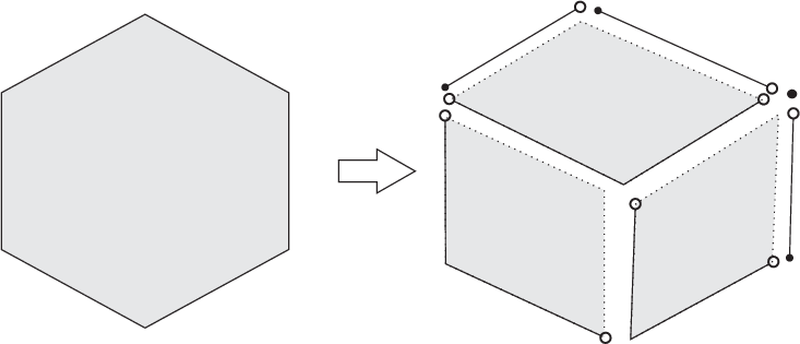
A zonotope decomposes in a disjoint union of semiopen bricks of dimensions ranging from $0$ to $n$.

Below we almost literally repeat the arguments from Section 3. Assume we have a convex zonotope $Z\subset\mathbb{R}^{n}$, that is, the Minkowski sum of linear segments $\{s_{i}\}_{i=1}^{m}$:

For each subset $I\subset[m]$ with $|I|\leq n$, which gives linearly independent $\{s_{i}\}_{i\in I}$, denote by $Z_{I}$ the semiopen brick spanned by segments $\{s_{i}\}_{i\in I}$. It is well-known that $Z$ can be partitioned into the union of all such $Z_{I}$, which implies immediately

where $\sharp(\cdot)$ denotes the number of integer points in a semiopen brick provided that the brick is spanned by linearly independent vectors. For linearly dependent vectors we set $\sharp:=0.$

References

- [1] M. Farber, Invitation to topological robotics, European Mathematical Society, 2008.
- [2] M. Farber and D. Schütz, Homology of planar polygon spaces, Geom. Dedicata, 125 (2007), 75-92.
- [3] A. Khovanskii, Newton polyhedra and toroidal varieties, Functional Analysis and Its Applications, 11(4):289–296, 1977.
- [4] A. Khovanskii and A. Pukhlikov, Finitely additive measures of virtual polytopes, St. Petersburg Math. J., Vol. 4, 2 (1993), 337-356.
- [5] G. Panina, Virtual polytopes and some classical problems, St. Petersburg Math. J., Vol. 14, 5 (2003), 823-834.
- [6] G. Panina, Moduli space of a planar polygonal linkage: a combinatorial description, arXiv:1209.3241
- [7] G. Panina, Cyclopermutohedron, Proceedings of the Steklov Institute of Mathematics, 2015, Vol. 288, 132-144.
- [8] G. Panina and I.Streinu, Virtual polytopes, Oberwolfach preprint OWP 2015-02.
- [9] A. Postnikov, Permutohedra, Associahedra, and Beyond, Int. Math. Res. Not. Vol. 6 (2009), 1026-1106.
- [10] B. Sagan, A note on Abel polynomials and rooted labeled forests, Discrete Mathematics, Vol. 44, 3 (1983), 293-298.
- [11] G.M. Ziegler, Lectures on polytopes, Graduate Texts in Mathematics. (Springer, Berlin 1995).