Entropy and diffuse scattering: comparison of NbTiVZr and CrMoNbV

Using hybrid MC/MD we pre-anneal structures of $N=128$ atoms (32 of each species) at T=1800K and then 1500K prior to lengthy data collection runs at 1200K. Our data collection runs extend for 15ps of molecular dynamics and 1500 attempted swaps for NbTiVZr, and 28ps of MD and 2800 attempted swaps for CrMoNbV. Acceptance rates for swaps indicate the similarity of chemical species in size and bonding preferences. Characteristically, the swap rates are lowest across the positive diagonal of periodic table squares [2] (i.e. Nb with Cr, and Zr with V) and highest along the negative diagonal (i.e. V with Mo, and ti with Nb). The relatively large acceptance rates for most pairs indicate the efficiency of our MC/MD method and suggest a likely large entropy of mixing.

Pair correlation functions are more revealing at lower temperature where atomic motion is reduced. To mimic an experiment where the alloy is formed at high temperature then cooled down, we quench from T=1200K down to 300K by performing molecular dynamics alone without Monte Carlo swapping. The chemical order remains characteristic of T=1200K even while the phonons equilibrate at 300K, as is the case in typical metallurgical experiments. Inspecting Fig. 1 note that CrMoNbV exhibits more ideal BCC structure at short range, with the nearest neighbor (NN) and next-nearest neighbor (NNN) peaks clearly resolved, than is the case for NbTiVZr, where these peaks are poorly resolved for Nb and V, and not resolved at all for Zr and Ti. Nonetheless, the long-range BCC structure is well preserved in both compounds as can be seen in the further neighbor peaks. A similar local instability was observed in ternary HfNbZr [4] which likewise mixes elements from the fourth and fifth periodic table columns (i.e. HEX and BCC ground states).

Because BCC is a loosely-packed structure, instantaneous atomic positions can be mapped back to the ideal BCC lattice sites that they are closest to. This allows us to uniquely identify NN and NNN bonds and report their statistics, as is done in Tables 1 and 2. Notice that the largest number of NN pairs occurs between the elements on the positive diagonals of the squares (Zr-V and Nb-Cr). This is reflected in Fig. 1 in the respective strengths of the peaks.

An instantaneous configuration is described by positions ${\bf r}_{m}$ that are displaced from the ideal lattice sites ${\bf R}_{m}$. We specify chemical occupation at position ${\bf r}_{m}$ by $c_{m}^{\alpha}$ defined as 1 if occupied by species $\alpha$ and 0 otherwise. The scattering amplitude at reciprocal space position ${\bf Q}$ is [5, 6, 7, 8]

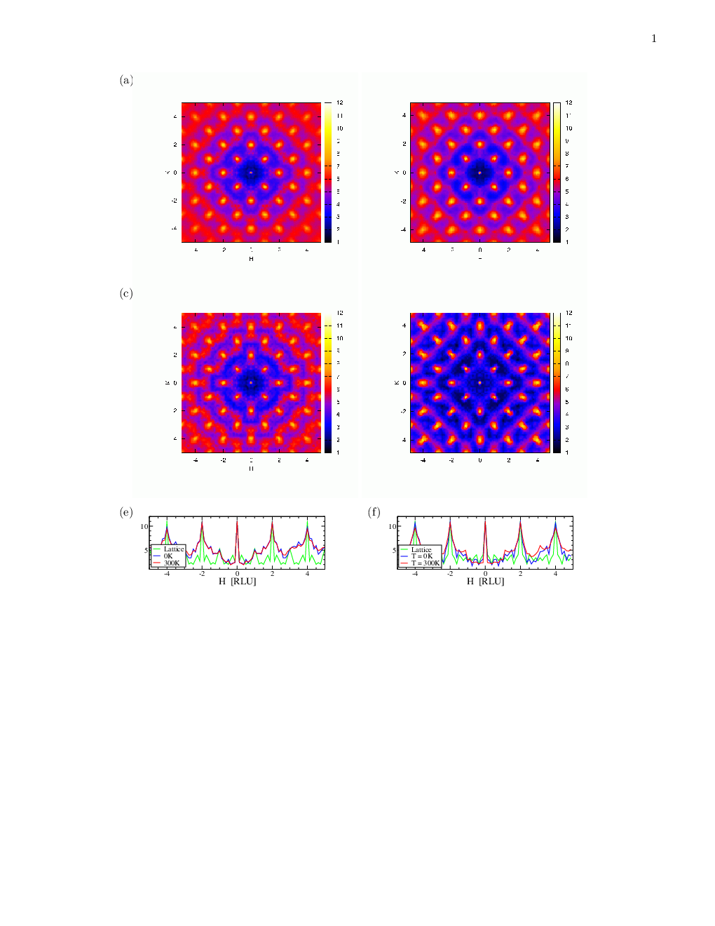
and its square is the scattering intensity $I({\bf Q})=|A({\bf Q})|^{2}$. Here $f_{\alpha}$ is the scattering form factor $f_{\alpha}$. For the present analysis we utilize x-ray form factors which we approximate as the atomic number, $f_{m}\approx Z_{m}$, independent of ${\bf Q}$. Note that the set of atomic numbers present in NbTiVZr (22, 23, 40 and 41) exhibits contrast similar to the set present in CrMoNbV (23, 24, 41, and 42). The natural logarithm of the intensity is plotted in Fig. 2, which is measured in reciprocal lattice units (RLU), $(2\pi/a)$, where $a$ is the conventional cubic lattice constant. Bragg peaks of the BCC lattices occur at ${\bf Q}={\bf G}=(2\pi/a)(H,K,L)$ where $H,K$ and $L$ are integers such that $H+K+L$ is even. For ${\bf Q}$ close to a Bragg peak ${\bf G}$ we shall denote the deviation by ${\bf k}={\bf Q}-{\bf G}$.

The average scattering intensity $I({\bf Q})=\langle|A({\bf Q})|^{2}\rangle$ separates into the Bragg component of the average lattice $I_{B}({\bf Q})=|\langle A({\bf Q})\rangle|^{2}$, and the diffuse part due to fluctuations $I_{D}({\bf Q})=\langle|A({\bf Q})-\langle A({\bf Q})\rangle|^{2}\rangle=I-I_{B}$. Owing to configurational fluctuations we take averages over both atomic displacements ${\bf u}_{m}={\bf r}_{m}-{\bf R}_{m}$ and chemical species fluctuations $\Delta c_{m}^{\alpha}=c_{m}^{\alpha}-c^{\alpha}$, yielding [7]

where we introduce the relative coordinates ${\bf R}_{mn}={\bf R}_{n}-{\bf R}_{m}$ and ${\bf u}_{mn}={\bf u}_{n}-{\bf u}_{m}$. For sufficiently small ${\bf Q}\cdot{\bf u}$, we may expand the exponential

Separating the diffuse scattering into components, we set $I_{D}=I_{0}+I_{1}+I_{2}+\cdots$, where each term arises from successively higher powers of ${\bf Q}\cdot{\bf u}$. Here $I_{0}$ reflects short-range chemical order, $I_{1}$ is known as the size effect, and $I_{2}$ includes both the thermal diffuse scattering due to lattice vibrations (phonons) and also the Huang scattering due to correlated lattice strains caused by differing atomic sizes.

To model chemical disorder, assume that all atoms sit on BCC lattice sites $\{{\bf R}_{m}\}$ with chemical species randomly distributed. For ${\bf Q}$ not on a Bragg peak, i.e. ${\bf k}={\bf Q}-{\bf G}\neq 0$, the sum over $m$ and $n$ in Eq. (2) simplifies to $I_{0}/N\sim\langle f^{2}\rangle-\langle f\rangle^{2}$ independent of ${\bf k}$, resulting in a uniform diffuse background. However, our neighbor statistics given in Tables 1 and 2 show the distributions of species is not fully random, but rather exhibits short-range correlations. Unlike species (e.g. Zr with V in NbTiVZr, or Nb with Cr in CrMoNbV) prefer to occupy nearest neighbor bonds. On a BCC lattice such sort-range chemical order can lead to partial B2-like ordering in which broad diffuse maxima arise at previously forbidden positions where $H+K+L$ is odd, as indeed we see in the case of NbTiVZr (Fig. 2(a)). Despite the short-range order present in CrMoNbV, we see no B2-like peaks in its diffraction pattern, which could indicate more complex order such as the B2₃ predicted in NbMo [9].

In fact, the atoms in our models do not sit at ideal lattice sites. The random distribution of unlike atomic sizes cause substantial relaxations off the lattice sites even at T=0K, and in addition they are subject to ordinary thermal fluctuations. Atomic size effects enter both at first and second order. At the first order the “atomic size effect” yields [8]

Nonvanishing $I_{1}$ depends on a correlation between the sign of ${\bf u}_{mn}$ and the strengths of the form factors at sites $m$ and $n$. The long-range displacement ${\bf u}_{mn}\sim{\bf e}_{{\bf R}}/R^{2}$ has Fourier transform ${\bf u}({\bf k})\sim{\bf e}_{{\bf k}}/k$. Thus close to a Bragg peak at ${\bf Q}={\bf G}+{\bf k}$, the size effect scattering diverges [7] as $I_{1}({\bf Q})\sim-{\bf G}\cdot{\bf e}_{\bf k}/k$ and will be asymmetric on the two sides of ${\bf G}$. For example, if atoms with large $f_{\alpha}$tend to move apart and small $f_{\alpha}$ tend to move closer, then $I_{1}$ is positive for negative ${\bf k}$ and negative for positive ${\bf k}$ [8]. This asymmetry can give the impression of a shift in the peak position [10].

At second order ordinary thermal diffuse scattering due to phonons, and also Huang scattering due to atomic sizes, both contribute diffuse scattering that diverges as $1/k^{2}$ in the vicinity of the Bragg peaks, each with its own characteristic angular distribution. Ordinary thermal fluctuations are characterized by phonons whose dispersion relations are of the form $\omega_{j}=c_{j}k$, where $j=1..3$ enumerate the independent modes of vibration whose polarization vectors are ${\bf e}_{j}({\bf k})$. The resulting diffuse intensity is proportional to [11]

As transverse sound speeds are typically less than longitudinal, the diffuse scattering will usually be stronger in directions ${\bf k}$ perpendicular to ${\bf G}$ than parallel to it. Such elongations can be seen in the diffuse pattern for CrMoNbV in surrounding the (200) and (400) peaks. Also visible are streaks running in [110] directions similar to those observed in other BCC metals [12]. These could indicate a low frequency phonon mode with a polarization component in the [110] direction. Notice that the streaks are stronger on the low ${\bf Q}$ side of the Bragg peaks (i.e. negative ${\bf G}\cdot{\bf e}_{\bf k}$) than on the high ${\bf Q}$ side, presumably as a result of the asymmetry of the size effect scattering $I_{1}$. In fact, there are local maxima of scattering in CrMoNbV that shift from, e.g. $H=3.1$ at $T=300$K to $H=3.5$ at $H=0$K, as can be seen in Fig. 2f indicating the diminishing contribution of the thermal component of $I_{2}$ relative to $I_{1}$.

Huang scattering arises from long-range strains arising from atomic size mismatch and hence is temperature independent. Originally derived for dilute impurities, a similar effect is present in concentrated alloys such as high entropy alloys. Because these strains are primarily longitudinal, only the component of ${\bf k}$ parallel to ${\bf G}$ enters, and the diffuse intensity is proportional to

which is equivalent to Eq. 5 setting ${\bf e}_{j}$ parallel to ${\bf k}$. The Huang scattering consists of figure-eights that are characteristically elongated in the longitudinal (radial) direction in reciprocal space. The low T patterns in Fig. 2 indeed show such elongation, and again the asymmetry in the sign of ${\bf k}$ arises from the contribution of $I_{1}$. The figure-eight pattern is not clearly resolved in the case of NbTiVZr, due to transverse strain that might indicate the presence of multisite correlations.

We evaluate the configurational entropy using the approach of the cluster variation method (CVM [13, 14]) by starting with the mean field (Bragg-Williams) entropy, then modifying it through the inclusion of factors that reduce the entropy by correcting for local correlations. First we define numerical values for symbols associated with the empty lattice, isolated points (P), near-neighbor bonds (NN), next-nearest-neighbor bonds (NNN), triangles (TRI) and tetrahedra (TET) as

where $M$ is the total number of lattice sites, $x_{\alpha}$ are the fractions of species $\alpha$, $y_{\alpha\beta}$ is the frequency of NN bonds between species $\alpha$ and $\beta$, etc. Next, we introduce combinatorial factors

Note that $\frac{1}{M}\log{\Omega_{P}}\approx-\sum_{\alpha}x_{\alpha}\log{x_{\alpha}}$ is the mean field entropy [15]. Multiplying $\Omega_{P}$ by $\Omega_{NN}$ reduces the entropy by an amount related to the deviation of NN bond frequencies $y_{\alpha\beta}$ from the uncorrelated frequency $x_{\alpha}x_{\beta}$. This level of approximation also goes by the name “quasichemical approximation” [16]. Multiplying instead by $\Omega_{NNN}$ would do the same for the NNN bonds, so the product $\Omega_{NN}\Omega_{NNN}$ given in Table 3 incorporates both effects, that is, it corrects the quasichemical approximation through inclusion of NNN correlations. Finally, including the remaining factor $\Omega_{TET}$ results in the conventional CVM entropy expression for BCC lattices [17].

By accumulating cluster occupation statistics during our MC/MD simulation, we are able to evaluate the numerical factors. Table 3 presents the resulting entropies (in the form of the phase space volume per site, which is the exponential of the entropy per site) for our two compounds. Note that these are configurational entropies only (i.e. no vibrational or electronic contributions), and that they reflect the chemical disorder at T=1200K. The entropies decrease monotonically as additional correlations are included. However, the CVM entropy must not be taken as an upper bound, because our sampling statistics are insufficient for the four point correlation function $z_{\alpha\beta\gamma\delta}$, and additional run time would increase this value. The proper values lie between NNN and CVM, and we recommend taking the NNN value as our best estimate. Interestingly, the entropy of NbTiVZr lies closer to the ideal (mean field) value than CrMoNbV does. This might reflect the extreme short-range disorder of NbTiVZr, which seemingly precludes establishing strong local chemical order.

References

• [1] O. N. Senkov, S. V. Senkova, D. B. Miracle, and C. Woodward, Mat. Sci. Eng. A 565, 51 (2013).
• [2] M. Widom, in High entropy alloys: fundamentals and applications, edited by M. Gao, J.-W. Yeh, P. Liaw, and Y. Zhang (Springer, 2015), chap. 8. Prediction of structure and phase transformations.
• [3] M. Widom, W. P. Huhn, S. Maiti, and W. Steurer, Mat. Met. Trans. A 45, 196 (2013).
• [4] W. Guo, W. Dmowski, J. Y. Noh, P. Rack, P. K. L. PK, and T. Egami, Mat. Trans. A 44, 1994 (2013).
• [5] B. Borie, Acta Cryst. 10, 89 (1957).
• [6] M. A. Krivoglaz, Diffuse Scattering of X-Rays and Neutrons by Fluctuations (Springer, 1996).
• [7] W. Schweika, Disordered Alloys: Diffuse SCattering and Monte Carlo simulations, vol. 141 of Springer Tracts in Modern Physics (Springer, Berlin, 1998).
• [8] T. R. Welberry, Diffuse X-Ray Scattering and Models of Disorder, vol. 16 of IUCR Monographs on Crystallography (Oxford, 2004).
• [9] V. Blum and A. Zunger, Phys. Rev. B 72, 02010R (2005).
• [10] B. E. Warren, B. L. Averbach, and B. W. Roberts, J. Appl. Phys. (1951).
• [11] T. Egami and S. J. L. Billinge, Underneath the Bragg Peaks, vol. 16 of Pergamon Materials Series (Elsevier, 2013).
• [12] I. B. Ramsteiner, O. Shchyglo, M. Mezger, A. Udyansky, V. Bugaev, S. Schoder, H. Reichert, and H. Dosch, Acta Mater. 56, 1298 (2008).
• [13] D. de Fontaine, in Solid State Physics, edited by H. Ehrenreich and D.Turnbull (Academic Press, 1979), vol. 34, pp. 73–274.
• [14] D. de Fontaine, in Solid State Physics, edited by H. Ehrenreich and D.Turnbull (Academic Press, 1994), vol. 47, pp. 33–176.
• [15] W. L. Bragg and E. J. Williams, Proc. Roy. Soc. London A 145, 699 (1934).
• [16] E. A. Guggenheim, Proc. Roy. Soc. London A 183, 213 (1944).
• [17] H. Ackermann, G. Inden, and R. Kikuchi, Acta Metall. 37, 1 (1989).