Finite-width Gaussian sum rules for pseudoscalar glueball based on correction from instanton-gluon interference to correlation function
Abstract
Based on correction from instanton-gluon interference to correlation function, the properties of the pseudoscalar glueball is investigated in a family of finite-width Gaussian sum rules. In the framework of semiclassical expansion for quantum chromodynamics in the instanton liquid background, the contribution arising from the the interference between instantons and the quantum gluon fields is calculated, and included in the correlation function together with pure-classical contribution from instantons and the perturbative one. The interference contribution is turned to be gauge-invariant, free of infrared divergence, and has a great role to restore the positivity of the spectra of the full correlation function. The negligible contribution from vacuum condensates is excluded in our correlation function to avoid the double counting. Instead of the usual zero-width approximation for the resonances, the usual Breit-Wigner form with a suitable threshold behavior for the spectral function of the finite-width resonances is adopted. A consistency between the subtracted and unsubtracted sum rules is very well justified. The values of the mass, decay width and coupling constants for the resonance in which the glueball fraction is dominant are obtained, and agree with the phenomenological analysis.
pacs
PACS-key11.55.Hx, 11.15.Kc, 12.38.Lg, 12.39.Mk1 Introduction
A significant issue in quantum chromodynamics (QCD) is to seek for the signal of the existence of glueballs. Because glueballs are bound sates composed of only gluons in the quarkless world, such signal may give a unique insight into the non-Abelian dynamics of QCD. Theoretical investigations including lattice simulations [1, 2, 3], model researches [4, 5, 6] and sum rule analyses [7, 8, 9, 10, 11, 12] have been going on for a long time, but no decisive evidence of the existence of glueballs has been confirmed by experimental research up to now [13, 14]. Further investigation on glueballs still makes sense.
One of the obstacles in theoretical researches of glueballs is that non-perturbative dynamics of QCD, which is responsible for the formation of hadrons, is difficult to handle, and the QCD vacuum is recognized to be a medium with complicated structure, and may impact greatly on the attributes of hadrons. In particular, the tunneling effect between the degenerate vacua of QCD should be taken into account. In the leading order, this effect is described by instantons [15, 16] and shown to be of great significance in generating the properties of the unusual hadrons, glueballs. Moreover, the glueball may be mixed with usual mesons of the same quantum numbers, making the identification of the glueball more complicated [12, 17].
Instantons, as the strong topological fluctuations of gluon fields in QCD, are widely believed to play an important role in the physics of the strong interaction (for reviews see [16, 18]). In particular, instantons provide mechanisms for the violation of both and chiral symmetry in QCD, and may therefore be important in determining hadron masses and in the resolution of the famous problem. Furthermore, it was recently shown that instantons persist through the deconfinement transition, so that instanton-induced interactions between quarks and gluons may underlie the unusual properties of the so called strongly coupled quark-gluon plasma recently discovered at RHIC [19].
In the instanton liquid model, a narrow sense describes the QCD vacuum as a sum of independent instantons with radius and effective density [20]. This model avoid the infrared problem caused by an infinite instanton density in the diluted gas model. The correctness of the instanton liquid model is still being intensively investigated. So far the model is essentially justified by its phenomenological success. The most important predictions are probably the breaking of the chiral symmetry (SBCS) in the axial triplet channel [21, 22] and the absence of Goldstone bosons in the axial singlet channel.
The non-perturbative effects of QCD is commonly casted into the description of non-perturbative vacuum, such as quark and gluon condensates and the instanton configurations. When contributions from both condensates and the instanton are included into the correlation function together, it leads to a double counting in a sense that they can be two alternative ways for parametrizing the nonperturbative vacuum [23, 24]. Moreover, the instanton distribution is closely connected with the vacuum condensates since the mean size and density of instantons can be deduced from the quark and gluon condensates, and conversely, the values of condensates can be reproduced from instanton distribution [25, 26, 27, 28]. The contributions of instanton and those of the condensates should be equivalent from each other in some case, and thus including both contributions at the same time will cause the double counting problem. To avoid it, many authors invoke some special techniques in dealing with the two contributions [29, 30, 31, 32]. This issue is, however, really not settled. Fortunately, the contribution of condensates to the correlation function in the glueball channels is unusually weak as demonstrated in this work and by many other authors[33, 34]. Therefore, it is assumed that the condensate contributions can be understood as a small fraction of the corresponding instanton one in the local limit. To prevent thoroughly from the problem of double counting, we choose to work in the instanton vacuum model of QCD, and carry out a semi-classical expansion in instanton background fields as suggested in our previous works to analyze the properties of the lowest scalar glueball [35, 36] and pseudoscalar one [37, 38], where the correlation function of the glueball currents are calculated by just including the contributions from the pure instantons, the pure quantum gluons, and the interference between both, instead of working with both instantons and condensates at the same time.
Zhang and Steele [39] have reported a disparity between their Laplace sum rule and Gaussian sum rule for the pseudoscalar glueball. In this reference, the optimized parameters of pseudoscalar glueball have been obtained from the Gaussian sum rule, while it fails to achieve a satisfying Laplace sum rule. This result seems strange, since both Laplace and Gaussian sum rules are derived from the same underlying dynamical theory, and should, at least, be approximately consistent. It reflects the inconsistency for including both condensate and instanton contributions in the correlation function and disregarding the important contribution from the interaction between instantons and their quantum counterparts at the same time.
An other serious problem in the glueball sum rule approach is that the fundamental spectral positivity bound is violated when including the strong repulsive pure instanton contribution, and as a consequence, the signal for the pseudoscalar glueball disappears[39]. To cure this pathology of positivity violation, the topological charge screening effect in the QCD vacuum is added to the correlation function, and a suitable instanton size distribution is taken into account[40, 7]. However, as comparing with the interference contribution, which we have recalculated in this paper, and the pure perturbative one in the considered energy region, the topological screening effect turns out to be negligible; and the pathology of positivity violation disappears when including the interference contribution (s. below).
Phenomenologically, the identification of the pseudoscalar glueball has been a matter of debate since the Mark II experiment proposed glueball candidates [41]. Later, in the mass region of the first radial excitation of the and mesons, a supernumerous candidate, the has been observed. It turns out to be clear that is allowed as glueball dominated state mixed with isoscalar states due to its behavior in production and decays, namely, it has comparably large branching ratios in the radiative decay, but not been observed in collisions[42, 13, 43]. A review on the experimental status of the is given in Ref. [13]. However, this state lies considerably lower than the theoretical expectations: the lattice QCD predictions suggest a glueball around GeV [44, 45]; the mass scale of the pseudoscalar glueball obtained in the QCD sum rule approach is above GeV [37, 38, 40, 7]. On the other hand, there are attractive arguments for the approximately degenerate in mass for the scalar and pseudoscalar glueballs [46], and even the scenario that a pseudoscalar glueball may be lower in mass than the scalar one is recently discussed in Ref. [47]. The possibly non-vanishing gluonium content of the ground state and mesons is discussed in [48, 49, 50, 12]. Up to now, only a topological model of the glueball as closed flux tube [46] predicts degeneracy of the and glueball masses and admits the region -GeV.
To face a more realistic phenomenological situation, we now reexamine the correlation function in the instanton liquid vacuum, and include all the resonances below and near the into the finite-width spectral function, and then achieve a series of results in traditional Gaussian sum rule analyses which are consistent with the phenomenology. On the other hand, as a crosscheck, these results are almost same with the Laplace ones (paper is submitted), because both Laplace and Gaussian sum rules are derived from the same underlying dynamical theory. The paper is organized as follows: In the second section, we present systematically the calculation of the contribution to the correlation function due to the interference between instantons and quantum gluons. It is this interference between instantons and quantum gluons to serve to be a mechanism to keep the positivity of the spectral function in contrast with the so-called topological charge screening effect stressed in Ref.[7]. The effect of the contribution of topological charge screening is found to be negligible as comparing with the interference one in the considered energy region. The spectral function is constructed in the similar way as in case of the glueball[36, 51] with a suitable threshold behavior in the third section. In the fourth section, a family of Gaussian sum rules are constructed. The numerical simulations are carried out in the fifth section, and the results are consistent with various Gaussian sum rules and in accordance with the phenomenology. Finally, the main conclusions are given, and a discussion of some interesting issues is open.
2 Correlation function
We are working in Euclidean QCD. The pseudoscalar glueball current is defined as
| (1) |
where is the strong coupling constant, is the gluon field strength tensor with the color index and Lorentz indices and , and
| (2) |
is the dual of . The current is a Lorentz-irreducible, gauge-invariant and local composite operator with the lowest dimension, and renormalization group invariant at least to the leading order in the quarkless world. It is noticed that the current is anti-hermitian due to the involving of the imaginary time, while its analytic continuation to the Minkowskian space-time is hermitian. The QCD correlation function is defined as
| (3) |
where is the hermitian conjugation of . The advantages to use the hermitian conjugation in definition are: first, the spectral functions both in Euclidean space-time and in its analytic continuation into Minkowskian space-time are, in principle, positively definite; and second, the relationship between the correlation functions both in Euclidean and Minkowskian formulations becomes very simple as
| (4) |
because the overall minus sign arising from the analytic continuation due to is just canceled with another minus sign arising from the mentioned different hermiticity of the pseudoscalar glueball current. Therefore, the expressions for and are, in fact, the same function of .
In the framework of semiclassical expansion, the glue potential field can be decomposed into a summation of the classical instanton and the corresponding quantum gluon field as
| (5) |
Consequently, the pure-glue Euclidean action can be expressed as
| (6) | |||||
where is the one-instanton contribution to the action, is the instanton field strength tensor
| (7) |
and the covariant derivative associated with the classical instanton field
| (8) |
In addition, the background field gauge
| (9) |
is used with being the corresponding gauge parameter, and certainly, the corresponding Faddeev-Popov ghosts according to the standard rule should be added to restore the unitarity. We note here that the structure constants should be understood as when any one of the color-indices , and is associated with an instanton field due to the property of the closure of any group.
According to the decomposition (5), the correlation function splits into three parts, namely the pure classical part, the pure quantum part and the interference part in the leading order
| (10) |
where the superscript indicates that it is calculated in the underlying dynamical theory, QCD. It is important to note that every part in rhs of (10) is gauge-invariant because the decomposition (5), in principle, has no impact on the gauge-invariance of the correlation function. The pure instaton contribution and the perturbative contribution up to three-loop level in the chiral limit of QCD are shown in Eqs. (80) and (81) respectively in Appendix A. The contribution of the topological charge screening which is not included in rhs of (10) is given in Appendix B.
One of our main tasks in this work is to calculate the contribution in (10), which is arising from the interference between the classical instantons and quantum gluons in the framework of the semi-classical expansion for QCD with the instanton background. After imposing the background covariant Feynman gauge () for the quantum gluon fields, we are still free to choose a gauge for the background field . In the following, the singular gauge is chosen to the non-perturbative instanton field configurations as
| (11) |
with
| (12) |
and the corresponding field strength tensor is
| (13) | |||||
with and denote respectively the center and size of the instanton, called collective coordinates together with the color orientation, and is the ’t Hooft symbol which should be replaced with the anti-’t Hooft one for an anti-instanton field. For the sake of simplicity, in the practice the most used is the spike size distribution , where is the overall instanton density and is the average instanton size. The fact that the strong coupling constant emerging in the denominator of the rhs of (11) reveals the nonperturbative nature of these classical configurations. In fact, instantons play quite important role in QCD sum rule. Early QCD sum rules neglecting instanton-induced continuum contributions didn’t obtain reliable results in many cases, but they are then solved by including such instanton-induced effects [30, 9].
Before starting with the contraction between the quantum fields, we note that the time-development of the instanton vacuum produces the pre-exponential factor for the distribution of the instantons[52, 15, 53], and is understood as taking ensemble average over the collective coordinates besides taking the usual vacuum expectation value due to the separation (5)
| (14) |
where the super index ’(int)’ indicates the corresponding quantity containing only the interference part between the quantum and classical ones. Using the spike distribution, (14) becomes
| (15) |
where the factor 2 comes from the mutually equal contributions of both instanton and anti-instanton. Next important step is to specify the form of the gluon propagator which in the background field Feynman gauge can be read from the part of quadratic in [54, 55]
| (16) | |||||
with . Keeping only terms proportional to , one has[56]
| (17) |
where the first term in rhs of the above equation is the pure-gluon propagator in the usual Feynman gauge, and the second and third ones are the leading contribution of the instanton field to the gluon propagator. For short distance region, we assume that the contribution from a single instanton is dominant over multi-instantons[57]. At the leading loop level, the gluon propagator (17) becomes the pure-gluon one.
In calculation, we expand the current into terms which are the products of quantum gluon fields and their derivatives with coefficients being composed of the instanton fields
| (18) |
where the operators in terms of instanton and quantum gluon fields are listed in Appendix C. Eq.(15) can be rewritten as
| (19) |
where the denotes the contributions from the products of operators being proportional to , and the expressions of in terms of are shown in Appendix D. The corresponding twelve kinds of Feynman diagrams as shown in the FIG. 1, where the contributions from the first three diagrams are of the order of , and the contributions of the remainders are superficially of the order of , and those from the diagrams (4),(5) and (6), in fact, are vanishing because of violating the conservation of the color-charge, namely
| (20) |


Now, we are in the position to evaluate the contributions of the remainder diagrams in FIG. 1. Using the standard technique to regularizing the ultraviolet divergence in the modified minimal subtraction scheme, the result for the interference part of the correlation function is
| (21) | |||||
where we have ignored terms being proportional to the positive powers of which vanish after Borel transformation, and the dimensionless coefficients are numerically determined to be
| (22) |
through a tedious calculation. It should be noted that there is no infrared divergence as expected by the instanton size being fixed in the liquid instanton vacuum model. Comparing Eq.(21) with our previous result [37, 38], they differ not only in some coefficients but also in the logarithms structures due to the fact that the newly improved calculation is free of infrared divergence while our old one were not, and it would need a corresponding cutoff to regularize the integral in the infrared limit.
Putting everything above together, our final correlation function for the pseudoscalar glueball current is of the form
| (23) | |||||
with .
Before going on, let us compare the roles of the various parts of the contributions in correlation function. The imaginary part of the correlation function (23) can be worked out to be
| (24) | |||||
where the pure classical contribution (the first term on rhs of (24)) is most dominant, and the contribution of the interference terms (the second term on rhs) is of the second place, the pure perturbative contribution simply plays the role of the third place, as shown in FIG. 2 where the imaginary part of the correlation function is multiplied with a weight function as required by the Gaussian sum rules, and in accordance with the spirit of the semiclassical expansion. All these three contributions are positively definite as expected. We note that the contribution from the topological charge screening, from (84), is displayed in FIG. 2 as well, and its role is almost insignificant. Moreover, it is easy to see from FIG. 2 that the imaginary part of the correlation function is already positive from to without including the contribution of the topological charge screening, and the so-called positivity problem is no longer there. Therefore, the interference contribution to the correlation function is significant important not only in its magnitude but also in restoring the positivity to the spectral function.
We note here that the so-called condensate contribution to the correlation function of the pseudoscalar glueball current is proven to be very small in comparing with the one of (23), as shown in Appendix E, where the comparison between the real and imaginary parts of the correlation function and condensate contribution to it are made, and shown in FIG. 8 and 9. For the reasons given above, the contributions from the topological charge screening effect and the usual condensates are omitted in our sum rule analysis.

3 Spectral function
In the isosinglet channel there are five gauge-invariant composite operators with the quantum numbers of which are bilinear in the fundamental quark, antiquark and gluon fields, namely the pseudoscalar quark densities, the divergences of the axial quark currents and the gluon anomaly:
| (25) |
| (26) |
| (27) |
where is the flavor Gell-Mann matrix, and with being the flavor unit matrix. Only three of these operators are independent due to the two renormalization-invariant axial Ward identities
| (28) | |||||
| (29) | |||||
Further, under renormalization and the flavor space rotation, we have
| (30) |
| (31) |
| (32) |
where the quantities with subscript are the renormalized ones. As a consequence, the gluon anomaly operator even through renormalization-invariant in the pure gluon world, is a linear combination of three operators , and after renormalization. Therefore, one assumes that there may be some isosinglet quark-antiquark pseudoscalar states mixed with the pseudoscalar glueball ground state G.
Now we construct the spectral function for the correlation function of the pseudoscalar glueball current. The usual lowest one resonance plus a continuum model is used to saturate the phenomenological spectral function:
| (33) |
where is the QCD-hadron duality threshold, the step function and the spectral function for the lowest pseudoscalar glueball state. In the usual zero-width approximation, the spectral function for a single resonance is assumed to be
| (34) |
where is the mass of the lowest glueball, and is the coupling constant of the current to the glueball defined as
| (35) |
The threshold behavior for is known to be
| (36) |
from the low-energy theorem in the world of no light quark flavors [58] or the one in the world with three light flavors and [59]. In fact, the threshold behavior (36) is only proven to be valid near by the chiral limit; it may not be extrapolated far away. Therefore, instead of considering the coupling as a constant [7], we choose a model for as
| (37) |
where the and are some constants determined late in numerical simulation.
To go beyond the zero-width approximation, in facing the near-actual situation, the Breit-Wigner form for a single resonance is assumed for
| (38) |
where is the width of the lowest glubeball.
Further, the one isolated lowest resonance assumption is questioned from the admixture with quarkonium states, and it is known from the experimental data that there are five pseudoscalar resonances till and around the mass scale of 1.405 GeV (namely , , , and ). The form of the spectral function for five resonances is taken to be
| (39) |
where and being the mass and width of the i-th resonance, respectively. For the sake of simplicity, all coupling constants for are fixed with the same as shown in (37).
It is noticed that there are other pseudoscalar resonances and which are omitted from the summary table of PDG. These two resonances are excluded in our consideration. The reasons may be listed in order: First, although and may certainly be coupled to the pseudoscalar glueball current via the gluon anomaly, such coupling, however, contains a factor of the running coupling as commonly seen in QCD, and becomes weaker with increases, as demonstrated in an effective QCD low energy theory [60]. Second, the mixing between the considered pseudoscalar glueball and and is believed to be very small because the locations of and are far away from the scale of the lowest pseudoscalar glueball. Third, the continuum threshold , determined in our sum rule approach, is only in an effective sense due to the accuracy level of the present calculation.
4 Finite width Gaussian sum rules
In this section, we construct the appropriate sum rules of pseudoscalar glueball current which has the form due to dispersion relation
| (40) |
where could be simulated by the phenomenological one whithin an assumed model of the spectral function in a spirit of sum rule approach. Using the Borel transformation [61]
| (41) |
to both sides of (40), a family of Gaussian sum rules can be formed to be [61]
| (42) | |||||
where is the continuum threshold which hadronic physics is (locally) dual to QCD above it.
| (43) |
comes from the low-energy theorem for QCD with three light flavors[59], and
| (44) |
for the phenomenological contributions to the sum rules, and
| (45) |
for the theoretical contributions, where is the contribution of continuum being defined as
| (46) |
and is defined as
| (47) | |||||
Substituting the correlation function (23) of pseudoscalar glueball into (47), one can derive the Gaussian sum rules of and
| (48) | |||||
| (49) | |||||
| (50) | |||||
where
| (51) |
and parabolic cylinder function defined as
| (52) |
5 Numerical simulation
The expressions for the three-loop running coupling constant with three massless flavors at renormalization scale [62]
| (53) |
are used, where is the two-loop running coupling constant with
| (54) |
and
| (55) |
with the color number and the QCD renormalization invariant scale . We take after calculating Borel transforms based on the renormalization group improvement for Gaussian sum rules [63]. The subtraction constant has been fixed as [7]
| (56) |
and the values of the average instanton size and the overall instanton density are adopted from the instanton liquid model[25]
| (57) |
The resonance parameters in Eq.(39) could be estimated by matching both sides of sum rules Eq.(42) optimally in the fiducial domain. In doing so, the parameter and the threshold should be determined priority. Firstly, it is obvious that must be greater than the mass square of the highest lying isolated resonance considered, namely
| (58) |
in our multi-resonance assumption (or just the resonance mass itself in the case of a single resonance assumption), and should guarantee that there is a sum rule window for Gaussian sum rules. Secondly, the peak positions of versus curves should not change too much with moderate variation of . Here we do not mention about the values of in this condition, because the peak positions of these curves is not affected by appropriate values of . It is found that the behavior of these curves can satisfy above requirements as shown in FIG. 3 if lies in the interval of . It is also remarkable that the peak positions has already indicated the approximate mass of the hadron considered. Thus, we would expect that the mass of the pseudoscalar glueball should be nearby the value . In another way, if one uses the curves of versus with fixed and to obtain the physical parameters through (43), then should be set approximately to be of the curves of versus , so as to highlight the underlying hadron state in consideration and suppress the contributions from other states.

Besides, it needs a sum rule window which the hadron physical properties should be stable in this region. For the upper limit of the sum rule window, the resonance contribution should be great than the continuum one
| (59) |
according to the standard requirement due to the fact that in the energy region above the perturbative contribution is dominant. At , which lies in the low-energy region, we require that the single instanton contribution should be relatively large so that
| (60) |
In the same time, to require that the multi-instanton corrections remain negligible, we simply adopt a rough estimate
| (61) |
According to the above requirements, we find that in the domain
| (62) |
our sum rules work very well. Finally, in order to measure the compatibility between both sides of the sum rules (42) in our numerical simulation, we divide the sum rule window into segments of equal width, , with and , and introduce a variation (called the matching measure) which is defined as
| (63) |
where and are lhs and rhs of (42) evaluated at .
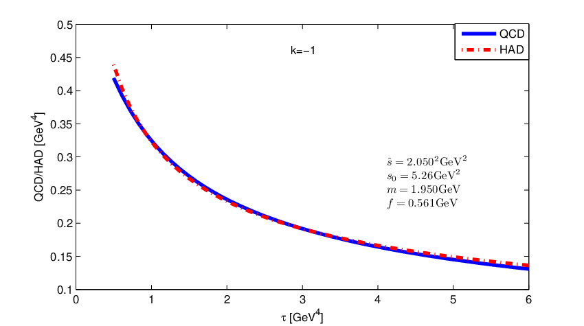
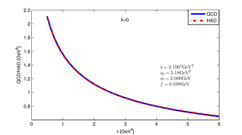
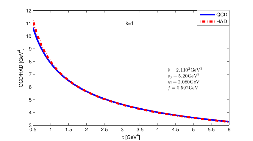
Let us first consider the case of single-resonance plus continuum model (34) of the spectral function by excluding the interference contribution from (the case A), in order to recover the results before. In this case, the imaginary part of , however, becomes negative for below , and the full interaction plays a role of repulsive potential in the pseudoscalar channel. This is the reason why the authors in Ref. [39] cannot find the signal for the pseudoscalar glueball. When we chose to work in the positively definite region, say , The mass of the glueball can be worked out by using the family of Gaussian sum rules (42). The fitting parameters are listed in the first three lines of Tab. 1 and the corresponding matching curves for , and are displayed in FIG. 4, respectively. The optical values of mass, coupling constant and of pseudoscalar glueball are
| (64) |
where the errors are estimated from the uncertainties of the spread between the individual sum rules, and by varying value of in the region of (the same for hereafter)
| (65) |
The mass values of pseudoscalar glueball in (64) are reasonably consist with the one obtained in Ref. [7] by adding the topological charge screening effect and performing the so-called Gaussian-tail distribution for instanton size. However, after performing the Gaussian-tail distribution for instanton size, the mass of the glueball is lower to be around [7] in contradiction with the lattice simulation [64, 45] and phenomenology [65]. The mass scales in (64) locate at the strong repulsive potential region of energy (below ) where the bound state of glueball cannot form when working in the spike distribution which is motivated from the liquid instanton model of QCD vacuum in the large limit. In fact, the fundamental spectral positivity bound can be traced back to the definition of the correlation function (3). The spectral function should be positive even before taking the average with any specific instanton-size distribution. It is difficult for us to understand that there is no artificial in changing the positivity behavior of the spectral function just by performing the average with the Gaussian-tail distribution for the instanton size.
From now on, the full correlation function including the interference contribution , (23), is used in our analysis of the Gaussian sum rules (42). In the case of single-resonance plus continuum models, specified respectively by (34) and (38), for the spectral function, the optimal parameters governing the sum rules with zero (the case B) and finite (the case C) widths are listed from the fourth to ninth line of Tab. 1 and the corresponding curves for the lhs and rhs of (42) with , and are displayed in FIG. 5 and 6 respectively. From Tab. 1, the optical values of the pseudoscalar glueball mass, width, coupling and the duality threshold with the best matching are:
| (66) |
for one zero-width resonance model, and
| (67) |
for one finite-width resonance model. It is shown in FIG. 5 that the topological charge screening effect has little impact on Gaussian sum rules indeed.
In the numerical simulation for the case of the five finite-width resonances plus continuum model (39) for the spectral function (the case D), we just choose the data in PDG as the fitting parameters for masses and width of the resonances , , and , and the result of the single resonance model (the case C) as the fitting parameters for ; while the couplings of the five resonances to the current are chosen to be approximately the same as that for determined in case C because the pseudoscalar qurkonia can be directly coupled to the gluon anomaly, and as a consequence, all five resonances should be coupled to the current with the strengths of almost the same magnitude of degree; finally, the optimal parameters are determined by adjusting the chosen parameters so that the matching measure for both sides of the Gaussian sum rules (42) is minimal. The optimal parameters governing the sum rules are listed in the remaining lines of Tab. 1. The corresponding curves for the lhs and rhs of (42) with , and are displayed in the FIG. 7. Taking the average, the optical values of the widths of the five lowest resonances in the world of QCD with three massless quarks, and the corresponding optical fit parameters are predicted to be
| (68) |
| (69) |
| (70) |
| (71) |
| (72) |
with
| (73) |
The FIG. 6 and 7 show the satisfactory compatibility between both sides of the sum rules over the whole fiducial region. These results are in good accordance with the experimental discovered resonance [14]
| (74) |
| case | resonances | |||||||||
|---|---|---|---|---|---|---|---|---|---|---|
| 0 | 0.561 | |||||||||
| A | 0 | 0.599 | ||||||||
| 0 | 0.592 | |||||||||
| 0 | 1.457 | |||||||||
| B | 0 | 1.387 | ||||||||
| 0 | 1.392 | |||||||||
| 0.05 | 1.630 | |||||||||
| C | 0.08 | 1.671 | ||||||||
| 0.03 | 1.760 | |||||||||
| D | 1.100 | |||||||||
| 1.100 | ||||||||||
| 0.055 | 1.200 | |||||||||
| 0.051 | 1.330 | |||||||||
| 0.085 | 1.010 | |||||||||
| 1.200 | ||||||||||
| 1.300 | ||||||||||
| 0.055 | 1.195 | |||||||||
| 0.051 | 1.300 | |||||||||
| 0.085 | 1.011 | |||||||||
| 1.100 | ||||||||||
| 1.200 | ||||||||||
| 0.055 | 1.210 | |||||||||
| 0.051 | 1.310 | |||||||||
| 0.085 | 1.050 | |||||||||


6 Discussion and Conclusion
The instanton-gluon interference and its role in finite-width Gaussian sum rules for pseudoscalar glueball are analyzed in this paper. Our main results can be summarized as follows:
First, the contribution to the correlation function arising from the interference between the classical instanton fields and the quantum gluon ones is reexamined and derived in the framework of the semi-classical expansion of the instanton liquid vacuum model of QCD. The resultant expression is gauge invariant, and free of the infrared divergence, and differs from our previous one not only in some coefficients but also in the logarithms structures[37, 38]. Its magnitude is just between the larger contribution from pure classical instanton configurations and the smaller one from the pure quantum fields, and plays a great role in sum rule analysis in accordance with the spirit of semi-classical expansion. The imaginary part of the correlation function including this interference contribution turns to be positive without including of the topological charge screening effect which is proven to be smaller than the perturbative contribution in the fiducial sum rule window, and negligible in comparison with the interference effect. The so-called problem of positivity violations in the imaginary part of the correlation function, stressed by H. Forkel[7], disappears. Moreover, it is excluded in the correlation function the traditional condensate contribution to avoid the double counting[7] because condensates can be reproduced by the instanton distributions[25, 26, 27, 28]; Another cause to do so is that the usual condensate contribution is proven to be unusually weak, and cannot fully reflect the nonperturbative nature of the low-lying gluonia[66, 7, 37, 38]; In our opinion, the condensate contribution can be considered as a small fraction of the corresponding instanton one, so it is naturally taken into account already.
Second, the properties of the lowest lying pseudoscalar glueball are systematically investigated in a family of Gaussian sum rules in five different cases. In case A, the correlation function contains only pure perturbative contribution and pure instanton one, and a single zero-width resonance plus continuum model is adopted for the spectral function, and of course, the old results are recovered (even excluding the topological charge screening contribution), and some pathology is explored. To go beyond the above constraint, all the contributions arising from pure instanton, pure perturbative and interference between both are included in the correlation function for cases B, C and D, in which a single zero-width resonance plus continuum model of the spectral function is adopted for case B, and a single finite-width resonances plus continuum model for case C, and the five finite-width resonances plus continuum model for case D, respectively. The optimal fitting values of the mass , width , coupling constant , continuum threshold for the possible resonances are obtained, and quite consistent with each other. The main difference between this work and our previous one[37, 38] is that for the spectral function of considered resonances, instead of the zero-width approximation of one gluonic resonance plus another low-lying quark-antiquartk ones, the finite-width Breit-Wigner form with a correct threshold behavior for the lowest five resonances with the same quantum numbers is used in this work in order to compare with the phenomenology. The resultant Gaussian sum rules with are carried out with a few of the QCD standard inputting parameters, and really in accordance with the experimental data.
As a discussion, let us now identify where the lowest lying pseudoscalar glueball is. The result of the single-resonance plus continuum models B and C, namely Eqs. (66) and (67), imply that the meson may be the most fevered candidate for the lowest lying pseudoscalar glueball because the difference between the two models is just the width of the resonances, and the latter is of course believed to be more in accordance with the reality. This conclusion can further be justified by the result of the five-resonances plus continuum model, namely Eqs. (71), (72) and (73). Note that the first two resonances and are far away from the mass scale of , and usually considered as the superposition of the fundamental flavor-singlet and octet pseudoscalar mesons composed of quark-antiquark pair to have a dominant role in responsible for the axial anomaly[67, 68, 69]. In order to explore the structures of the remainder three resonance , and , we would like use the -- mixing formalism based on the anomalous Ward identity for transition matrix elements[49, 12] to relate the physical states , and to the fundamental flavor-singlet and octet quark-antiquark mesons and the lowest pure gluon state through a rotation
| (75) |
where the is the mixing matrix [12, 49]
| (76) |
where and is [49] mixing angle and the mixing angle of the pseudoscalar glueball with . Then, one has
| (77) |
To be quantitative, the corresponding normalized couplings to the three resonances , and G with masses 1.295, 1.475, 1.405 GeV can be read from Tab. 1 to be
| (78) |
after normalization, respectively. As a relatively rough estimation, from Eq. (78) the values of the couplings of to the states , and pseudoscalar glueball are obtained
| (79) |
by reversing Eq. (75). This shows that the coupling of the glueball current to the pure glueball state is dominant, and the signs of the couplings and are similar to those predicted by the scalar glueball-meson coupling theorems [70, 58].
Furthermore, and could originate from a single pole (see Amsler and Masoni’s review for eta(1405) in PDG). To check whether the single pseudoscalar meson assumption may be consistent with our sum rule approach, or the dependence of the results on the model selected for the spectral function, we add an analysis of four resonance model for the spectral function. The result is shown in Appendix F. From FIG. 10 and Tab. 2 where it is easy to see that the four resonance model for the spectral function is inconsistent with our sum rule analysis because, firstly the resultant mass scale of the fourth resonance is approximately in average which locates outsides of the sum rule window; secondly the match degree of the four resonance model is obviously worse than the of the five resonance model.
In summary, our result suggests that is a good candidate for the lowest pseudoscalar glueball with some mixture with the nearby excited isovector and isoscalar mesons. This is a first theoretical support for the phenomenological estimation from the sum rule approach.
Acknowledgements
This work is supported by BEPC National Laboratory Project R&D and BES Collaboration Research Foundation.
Appendix A Pure instanton and perturbative contribution
In instanton liquid model, the pure instanton contribution of pseudoscalar glueball with spike instanton distribution in Euclidean space-time is known as[7, 71, 72, 73]
| (80) |
where is the McDonald functions and is the size distribution of instantons, and the appearance of the overall minus sign in rhs of (80) is due to the anti-hermitian property of the current, i.e. in Euclidean space-time.
The second part of (10) has already been calculated up to three-loop level in the dimensional regularization scheme[11, 71, 74]
| (81) | |||||
where is the renormalization scale, and the coefficients with the inclusion of the correct threshold effect are
| (82) |
for QCD with three massless quark flavors up to three-loop level.
Appendix B Topological charge screening
The topological charge screening effect can be understood by tracing back to the anomaly of the axial-vector current with being quark field of flavor
| (83) |
where the topology charge current relates to the pseudoscalar glueball current as . Eq. (83) indicates that instantons generate quark-antiquark pairs, which then may form a light meson to mediate the long-range multi-instanton interaction [16]. Kikuchi and Wudka [75] suggest that such a light meson, which can couple to the instanton in the way that the instanton generates all light quark flavors with the identical probability, be the meson , and constructs an effective Lagrangian (see also [76, 77]) which gives rise to the topological charge screening contribution to the correlation function of the pseudoscalar current as[7]
| (84) |
where and are the masses of the mesons and , and the two constants and are evaluated to be and , and and are the coupling strength of to an instanton and the mixing angle, respectively.
Appendix C The operators
The operators in terms of instanton and quantum gluon fields are
| (85) |
where is the instanton field strength associated with the instanton field .
Appendix D The interference contributions
The expressions of the interference contributions in terms of are
| (86) | |||||
where
| (87) |
Appendix E Comparison between the condensate contributions and the instanton-induced ones
The contributions arising from condensates up to the eighth dimensions are known to be as follows [7]
| (88) | |||||
where
| (89) |
The imaginary part of condensates (88) has the form
| (90) | |||||
The comparison between the imaginary part of the correlation function, (24), and condensate contribution to it are shown in FIG. 8, while the comparison between the various real parts of (23) (which altogether are related with the imaginary part by the dispersion relation (40)) and condensate contribution to it are shown in FIG. 9.


Appendix F The results for the four finite-width resonance model from the Gaussian sum rules
The optimal parameters of the four finite-width resonance model for the spectral function are listed in Tab 2, and the corresponding plots are shown in FIG. 10.
| resonances | |||||||||
| 0.548 | 1.100 | ||||||||
| 0.958 | 1.100 | 5.30 | |||||||
| 1.295 | 0.055 | 1.200 | |||||||
| 1.412 | 0.051 | 1.340 | |||||||
| 0.548 | 1.200 | ||||||||
| 0.958 | 1.300 | 4.80 | |||||||
| 1.295 | 0.055 | 1.195 | |||||||
| 1.420 | 0.051 | 1.670 | |||||||
| 0.548 | 1.100 | ||||||||
| 0.958 | 1.200 | 4.29 | |||||||
| 1.295 | 0.055 | 1.210 | |||||||
| 1.410 | 0.051 | 1.740 | |||||||


References
- [1] Apoorva Patel, Rajan Gupta, Gerald Guralnik, Gregory W. Kilcup, and Stephen R. Sharpe. An Improved Estimate of the Scalar Glueball Mass. Phys.Rev.Lett., 57:1288, 1986.
- [2] A. Vaccarino and D. Weingarten. Glueball mass predictions of the valence approximation to lattice QCD. Phys.Rev., D60:114501, 1999.
- [3] Xiang-Fei Meng, Gang Li, Ying Chen, Chuan Liu, Yu-Bin Liu, et al. Glueballs at finite temperature in SU (3) Yang-Mills theory. Phys.Rev., D80:114502, 2009.
- [4] Nathan Isgur, Richard Kokoski, and Jack E. Paton. Gluonic Excitations of Mesons: Why They Are Missing and Where to Find Them. Phys.Rev.Lett., 54:869, 1985.
- [5] A.V. Anisovich, V.V. Anisovich, and A.V. Sarantsev. glueball/ state mixing in the mass region near 1500-MeV. Phys.Lett., B395:123–127, 1997.
- [6] M. Albaladejo and J.A. Oller. Identification of a Scalar Glueball. Phys.Rev.Lett., 101:252002, 2008.
- [7] Hilmar Forkel. Direct instantons, topological charge screening, and qcd glueball sum rules. Phys. Rev. D, 71:054008, Mar 2005.
- [8] Jue-Ping Liu and Dun-Huan Liu. The Leading quark mass corrections to the QCD sum rules for the scalar glueball. J.Phys., G19:373–387, 1993.
- [9] T. Schäfer and E. V. Shuryak. Glueballs and instantons. Phys. Rev. Lett., 75:1707–1710, Aug 1995.
- [10] Leonard S. Kisslinger and Mikkel B. Johnson. Scalar mesons, glueballs, instantons and the glueball/sigma. Phys.Lett., B523:127–134, 2001.
- [11] D. Harnett and Thomas G. Steele. A Gaussian sum rules analysis of scalar glueballs. Nucl.Phys., A695:205–236, 2001.
- [12] Hai-Yang Cheng, Hsiang-nan Li, and Keh-Fei Liu. Pseudoscalar glueball mass from -- mixing. Phys. Rev. D, 79:014024, Jan 2009.
- [13] A. Masoni, C. Cicalo, and G.L. Usai. The case of the pseudoscalar glueball. J.Phys., G32:R293–R335, 2006.
- [14] V. Crede and C.A. Meyer. The Experimental Status of Glueballs. Prog.Part.Nucl.Phys., 63:74–116, 2009.
- [15] G. ’t Hooft. Computation of the quantum effects due to a four-dimensional pseudoparticle. Phys. Rev. D, 14:3432–3450, Dec 1976.
- [16] T. Schäfer and E. V. Shuryak. Instantons in qcd. Rev. Mod. Phys., 70:323–425, Apr 1998.
- [17] Vicente Vento. Scalar glueball spectrum. Phys. Rev. D, 73:054006, Mar 2006.
- [18] Dmitri Diakonov. Instantons at work. Prog.Part.Nucl.Phys., 51:173–222, 2003.
- [19] E.V. Shuryak. Strongly Coupled Quark-Gluon Plasma: The Status Report. pages 3–16, 2006.
- [20] Ernst-Michael Ilgenfritz and M. Muller-Preussker. Statistical Mechanics of the Interacting Yang-Mills Instanton Gas. Nucl.Phys., B184:443, 1981.
- [21] Dmitri Diakonov and V. Yu. Petrov. Instanton Based Vacuum from Feynman Variational Principle. Nucl.Phys., B245:259, 1984.
- [22] Dmitri Diakonov and V. Yu. Petrov. A Theory of Light Quarks in the Instanton Vacuum. Nucl.Phys., B272:457, 1986.
- [23] Stephan Narison. Light and heavy quark masses, flavor breaking of chiral condensates, meson weak leptonic decay constants in QCD. 2002.
- [24] Stephan Narison and Valentin I. Zakharov. Hints on the power corrections from current correlators in x space. Phys. Lett., B522:266–272, 2001.
- [25] Edward V. Shuryak. The Role of Instantons in Quantum Chromodynamics. 2. Hadronic Structure. Nucl.Phys., B203:116, 1982.
- [26] Dmitri Diakonov and V. Yu. Petrov. Chiral condensate in the instanton vacuum . Phys.Lett., B147:351–356, 1984.
- [27] C. Edwards et al. Identification of a pseudoscalar state at 1440 mev in radiative decays. Phys. Rev. Lett., 49:259–262, Jul 1982.
- [28] Jue-Ping Liu and Ping-Xiong Yang. Temperature dependence of three gluon condensates in the instanton medium. J.Phys., G21:751–764, 1995.
- [29] Derek B. Leinweber. QCD sum rules for skeptics. Annals Phys., 254:328–396, 1997.
- [30] Hilmar Forkel. Scalar gluonium and instantons. Phys. Rev. D, 64:034015, Jul 2001.
- [31] Zhu-feng Zhang and Hong-ying Jin. Instanton Effects in QCD Sum Rules for the Hybrid. Phys. Rev., D85:054007, 2012.
- [32] Hee-Jung Lee and N. I. Kochelev. On the pi pi contribution to the QCD sum rules for the light tetraquark. Phys. Rev., D78:076005, 2008.
- [33] V. A. Novikov, Mikhail A. Shifman, A. I. Vainshtein, and Valentin I. Zakharov. eta-prime Meson as Pseudoscalar Gluonium. Phys. Lett., B86:347, 1979. [Pisma Zh. Eksp. Teor. Fiz.29,649(1979)].
- [34] Stephan Narison. Masses, decays and mixings of gluonia in QCD. Nucl. Phys., B509:312–356, 1998.
- [35] Zhenyu Zhang and Jueping Liu. Stabilization and consistency for subtracted and unsubtracted QCD sum rules for scalar glueball. Chin.Phys.Lett., 23:2920–2923, 2006.
- [36] Shuiguo Wen, Zhenyu Zhang, and Jueping Liu. scalar glueball in finite-width gaussian sum rules. Phys. Rev. D, 82:016003, Jul 2010.
- [37] Chuanfeng Xian, Feng Wang, and Jueping Liu. Consistent Laplace sum rules for pseudoscalar glueball in the instanton vacuum model. Eur.Phys.J.Plus, 128:115, 2013.
- [38] Chuanfeng Xian, Feng Wang, and Jueping Liu. Gaussian sum rules for glueball in the instanton vacuum model. J.Phys., G41:035004, 2014.
- [39] Ai. lin Zhang and Thomas G. Steele. Instanton and higher loop perturbative contributions to the QCD sum rule analysis of pseudoscalar gluonium. Nucl.Phys., A728:165–181, 2003.
- [40] Hilmar Forkel. Topological charge screening and pseudoscalar glueballs. Braz.J.Phys., 34:875–878, 2004.
- [41] D.L. Scharre, G. Trilling, G.S. Abrams, M.S. Alam, C.A. Blocker, et al. Observation of the Radiative Transition . Phys.Lett., B97:329, 1980.
- [42] Vincent Mathieu, Nikolai Kochelev, and Vicente Vento. The Physics of Glueballs. Int.J.Mod.Phys., E18:1–49, 2009.
- [43] M. Acciarri et al. Light resonances in and final states in collisions at LEP. Phys.Lett., B501:1–11, 2001.
- [44] Gregory Gabadadze. Pseudoscalar glueball mass: Qcd versus lattice gauge theory prediction. Phys. Rev. D, 58:055003, Jul 1998.
- [45] Colin J. Morningstar and Mike Peardon. Glueball spectrum from an anisotropic lattice study. Phys. Rev. D, 60:034509, Jul 1999.
- [46] Ludvig Faddeev, Antti J. Niemi, and Ulrich Wiedner. Glueballs, closed fluxtubes, and . Phys. Rev. D, 70:114033, Dec 2004.
- [47] Song He, Mei Huang, and Qi-Shu Yan. The Pseudoscalar glueball in a chiral Lagrangian model with instanton effect. Phys.Rev., D81:014003, 2010.
- [48] C.E. Thomas. Composition of the Pseudoscalar Eta and Eta’ Mesons. JHEP, 0710:026, 2007.
- [49] F. Ambrosino et al. Measurement of the pseudoscalar mixing angle and eta-prime gluonium content with KLOE detector. Phys.Lett., B648:267–273, 2007.
- [50] Rafel Escribano and Jordi Nadal. On the gluon content of the eta and eta-prime mesons. JHEP, 0705:006, 2007.
- [51] Shuiguo Wen, Zhenyu Zhang, and Jueping Liu. The finite-width Laplace sum rules for scalar glueball in instanton liquid model. J.Phys., G38:015005, 2011.
- [52] Gerard ’t Hooft. Symmetry Breaking Through Bell-Jackiw Anomalies. Phys.Rev.Lett., 37:8–11, 1976.
- [53] I. Damiao Soares. Relativistic model of a spherical star emitting neutrinos. Phys.Rev., D17:1924–1934, 1978.
- [54] Edward V. Shuryak and A.I. Vainshtein. Theory of Power Corrections to Deep Inelastic Scattering in Quantum Chromodynamics. 1. Effects. Nucl.Phys., B199:451, 1982.
- [55] Edward V. Shuryak and A.I. Vainshtein. Theory of Power Corrections to Deep Inelastic Scattering in Quantum Chromodynamics. 2. Effects: Polarized Target. Nucl.Phys., B201:141, 1982.
- [56] V.A. Novikov, Mikhail A. Shifman, A.I. Vainshtein, and Valentin I. Zakharov. Calculations in External Fields in Quantum Chromodynamics. Technical Review. Fortsch.Phys., 32:585, 1984.
- [57] P. Faccioli and Edward V. Shuryak. Systematic study of the single instanton approximation in QCD. Phys.Rev., D64:114020, 2001.
- [58] V.A. Novikov, Mikhail A. Shifman, A.I. Vainshtein, and Valentin I. Zakharov. Are All Hadrons Alike? Nucl.Phys., B191:301, 1981.
- [59] H. Leutwyler and Andrei V. Smilga. Spectrum of Dirac operator and role of winding number in QCD. Phys.Rev., D46:5607–5632, 1992.
- [60] Wei-Shu Hou and B. Tseng. Enhanced b s g decay, inclusive eta-prime production, and the gluon anomaly. Phys. Rev. Lett., 80:434–437, 1998.
- [61] R.A. Bertlmann, G. Launer, and E. de Rafael. Gaussian Sum Rules in Quantum Chromodynamics and Local Duality. Nucl.Phys., B250:61, 1985.
- [62] G.M. Prosperi, M. Raciti, and C. Simolo. On the running coupling constant in QCD. Prog.Part.Nucl.Phys., 58:387–438, 2007.
- [63] Stephan Narison and Eduardo de Rafael. On QCD Sum Rules of the Laplace Transform Type and Light Quark Masses. Phys.Lett., B103:57, 1981.
- [64] Weon-Jong Lee and D. Weingarten. Scalar quarkonium masses and mixing with the lightest scalar glueball. Phys.Rev., D61:014015, 2000.
- [65] Claude Amsler et al. Review of Particle Physics. Phys.Lett., B667:1–1340, 2008.
- [66] V.A. Novikov, Mikhail A. Shifman, A.I. Vainshtein, and Valentin I. Zakharov. A Theory of the Decays. Nucl.Phys., B165:55, 1980.
- [67] Th. Feldmann, P. Kroll, and B. Stech. Mixing and decay constants of pseudoscalar mesons. Phys. Rev. D, 58:114006, Oct 1998.
- [68] T. Feldmann, P. Kroll, and B. Stech. Mixing and decay constants of pseudoscalar mesons: The Sequel. Phys.Lett., B449:339–346, 1999.
- [69] S.S. Agaev, V.M. Braun, N. Offen, F.A. Porkert, and A. Schfer. Transition form factors and in QCD. Phys.Rev., D90(7):074019, 2014.
- [70] V.A. Novikov, Mikhail A. Shifman, A.I. Vainshtein, and Valentin I. Zakharov. In a Search for Scalar Gluonium. Nucl.Phys., B165:67, 1980.
- [71] D. Harnett, Thomas G. Steele, and V. Elias. Instanton effects on the role of the low-energy theorem for the scalar gluonic correlation function. Nucl.Phys., A686:393–412, 2001.
- [72] B.L. Ioffe and A.V. Samsonov. Correlator of topological charge densities in instanton model in QCD. Phys.Atom.Nucl., 63:1448–1454, 2000.
- [73] Edward V. Shuryak. The Role of Instantons in Quantum Chromodynamics. 1. Physical Vacuum. Nucl.Phys., B203:93, 1982.
- [74] K.G. Chetyrkin, Bernd A. Kniehl, and M. Steinhauser. Hadronic Higgs decay to order . Phys.Rev.Lett., 79:353–356, 1997.
- [75] Hisashi Kikuchi and Jose Wudka. Screening in the QCD instanton gas and the U(1) problem. Phys.Lett., B284:111–115, 1992.
- [76] N.J. Dowrick and N.A. McDougall. On the strong CP problem. Phys.Lett., B285:269–276, 1992.
- [77] Edward V. Shuryak and J.J.M. Verbaarschot. Screening of the topological charge in a correlated instanton vacuum. Phys.Rev., D52:295–306, 1995.