Factorization of the dijet cross section in electron-positron annihilation with jet algorithms

The description of high-energy scattering processes depends on what is measured in experiments. In the inclusive scattering in which physical observables do not depend on the identity of the final-state particles, we sum over all the possible configurations of the particles at the parton level, or at the hadron level. If we consider the exclusive scattering in which the observables depend on the final-state hadrons, the hadronization process through the fragmentation functions should be implemented. In all the processes, factorization theorems constitute an important ingredient to separate nonperturbative effects from hard scattering.

The factorization proof of high-energy scattering processes has been of great theoretical interest, and the factorization in full QCD was considered in the pioneering work of Collins, Soper and Sterman (see Refs. [1, 2] and references therein). Recently the advent of the soft-collinear effective theory (SCET) [3, 4, 5] facilitates the proof in various scattering processes with the systematic treatment of power corrections. For example, the factorized dijet cross section in $e^{+}e^{-}$ annihilation can be schematically given by the convolution of the hard, collinear and soft parts as

$$\sigma=H(Q^{2},\mu)J_{n}(\mu)\otimes J_{\overline{n}}(\mu)\otimes S(\mu),$$

(1)

where $H$ is the hard coefficient, $J_{n}$ and $J_{\overline{n}}$ are the collinear jet functions which describe the final-state energetic collinear particles in the lightlike directions $n$ and $\overline{n}$. The soft function $S$ describes the soft interaction. In $pp$ scattering, the scattering cross section is extended to be given as

$$\sigma=H(Q^{2},\mu)J_{n}(\mu)\otimes J_{\overline{n}}(\mu)\otimes f_{p}(x_{1},\mu)\otimes f_{p}(x_{2},\mu)\otimes S(\mu),$$

(2)

where the additional $f_{p}$ comes from the parton distribution functions for initial hadrons.

Once the factorization theorem is established, each part can be computed perturbatively and can be resummed by solving the renormalization group equation. However, there are many constraints for the theoretical computation to be consistent in order to satisfy the factorization theorem. First, each part should be infrared safe. Otherwise, the factorization itself does not have any physical meaning. Secondly, since the scattering cross section is independent of an arbitrary renormalization scale, the sum of the anomalous dimensions of all the factorized parts should cancel at a given order in perturbation theory.

In high-energy processes, final-state hadrons usually form a collimated beam which is called a jet. Jets provide important information on the physics within and beyond Standard Model. In describing high-energy collisions in terms of jets, the factorization property is also essential to theoretical predictions. There are diverse ways to define jets depending on the kinematics of the scattering, the detector design, etc.. The jet definitions are represented by jet algorithms such as the Sterman-Weinberg (SW) algorithm [6], the cone algorithm [7], the JADE algorithm [8], the $k_{T}$ algorithm [9], the anti-$k_{T}$ algorithm[10], to name a few.

The first theoretical attempt to implement the jet algorithm at the parton level is the Sterman-Weinberg jet. The issue is how to combine adjacent particles into a jet without ambiguity. The important ingredients for a good jet algorithm are that it can be employed conveniently both in experiment and in theory. And it should be infrared safe. However, implementing a convenient jet algorithm in experiment is sometimes difficult to realize in theory, and vice versa.

In this paper, we first establish the factorization theorem in the dijet production from electron-positron annihilation in the framework of SCET. The cone-type algorithm suggested by Ellis et al. [11] and the Sterman-Weinberg algorithm are employed as specific examples. We explicitly show that each factorized part is IR safe at order $\alpha_{s}$. This is verified in two ways. First we compute each factorized part, using the dimensional regularization both for the ultraviolet (UV) and the infrared (IR) divergences. And we can put a rapidity regulator in the collinear Wilson line to regulate the IR divergence, while the UV divergence is still handled with the dimensional regularization.

We consider two kinds of jet functions. One is the unintegrated jet function, and the other is the integrated jet function which is obtained by integrating the unintegrated jet function with respect to the invariant mass squared of the collinear part. Intuitively, the integrated jet function should be obtained by integrating the unintegrated jet function, which is true in our calculation. Related to this topic, different kinds of jet functions have been discussed in Ref. [11]. The measured jet function describes the jet with thrust, while the unmeasured jet function describes the jet without measuring the thrust. However, the unmeasured jet function is not obtained by simply integrating the measured jet function. This may look confusing at first sight, but this results from different ways of power counting in the measured and unmeasured jet functions. And in deriving physical results such as the scattering cross section, using the jet functions in both methods are consistent. This will be explained in detail.

The idea of applying SCET to the factorization of the dijet cross section has been tested in various directions. An interesting attempt was initiated by Cheung et al. [12] where the authors carefully analyzed the phase space according to jet algorithms. The SW, JADE, and $k_{T}$ jet algorithms were analyzed and the dijet cross sections were computed. Though they did not explicitly state the factorization theorem, they implicitly worked in the framework of SCET by computing the collinear and the soft parts.

Jouttenus [13] focused on the jet functions in $e^{+}e^{-}$ annihilation with the factorization scheme in SCET with the SW jet algorithm. In Ref. [14], the jet cross section was computed by deriving jet operators and computing the matrix elements of those operators. In Ref. [11], jet shapes were comprehensively analyzed employing SCET. They used a cone-type jet algorithm and a $k_{T}$ algorithm as examples to explore the properties of the “unmeasured” (corresponding to “integrated” in our terminology) and the measured (unintegrated) jet functions, as well as the soft functions. They pointed out that the unmeasured jet function is not obtained by integrating the measured jet function because a different power counting was involved. This will be discussed in detail compared to the fact that our integrated jet function is obtained by integrating the unintegrated jet functions.

The structure of the paper is the following: In Section 2, a factorization theorem for the dijet cross section in $e^{+}e^{-}$ annihilation is presented. In Section 3, the characteristics of the generic cone-type and the SW jet algorithms are described, and the available phase space for the collinear and soft parts is clarified. We also delineate the power counting of the various quantities appearing in the factorization theorem. In Section 4, the integrated jet functions with both jet algorithms are computed using the dimensional regularization both for the UV and IR divergences, and the unintegrated jet functions are presented in Section 5. In Section 6, the soft function is computed using the dimensional regularization to order $\alpha_{s}$ in both jet algorithms. In Section 7, we verify the SW dijet cross section in SCET is the same as that in full QCD at order $\alpha_{s}$, and show that the anomalous dimensions of the factorized parts are summed to cancel. In Section 8, we discuss the relation between our integrated, unintegrated jet functions and the unmeasured, measured jet functions and explain why both approaches are consistent. Finally in Section 9, we give a conclusions and perspectives. In Appendix, the jet function in the SW jet algorithm is computed using the rapidity regulator, in which the UV divergence is handled by the dimensional regularization, while the rapidity divergence is handled by the rapidity regulator.

In $e^{+}e^{-}$ annihilation, as well as in hadron-hadron scattering, a great number of jets may be produced at high energy. A jet algorithm should be implemented to identify a scattering event with $N$ jets. A proper jet algorithm should separate each collimated beam of particles, and merge nearby jets without ambiguity with infrared safety. However, in this paper, we are interested in the configuration in which there are two back-to-back jets with soft particles, which is called a dijet event. The property of $N$-jet events, for example, $N$ jettiness on event shape, can be found elsewhere [11, 15].

We consider the dijet cross section in $e^{+}e^{-}\rightarrow j_{1}j_{2}X$, where $j_{1}$ and $j_{2}$ describe collimated beams of particles. Because $j_{1}$ and $j_{2}$ are almost back-to-back in the center-of-mass (CM) frame, we describe collinear particles inside $j_{1}$ and $j_{2}$ in terms of the lightcone vectors $n$ and $\overline{n}$ respectively with $n^{2}=\overline{n}^{2}=0,~n\cdot\overline{n}=2$. The dijet scattering cross section is given by

$$\sigma(e^{+}e^{-}\rightarrow j_{1}j_{2}X)=-\frac{2\pi\sigma_{0}}{N_{c}Q^{2}}\sum_{X}(2\pi)^{4}\delta^{(4)}(q-p_{X_{n}}-p_{X_{\overline{n}}}-p_{X_{s}})\langle 0|J_{\mu}^{\dagger}|X\rangle\langle X|J^{\mu}|0\rangle,$$

(3)

where $Q^{2}=q^{2}$ is the center-of-mass squared of the $e^{+}e^{-}$ pair. Here $\sigma_{0}$ is the Born cross section for a given flavor $f$ of the quark-antiquark pair, given by

$$\sigma_{0}=\frac{4\pi\alpha^{2}Q_{f}^{2}N_{c}}{3Q^{2}}.$$

(4)

The final states denoted by $X$ consist of two groups of collinear particles in the $n$ and $\overline{n}$ directions respectively, and the remaining soft particles.

$$|X\rangle=|X_{n}\rangle\otimes|X_{\overline{n}}\rangle\otimes|X_{s}\rangle.$$

(5)

The factorization theorem can be proved in terms of the hadronic state $|X\rangle$ without this decomposition [16], but we use Eq. (5) for simplicity. The collinear and soft particles will be combined into jets according to the jet algorithms, which are described in the next section.

In SCET, the collinear particles in the $n$ and $\overline{n}$ directions have the momentum scaling as

	$\displaystyle p_{n}^{\mu}$	$\displaystyle=$	$\displaystyle(\overline{n}\cdot p_{n},p_{n}^{\perp},n\cdot p_{n})=(p_{n}^{-},p_{n}^{\perp},p_{n}^{+})\sim Q(1,\lambda,\lambda^{2}),$
	$\displaystyle p_{\overline{n}}^{\mu}$	$\displaystyle=$	$\displaystyle(p_{\overline{n}}^{-},p_{\overline{n}}^{\perp},p_{\overline{n}}^{+})\sim Q(\lambda^{2},\lambda,1),$		(6)

where $\lambda$ is a small parameter in SCET, while the soft momentum scales as

$$p_{s}^{\mu}=(p_{s}^{-},p_{s}^{\perp},p_{s}^{+})\sim Q(\lambda^{2},\lambda^{2},\lambda^{2}).$$

(7)

For the photon exchange, the electromagnetic current $J^{\mu}$ is written at leading order in SCET as

$$J^{\mu}=C(Q^{2},\mu)\overline{\chi}_{n}\tilde{Y}_{n}^{\dagger}\gamma^{\mu}\tilde{Y}_{\overline{n}}\chi_{\overline{n}},$$

(8)

where $\chi_{n}$ is a gauge-invariant collinear quark field combined with a collinear Wilson line, $\chi_{n}=W_{n}^{\dagger}\xi_{n}$. $\tilde{Y}_{n}(x)$ is the soft Wilson line defined as [17]

$$\tilde{Y}_{n}(x)=\mathrm{P}\exp\Bigl[ig\int^{\infty}_{x}dsn\cdot A_{s}(sn)\Bigr]_{,}$$

(9)

where ‘P’ denotes the path ordering. Note that the specified path in $\tilde{Y}_{n}$ is different from the standard case of $Y_{n}(x)$ [5], where the path is given by $[-\infty,x]$ along the lightcone vector $n$. In Eq. (8), $C(Q^{2},\mu)$ is the Wilson coefficient obtained from the matching between full QCD and SCET. The hard coefficient in the scattering cross section is given by $H(Q^{2},\mu)=|C(Q^{2},\mu)|^{2}$, which is given to one loop as [18]

$$H(Q^{2},\mu)=1+\frac{\alpha_{s}C_{F}}{2\pi}\Bigl(-\ln^{2}\frac{\mu^{2}}{Q^{2}}-3\ln\frac{\mu^{2}}{Q^{2}}-8+\frac{7\pi^{2}}{6}\Bigr).$$

(10)

We define the (unintegrated) jet function $J_{n}$ in the $n$ direction as

$$\sum_{X_{n}}\langle 0|\chi_{n}^{\alpha}|X_{n}\rangle\langle X_{n}|\overline{\chi}_{n}^{\beta}|0\rangle=\int\frac{d^{4}p_{X_{n}}}{(2\pi)^{3}}\overline{n}\cdot p_{X_{n}}\frac{\hbox{$/$}\kern-5.50117pt\hbox{$n$}}{2}J_{n}(p_{X_{n}}^{2},\mu)\delta^{\alpha\beta},$$

(11)

while the jet function $J_{\overline{n}}$ in the $\overline{n}$ direction is obtained by switching $n$ and $\overline{n}$. The jet function at lowest order is normalized as $J_{n}^{(0)}(p^{2})=\delta(p^{2})$. Because the collinear fields do not interact with the soft fields any more after the field redefinition [5], the scattering cross section can be written as

	$\displaystyle\sigma$	$\displaystyle=$	$\displaystyle\sigma_{0}H(Q^{2},\mu)\frac{2}{\pi}\int d^{4}p_{1}d^{4}p_{2}\frac{p_{1}^{-}p_{2}^{+}}{Q^{2}}J_{n}(p_{1}^{2},\mu)J_{\overline{n}}(p_{2}^{2},\mu)$		(12)
		$\displaystyle\times$	$\displaystyle\sum_{X_{s}}\delta^{(4)}(q-p_{1}-p_{2}-p_{s})\frac{1}{N_{c}}\mathrm{Tr}\langle 0|\tilde{Y}_{\overline{n}}^{\dagger}\tilde{Y}_{n}|X_{s}\rangle\langle X_{s}|\tilde{Y}_{n}^{\dagger}\tilde{Y}_{\overline{n}}|0\rangle,$

where we put $p_{1}=p_{X_{n}}$, $p_{2}=p_{X_{\overline{n}}}$, and $p_{s}=p_{X_{s}}$. We choose the coordinate system such that $p_{1}^{\perp}=0$, then the phase space integral for $p_{1}$ can be written as

$$\int d^{4}p_{1}=2\pi\int dp_{1}^{-}dp_{1}^{+}\Bigl(\frac{p_{1}^{-}-p_{1}^{+}}{2}\Bigr)^{2}\sim\frac{\pi}{2}\int dp_{1}^{-}dp_{1}^{+}(p_{1}^{-})^{2}.$$

(13)

In the CM frame, the delta function in Eq. (12) is rewritten as

$$\delta(q-p_{1}-p_{2}-p_{s})=2\delta(Q-p_{1}^{-}-p_{2}^{-}-p_{s}^{-})\delta(Q-p_{1}^{+}-p_{2}^{+}-p_{s}^{+})\delta^{(2)}({\bf{p}}^{\perp}_{1}+{\bf{p}}^{\perp}_{2}+{\bf{p}}^{\perp}_{s}).$$

(14)

Applying the power counting in Eq. (6) we can simplify further the delta function in Eq. (14). If we consider a differential scattering cross section for observables of order $\lambda^{2}$, the soft part is correlated with the collinear parts. For example, if we look at some distribution concerning the range of $\mathcal{O}(\lambda^{2})$ in the $p^{-}$ component, we have to keep $p_{2}^{-}\sim\mathcal{O}(\lambda^{2})$ in $\delta(Q-p_{1}^{-}-p_{2}^{-}-p_{s}^{-})$ when $Q-p_{1}^{-}\sim\mathcal{O}(\lambda^{2})$.

Unless we consider the $p_{T}$ distributions of $\mathcal{O}(\lambda^{2})$, we can suppress ${\bf{p}}^{\perp}_{s}$ in $\delta^{(2)}({\bf{p}}^{\perp}_{1}+{\bf{p}}^{\perp}_{2}+{\bf{p}}^{\perp}_{s})$ since $p_{1,2}^{\perp}\sim\mathcal{O}(\lambda)$. Then the scattering cross section becomes

	$\displaystyle\sigma$	$\displaystyle=$	$\displaystyle\sigma_{0}H(Q^{2})\int dp_{1}^{+}dp_{1}^{-}dp_{2}^{+}dp_{2}^{-}\frac{(p_{1}^{-})^{3}p_{2}^{+}}{Q^{2}}J_{n}(p_{1}^{2})J_{\overline{n}}(p_{2}^{2})$		(15)
			$\displaystyle\times\sum_{X_{s}}\delta(Q-p_{1}^{-}-p_{2}^{-}-p_{s}^{-})\delta(Q-p_{2}^{+}-p_{1}^{+}-p_{s}^{+})\frac{1}{N_{c}}\mathrm{Tr}\langle 0|\tilde{Y}_{\overline{n}}\tilde{Y}_{n}|X_{s}\rangle\langle X_{s}|\tilde{Y}_{n}^{\dagger}\tilde{Y}_{\overline{n}}|0\rangle,$
		$\displaystyle=$	$\displaystyle\sigma_{0}H(Q^{2})\int dp_{1}^{+}dp_{1}^{-}dp_{2}^{+}dp_{2}^{-}dl^{+}dl^{-}\frac{(p_{1}^{-})^{3}p_{2}^{+}}{Q^{2}}\delta(Q-p_{1}^{+}-p_{2}^{+}-l^{+})\delta(Q-p_{2}^{-}-p_{1}^{-}-l^{-})$
			$\displaystyle\times J_{n}(p_{1}^{2})J_{\overline{n}}(p_{2}^{2})\sum_{X_{s}}\frac{1}{N_{c}}\mathrm{Tr}\langle 0|\tilde{Y}_{\overline{n}}\tilde{Y}_{n}|X_{s}\rangle\langle X_{s}|\delta(l^{+}+\mathcal{P}_{s}^{+})\delta(l^{-}+\mathcal{P}_{s}^{-})\tilde{Y}_{n}^{\dagger}\tilde{Y}_{\overline{n}}|0\rangle,$
		$\displaystyle=$	$\displaystyle\sigma_{0}H(Q^{2},\mu)\int dp_{2}^{-}dp_{1}^{+}p_{1}^{-}p_{2}^{+}J_{n}(p_{1}^{2},\mu)J_{\overline{n}}(p_{2}^{2},\mu)\int dl^{+}dl^{-}S(l^{+},l^{-},\mu),$

where $p_{1}^{+}=Q-p_{2}^{+}-l^{+}$, $p_{2}^{-}=Q-p_{1}^{-}-l^{-}$, ${\bf{p}}^{\perp}_{1}={\bf{p}}^{\perp}_{2}=0$, and the soft function $S(l^{+},l^{-})$ is defined as

$$S(l^{+},l^{-})=\frac{1}{N_{c}}\mathrm{Tr}\langle 0|\tilde{Y}_{\overline{n}}\tilde{Y}_{n}\delta(l^{+}+\mathcal{P}_{s}^{+})\delta(l^{-}+\mathcal{P}_{s}^{-})\tilde{Y}_{n}^{\dagger}\tilde{Y}_{\overline{n}}|0\rangle.$$

(16)

If a jet algorithm is applied, it constrains both the collinear and soft parts. The total dijet scattering cross section can be written as

	$\displaystyle\sigma_{J}$	$\displaystyle=$	$\displaystyle\sigma_{0}H(Q^{2},\mu)\int dp_{1}^{+}dp_{2}^{-}Q^{2}J_{n,\Theta}(p_{1}^{2})J_{\overline{n},\Theta}(p^{2}_{2})\int dl^{+}dl^{-}S_{\Theta}(l^{+},l^{-})$		(17)
		$\displaystyle=$	$\displaystyle\sigma_{0}H(Q^{2},\mu)\int dp_{1}^{2}J_{n,\Theta}(p_{1}^{2},\mu)\int dp^{2}_{2}J_{\overline{n},\Theta}(p^{2}_{2},\mu)\mathcal{S}_{\Theta}(\mu)$
		$\displaystyle=$	$\displaystyle\sigma_{0}H(Q^{2},\mu)\mathcal{J}_{n,\Theta}(\mu)\mathcal{J}_{\overline{n},\Theta}(\mu)\mathcal{S}_{\Theta}(\mu),$

where the subscript $\Theta$ means the jet algorithm is implemented. And $\mathcal{S}_{\Theta}$ is the integrated soft function given by

$$\mathcal{S}_{\Theta}(\mu)=\int dl^{+}dl^{-}S_{\Theta}(l^{+},l^{-},\mu).$$

(18)

If we do not apply jet algorithms, the integrated soft function becomes 1 to all orders in $\alpha_{s}$ because of the unitarity. For later use, we call $J_{n,\Theta}(p^{2},\mu)$ the unintegrated jet function, and $\mathcal{J}_{n,\Theta}(\mu)=\int dp^{2}J_{n,\Theta}(p^{2},\mu)$ the integrated jet function. When we focus on the dijet total scattering cross sections without specific observables, the factorization theorem in Eq. (17) is enough.

As clearly seen in Eq. (17), the scattering cross section is factorized into the hard, collinear and soft parts. And since the jet cross section is a physical observable, it should be independent of the renormalization scale $\mu$. Also the double differential scattering cross section

$$\frac{d\sigma_{J}}{dp_{1}^{2}dp^{2}_{2}}=\sigma_{0}H(Q^{2},\mu)J_{n,\Theta}(p_{1}^{2},\mu)J_{\overline{n},\Theta}(p^{2}_{2},\mu)\mathcal{S}_{\Theta}(\mu)$$

(19)

should be also independent of $\mu$. That is, the integrated jet function and the unintegrated jet function have the same anomalous dimensions.

Note that the double differential scattering cross section is not physical since $p_{1}^{2}$ and $p_{2}^{2}$ are not physical observables, but it can be used as an intermediate step to obtain the total jet cross section. However, $p_{1}^{2}$, $p^{2}_{2}$ in Eq. (19) are not the measured invariant jet mass squared with the corresponding jet algorithm. The physical invariant jet mass comes from the sum of the momenta of the collinear and soft particles inside a jet. The invariant masses squared for the $n$ and $\overline{n}$ jets when they contain a soft gluon are given as

	$\displaystyle m_{j_{1}}^{2}$	$\displaystyle=$	$\displaystyle(p_{1}+l)^{2}=p_{1}^{2}+Ql_{+}+\mathcal{O}(\lambda^{3}),$
	$\displaystyle m_{j_{2}}^{2}$	$\displaystyle=$	$\displaystyle(p_{2}+l)^{2}=p_{2}^{2}+Ql_{-}+\mathcal{O}(\lambda^{3}).$		(20)

And the double differential scattering cross section with respect to these physical invariant jet masses is obtained from Eq. (15) as

	$\displaystyle\frac{d\sigma_{J}}{dm_{j_{1}}^{2}dm_{j_{2}}^{2}}$	$\displaystyle=$	$\displaystyle\sigma_{0}H(Q^{2},\mu)\int dp_{1}^{2}dp_{2}^{2}dl^{+}dl^{-}J_{n,\Theta}(p_{1}^{2},\mu)J_{\overline{n},\Theta}(p_{2}^{2},\mu)S_{\Theta}(l^{+},l^{-})$		(21)
		$\displaystyle\times$	$\displaystyle\delta\Bigl(m_{j_{1}}^{2}-p_{1}^{2}-Ql^{+}\Bigr)\delta\Bigl(m_{j_{2}}^{2}-p_{2}^{2}-Ql^{-}\Bigr)$
		$\displaystyle=$	$\displaystyle\sigma_{0}H(Q^{2},\mu)\int dl^{+}dl^{-}J_{n,\Theta}(m_{j_{1}}^{2}-Ql^{+},\mu)J_{\overline{n},\Theta}(m_{j_{2}}^{2}-Ql^{-},\mu)S_{\Theta}(l^{+},l^{-},\mu).$

This factorization theorem is similar to the result in Ref. [19], where the double differential scattering cross section for top jet mass has been studied.

And the single differential scattering cross section is given as

	$\displaystyle\frac{d\sigma_{J}}{dm_{j_{1}}^{2}}$	$\displaystyle=$	$\displaystyle\sigma_{0}H(Q^{2},\mu)\int dp_{1}^{2}dp_{2}^{2}dl^{+}dl^{-}J_{n,\Theta}(p_{1}^{2},\mu)J_{\overline{n},\Theta}(p_{2}^{2},\mu)S_{\Theta}(l^{+},l^{-})\delta\Bigl(m_{j_{1}}^{2}-p_{1}^{2}-Ql^{+}\Bigr)$		(22)
		$\displaystyle=$	$\displaystyle\sigma_{0}H(Q^{2},\mu)\int dl^{+}J_{n,\Theta}(m_{j_{1}}^{2}-Ql^{+},\mu)S_{\Theta}(l^{+},\mu)\mathcal{J}_{\overline{n},\Theta}(\mu),$

where $S_{\Theta}(l^{+},\mu)$ is given by

$$S_{\Theta}(l^{+},\mu)=\int dl^{-}S_{\Theta}(l^{+},l^{-},\mu).$$

(23)

If we are interested in the dependence of the invariant jet masses, Eq. (21) or (22) should be used. They are given by the convolution of the jet and the soft functions. But if we are interested in the total jet cross section, Eqs. (17) and (19) can also be used. In order to obtain the integrated and unintegrated jet functions, Eqs. (17) and (19) are employed from now on. Note that the total dijet cross section in Eq. (17) is a product of of the integrated jet functions and the soft function.

Among many jet algorithms, here we describe a generic cone-type and the SW jet algorithms. The characteristics of other jet algorithms will be treated elsewhere. The basic idea of a jet algorithm is to combine final-state particles into a jet if those particles are within the radius of the jet cone $R$ (cone-type algorithm) or the cone of half-angle $\delta$ (SW algorithm). The main difference lies in the fact that the cone-type algorithm is concerned about the angle of a particle with respect to a specific axis such as the thrust axis of the jet, while the SW algorithm is concerned about the relative angle between the particles to combine them into a jet. Since the algorithms are similar conceptually in the sense that particles form a jet inside a jet cone, they show similar behavior in the jet and the soft functions.

Let us be more quantitative on the jet algorithm. We consider at the next-to-leading order, and there are two particles at most in a jet. In $e^{+}e^{-}$ annihilation, a $q\overline{q}$ pair will be produced at leading order forming a back-to-back jet. A gluon can be emitted at order $\alpha_{s}$, and it can be combined with a quark or an antiquark to form a jet. A $q\overline{q}$ pair can also form a jet, but its contribution to the jet cross section is suppressed compared to the former cases.

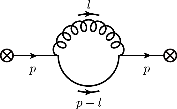
We show schematically the assignment of momenta in Fig. 1. The total momentum of the final state is $p$ with $p_{-}=Q$ for the jet in the $n$ direction. And $p^{2}$ is the invariant-mass squared of the collinear jet. In order to obtain the scattering cross section, we cut the diagram in all possible ways and add their contributions. When we cut the loop, there are two final-state particles with the momenta $l$ (for a gluon) and $p-l$ (for a quark or an antiquark). If we cut a single line, it gives virtual corrections. The collinear gluon momentum $l^{\mu}$ in the $n$ direction scales as

$$l^{\mu}=(l_{-},l_{\perp},l_{+})\sim Q(1,\lambda,\lambda^{2}),$$

(24)

where $Q=p_{-}$ is the largest momentum component of the collinear jet.

A cone-type algorithm collects all the particles within a fixed cone of radius $R$, which determines the jet size. The jet axis is determined, for example, by a thrust axis. There are many issues on how to construct cone jets including infrared safety. But if we confine ourselves to the jets at the next-to-leading order, there are at most two particles in a jet and all the cone-type algorithms are reduced to a generic cone-type algorithm. For collinear particles, if two particles are in the cone of radius $R$, that is, if $\theta_{q}<R$, and $\theta_{g}<R$, where $\theta_{q}$ and $\theta_{g}$ are the angles of the quark and the gluon with respect to the jet axis, they form a jet. In terms of the momenta shown in Fig. 1, this corresponds to the cone algorithm for the collinear particles:

$$\Theta_{\mathrm{cone}}=\Theta\Bigl(t^{2}>\frac{l_{+}}{l_{-}}\Bigr)\Theta\Bigl(t^{2}>\frac{s/Q-l_{+}}{Q-l_{-}}\Bigr),$$

(25)

where $t=\tan R/2$ with the jet cone radius $R$. Each term in $\Theta_{\mathrm{cone}}$ represents $\theta_{g}<R$ and $\theta_{q}<R$ respectively.

In the SW jet algorithm, a two-jet event is defined as the one in which the total energy $Q$ except the fraction $\beta$ is deposited in two jet cones with half angle $\delta$. This algorithm can be split into a collinear part and a soft part, according to which the factorized result is written in Eq. (17). For the collinear part, the two particles are energetic and, if we let $\theta$ be the angle between the two particles, the jet algorithm states that $\theta<2\delta$, which is equivalent to $1-\cos\theta<1-\cos 2\delta$ for $0<\theta<\pi$. For the jet in the $n$-direction, combining the on-shll conditions $l^{2}=0$, $(p-l)^{2}=0$, and using the hierarchy of lightcone momenta, this corresponds to

$$\Theta_{\mathrm{SW}}=\Theta\Bigl(t^{2}>\frac{Q^{2}l_{+}}{l_{-}(Q-l_{-})^{2}}\Bigr),$$

(26)

with $t=\delta$.

We will use $t$ both for the cone radius ($t=\tan R/2$), and the angle ($t=\delta$). So far, the cone size is independent of the power counting of momenta in SCET. For example, if $R=\pi$ for the entire hemisphere, $t=\tan R/2\sim\mathcal{O}(1)$. However, if $t$ is too small, the constraint of the jet algorithm does not work. The size of the parameters $t$ and $\beta$, related to the jet algorithm, should be determined by the physics we consider. As can be seen in Eq. (26), with the fact that the collinear momentum scales as $(l_{-},l_{\perp},l_{+})\sim Q(1,\lambda,\lambda^{2})$, the power counting $t^{2}\sim\lambda^{2}$ produces a nontrivial jet algorithm. Therefore here we consider the case with $t\sim\lambda$, and $t$ can be used interchangeably with $\tan R/2$ or $\delta$. For the jet in the $\overline{n}$ direction, the corresponding condition is given by switching $l_{+}$ and $l_{-}$.

To avoid double counting, the zero-bin contribution should be considered [20], where the collinear momentum $l^{\mu}$ approaches the soft-momentum limit

$$l^{\mu}=(l_{+},l_{\perp},l_{-})\sim Q(\lambda^{2},\lambda^{2},\lambda^{2}).$$

(27)

The corresponding zero-bin phase space is expressed as

$$\Theta^{(0)}=\Theta\Bigl(t^{2}>\frac{l_{+}}{l_{-}}\Bigr).$$

(28)

This is common to the cone-type and the SW jet algorithms. The phase spaces given by the jet algorithms are shown in Fig. 2. Fig. 2 (a) is the phase space available for the naive collinear contribution in the cone-type jet algorithm, Fig. 2 (b) is the phase space available for the SW jet algorithm, and Fig. 2 (c) is the phase space for the zero-bin contribution for both jet algorithms.

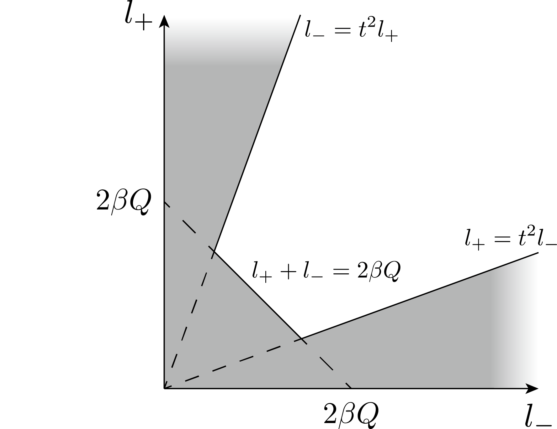
We use the same constraints for soft particles in both algorithms. That is, when a soft gluon is inside the cone either in the $n$ or $\overline{n}$ directions, it is included in the jet. An additional constraint on the soft function is about a jet veto. If a soft particle is outside the jet, the energy of the soft gluon is less than $\beta$. The soft momentum scales as $Q\lambda^{2}$, and the nontrivial constraint from the jet veto occurs when $\beta\sim\lambda^{2}$. From now on, we fix the power counting on the parameters in the jet algorithm as $t\sim\lambda$ and $\beta\sim\lambda^{2}$.

Then the constraint on the soft function from the jet algorithm can be expressed as

$$\Theta_{\mathrm{soft}}=\left\{\begin{array}[]{ll}\displaystyle\Theta\Bigl(t^{2}>\frac{l_{+}}{l_{-}}\Bigr),&(n\ \mathrm{jet}),\\ \displaystyle\Theta\Bigl(t^{2}>\frac{l_{-}}{l_{+}}\Bigr),&(\overline{n}\ \mathrm{jet}),\\ \Theta(l_{+}+l_{-}<2\beta Q),&(\mathrm{outside}\ \mathrm{the\ jet}).\end{array}\right.$$

(29)

Fig. 3 shows the phase space for the soft function. The shaded area is allowed by the jet algorithm in Eq. (29)

Note that we include the constraint from the jet veto in the jet algorithm of the soft function, not in the collinear function. This is obvious from the power counting since $\beta\sim\lambda^{2}$ and $l_{+}+l_{-}\sim Q$ for the collinear gluon, hence there is no veto needed for the collinear particles. Instead the zero-bin subtraction eliminates the soft limit in the collinear jet function. However, in Ref. [13], the author considered only the jet function with the same power counting on $t$ and $\beta$, but this jet veto was also included in the jet function. This seems to be a different definition of the jet function, compared to ours. But the jet function in Ref. [13] does not depend on $\beta$ after the zero-bin subtraction. That is, the inclusion of a jet veto in the jet function does not alter the result. However, we stress that our definition of the jet algorithm strictly respects the specified power counting of the parameters.

A question arises if the cone-type and the SW jet algorithms can also be employed at hadron colliders. The main difference between $e^{+}e^{-}$ annihilation and $pp$ scattering is that the center of energy is fixed in $e^{+}e^{-}$ annihilation, while it is not fixed in $pp$ scattering. And the center-of-energy frames at the partonic level in $pp$ scattering have a boost invariance along the beam direction. Therefore the jet algorithm in $pp$ scattering should be defined in a boost-invariant way, for example, in terms of the rapidity and the azimuthal angle. The cone-type algorithm can be employed in $pp$ scattering, and the method of defining the jet axis should be employed. The SW jet algorithm seems to be specific to $e^{+}e^{-}$ annihilation. However, at the next-to-leading order in which there are three final-state particles, the inclusive $k_{T}$ algorithms ($k_{T}$, Cambridge/Aachen, and anti-$k_{T}$) reduce to the same constraint as the SW jet algorithm, and can be used in hadron collisions.

The unintegrated jet function $J_{n,\Theta}(p^{2},\mu)$ in the $n$ direction is defined as

$$\sum_{X_{n}}\langle 0|\chi_{n}^{\alpha}|X_{n}\rangle\Theta_{J}\langle X_{n}|\overline{\chi}_{n}^{\beta}|0\rangle=\int\frac{d^{4}p_{X_{n}}}{(2\pi)^{3}}\frac{\hbox{$/$}\kern-5.50117pt\hbox{$n$}}{2}\overline{n}\cdot p_{X_{n}}J_{n,\Theta}(p_{X_{n}}^{2},\mu)\delta^{\alpha\beta},$$

(30)

where $\Theta_{J}$ is the jet algorithm. The integrated jet function $\mathcal{J}_{n,\Theta}(\mu)$ is defined as

$$\mathcal{J}_{n,\Theta}(\mu)=\int dp^{2}J_{n,\Theta}(p^{2},\mu),$$

(31)

where $p^{2}$ is the invariant mass squared of the collinear jet. The unintegrated jet function is the collinear jet function with $p^{2}$ fixed, and it is expressed in terms of distribution functions. When integrated over $p^{2}$, the integrated jet function is obtained. Eq. (31) should hold to all orders in $\alpha_{s}$. But in current literature, there is some confusion between the integrated jet function, which is obtained by integrating the unintegrated jet function, and the inclusive jet function in which there is no jet algorithm involved.

In a different context in Ref. [11], the unmeasured jet function (which is the same as the integrated jet function in our case) is not obtained from the measured jet function (which corresponds to the unintegrated jet function, but different) by integrating with respect to the thrust. The authors claim that the small parameter in power counting is different. That is, in a measured jet sector the small parameter is $\sqrt{\tau_{a}}\sim\lambda$, while $R\sim\lambda^{0}$. Indeed different power counting yields different answers, but as far as the total jet cross section is concerned, the result through the paths from the integrated jet functions, and from the measured jet functions is the same. The relation between these two approaches and the physics behind them will be clarified in Section VIII.

In Sections IV and V, we explicitly compute the integrated and the unintegrated jet functions separately. The difference lies in the different order of integration of the delta functions, but there are subtleties which arise in the detailed calculations. What we also focus on is whether the factorized parts, the jet function and the soft function, are infrared finite themselves. If they contain infrared divergences though the sum of the jet and the soft functions do not, the factorized result is not physically meaningful. In order to show the IR safety explicitly, we employ the dimensional regularization with $D=4-2\epsilon$ and the $\overline{\mathrm{MS}}$ scheme, and regulate both the UV and the IR divergences. In the $\overline{\mathrm{MS}}$ scheme, we put $4\pi\mu_{\overline{\mathrm{MS}}}^{2}=\mu^{2}e^{\gamma_{\mathrm{E}}}$.

We can also employ the dimensional regularization for the UV divergence and the rapidity regulator only in the collinear Wilson line [21, 22] to regulate the rapidity divergence as

$$W_{n}=\sum_{\mathrm{perm}}\exp\Bigl[-\frac{g}{\overline{n}\cdot\mathcal{P}+\Delta+i0}\overline{n}\cdot A_{n}\Bigr].$$

(32)

The final collinear results with the zero-bin subtraction are independent of the regulator $\Delta$ though it appears in individual diagrams, and the result is the same as that with pure dimensional regularization. We present the result for the integrated jet function in the SW jet algorithm in Appendix for completeness.

The Feynman diagrams for the jet function, say, in the $n$ direction, are shown in Fig. 4. The dashed line represents the cut, therefore Fig. 4 (a) is the virtual correction, while Fig. 4 (b) and (c) are the contributions from the real gluon emission. The mirror images of (a) and (b) are omitted in Fig. 4, but they are included in the computation. And we also include the wave function renormalization and the residue from the self-energy diagram for the quark. Each diagram is accompanied by the corresponding zero-bin contribution, which should be subtracted to obtain the collinear jet function.