Another look in the Analysis of Cooperative Spectrum Sensing over Nakagami- Fading Channels
Abstract
Modeling and analysis of cooperative spectrum sensing is an important aspect in cognitive radio systems. In this paper, the problem of energy detection (ED) of an unknown signal over Nakagami- fading is revisited. Specifically, an analytical expression for the local probability of detection is derived, while using the approach of ED at the individual secondary user (SU), a new fusion rule, based on the likelihood ratio test, is presented. The channels between the primary user to SUs and SUs to fusion center are considered to be independent Nakagami-. The proposed fusion rule uses the channel statistics, instead of the instantaneous channel state information, and is based on the Neyman-Pearson criteria. Closed-form solutions for the system-level probability of detection and probability of false alarm are also derived. Furthermore, a closed-form expression for the optimal number of cooperative SUs, needed to minimize the total error rate, is presented. The usefulness of factor graph and sum-product-algorithm models for computing likelihoods, is also discussed to highlight its advantage, in terms of computational cost. The performance of the proposed schemes have been evaluated both by analysis and simulations. Results show that the proposed rules perform well over a wide range of the signal-to-noise ratio.
Index Terms:
Cognitive radio, spectrum sensing, binary hypothesis testing, likelihood ratio, factor graph, sum-product-algorithm.I Introduction
It is well-known that most of the licensed spectrum is not fully utilized all the time [1], when fixed spectrum allocation is used. Moreover, the rapid deployment of new wireless devices and applications with growing data rates creates a spectrum scarcity problem. Cognitive radio networks (CRN) [2] is an emerging solution to the problem of inefficient use of allocated licensed spectrum. In this approach, the secondary users (SUs) or cognitive radios (CR)s are allowed to sense the spectrum dynamically, identifing the spectrum holes i.e. in the absence of a primary user (PU) - in the target spectrum pool and opportunistically utilize it.
I-A Motivation and Literature
Spectrum sensing is the first critical step of the CR cycle [2] in order to dynamically utilize the unused spectrum. Sensing techniques can be classified as, a) Local Sensing: Each SU individually and/or independently detects spectrum holes. Although this kind of sensing is sensitive to fading, shadowing, and model uncertainty, it has a simple implementation. A brief survey of different spectrum sensing techniques was presented in [3]. Furthermore, it is shown in [4] that the energy detection (ED) is optimal for detecting zero-mean constellation signals, if no prior knowledge about PU’s signal is available at the SU, except of the received signal power. Note, that ED is also popular due to the simplicity of its implementation [5]. b) Cooperative Sensing: Information from multiple SUs are jointly used to detect spectrum holes, and to mitigate multipath, shadowing etc., by exploiting the spatial diversity among CRs. It enhances accuracy, reliability, and performance of sensing at the cost of complexity. Moreover, cooperative sensing is most effective, when collaborating CRs observe independent fading or shadowing [6, 5, 7, 8, 9, 10, 11].
Cooperative sensing may be further viewed as distributed detection problem, with the central coordinator to be the fusion center (FC). This is also known as centralized cooperative spectrum sensing (CCSS) and is investigated in this paper. A detailed survey on the distributed detection was presented in [12]. In this kind of detection, likelihood ratio test (LRT) rule is known to be optimal. However, a global optimal solution with coupled local best rules is known to be NP-hard and not available in closed-form [13]. Moreover, it was proved that ED is optimal for single-sensor detection [14], while identical decision rule is asymptotically optimal for global decision in a large network [13]. LRT is implemented using either the Neyman-Pearson (N-P) criterion (maximization of probability of detection subject to a constraint on probability of false alarm) or the Bayes criterion (minimization of error) [15].
Well-known sub-optimal fusion rules for ideal SU-FC (reporting) channels are: AND, OR, and VOTING [12]. Other sub-optimal decision fusion rules over noisy channels are Chair-Varshney fusion for the high signal-to-noise ratio (SNR), equal gain combining (EGC) for low SNR, and maximum ratio combining (MRC) for medium SNR [16]. Recently, suboptimal fusion rules, known as optimal linear cooperation strategy for additive white Gaussian noise (AWGN) and linear-quadratic (LQ) strategy for ideal reporting channels have been discussed in [17] and [18], respectively. Furthermore, in [14, 19], the authors used a probabilistic graphical approach to model the optimal LRT based fusion for cooperative spectrum sensing. Other sensing algorithms for PU detection, such as optimum matched filtering [20], eigenvalue based detection [21], cyclostationary feature detection [22], generalized likelihood ratio test (GLRT) based sensing [23, 24], were also reported in literature.
Good message-passing algorithms, like Pearl’s belief-propagation (BP) algorithm and sum-product algorithm (SPA) [25] over suitable graphical models, have been successfully employed for solving inference problems in various aplications, e.g. data mining, computational biology, statistical signal processing, and wireless communications. This approach provides exact solutions for acyclic graphs, while exhibiting a low computational complexity, compared to explicit methods [26]. Moreover, BP/SPA is inherently suitable for distributed implementation [25]. Therefore, it becomes a practical and powerful tool to solve distributed inference problems, such as cooperative spectrum sensing in CRNs [19, 14].
In the spectrum sensing literature, previous studies assume approximate channel statistics [18, 27, 21] or known [17, 7, 8] or estimated [23, 24], instantaneous channel state information (CSI). The effects of different signal models with known CSI on sensing have also been investigated in [28, 7]. Furthermore, the problem of energy detection of an unknown signal over Nakagami- fading was addressed in a few papers [29, 30], but, the results were presented only for high SNRs. Regarding the decision fusion most of the works consider non-ideal sensing channels with ideal [12, 31] or binary symmetric (BSC)/AWGN reporting channels [17, 19, 32]. Optimization of the CCSS scheme over Rayleigh fading and ideal reporting channels, was also addressed in [31]. Furthermore, decision fusion over non-ideal reporting channels was introduced by [16], in the context of wireless sensor networks (WSN). However, multipath fading on sensing and reporting channels is common in a CRN and limits the performance of CCSS. However, none of the above works consider multipath fading on both PU-SUs and SUs-FC links, simultaneously.
Nakagami-, is a general fading model [33], which often gives the best fit for land and indoor mobile applications [34, 35, 36, 37]. However, cooperative spectrum sensing, in the presence of Nakagami- fading with channel statistics, is relatively less investigated. Moreover, SUs may be mobile in many applications, like object tracking, environment, habitat management etc., where the channel estimation is costly. Therefore, spectrum sensing over Nakagami- fading for a wide range of SNR and LRT based decision fusion without knowledge of instantaneous CSI, is useful for the system design. Moreover, in a large CRN it also involves conditional and unconditional independence on large number of random variables (RVs) and thus it leads to an increase of the overall system complexity. Hence, inference over graph with message passing is a good approach for this problem [14, 19].
I-B Contribution
In this work, we study the performance of CCSS systems, by assuming that both PU-SU and SU-FC channels are Nakagami- and independent accross the SUs. The LRT statistics is computed through message passing over the representative NFG, in order to reduce the computation complexity. Specifically, the main contributions of this paper are as follows.
- •
Derivation of an LR based fusion rule without knowledge of the instantaneous CSI. Closed-form expressions for the system level probabilities of detection, , miss, , and false alarm, , are also derived. Furthermore, we present an alternate expression for the local probability of energy detection over Nakagami- fading.
- •
Determination of the optimal number of cooperating SUs, needed to minimize the total error rate, , as a function of the SNR and the total number of SUs.
- •
Modeling of CCSS using NFG and SPA in order to analyse the computation time complexity, compared with explicit method.
I-C Structure
The rest of this paper is organized as follows. Section II refers to NFG and SPA, while Section III represents the system model, the assumptions used, and the problem formulation. Expressions for local probalilities of detection and false alarm are presented in Section IV, while the LRT-based fusion rule with NFG-SPA based model, closed-form analysis of system-level performance metrics and optimization of the CRN, are presented in Section V. Simulation results are reported in Section VI, and the complexity analysis and advantages of NFG-SPA settings are discussed in Section VII. Finally, Section VIII concludes the paper and propose some future research directions.
I-D Notations
Throughout this paper, denotes the total number of SUs present in the CRN, denotes the total number of (complex) signal samples available for detection, also known as time-bandwidth product. We use to denote the set of RVs . Here, denotes statistical expectation, denotes modulus of , denotes probability density function (pdf) and denotes cumulative distribution function (cdf) of . , , and denote Nakagami- distribution with fading severity parameter , complex Gaussian, and real Gaussian distribution, respectively.
II Factor Graph, Sum-Product Algorithm (SPA)
Probabilistic graphical model (PGM) [38] is an effective way to represent the probabilistic dependencies between RVs. Well-known graphical models are Bayesian network (BN), Markov random field (MRF), Tanner graph (TG), junction tree (JT), and factor graph (FG) [38]. Among those, FGs are more general, since any BN, MRF or TG can be transformed as FG, with no increase in its representation size [25]. Throughout the present work, we consider a version of FG, called normal factor graph (NFG) [26], as the PGM. The primary goal of FG-SPA based modeling of CCSS is to reduce computational complexity.
II-A Factor Graph
Factor graph is a standard bipartite graphical representation of a mathematical relation between variables and local functions. There are two types of factor graphs [26]: conventional and normal (Forney-style) factor graph (NFG). In an NFG, functions or factors are represented by nodes and variables are represented by edges.
Example: Consider a joint probability mass (density) function of variables as .
Suppose, the function is factorized as
| (1) |
where is a normalization factor. Alternatively, it can be represented through a graph with function nodes and variable edges. We consider the factorization with and , where one variable is involved in more than two factors. Then,
| (2) |

Fig.1 depicts an example of (2) as a normal factor graph. We summarize the construction of NFG as follows:
- •
Equality node, , indicates variables corresponding to more than two functions i.e. the node with degree, .
- •
Computation of marginal can be performed in an efficient and automated way by using SPA on factor graph.
- •
A function can have many factorizations; therefore, it can have many factor graphs. As long as the graphs have no cycles, the same marginal will be computed for all.
II-B Sum-Product Algorithm and Message Passing
Sum-product algorithm (SPA), also known as message-passing or belief-propagation (BP) algorithm, can often be applied successfully in situations, where exact solutions to the marginalize product-of-function (MPF) problems become computationally intensive [25, 38]. SPA operates over an NFG associated with the global function and computes various marginal probabilities by approximating through beliefs. Let us define the message from function node to variable edge as . The message from variable edge to function node is denoted by , where and are the set of neighboring functions of and the set of variables involved in function , respectively. Message from edge to node is computed as
| (3) |
and message from node to edge is computed as
| (4) |
where denotes all the nodes/edges that are neighbors of edge/node except for node/edge . In SPA, sum is due to summation and product is due to product operation in (4). In case of continuous variables, summation operation is replaced by integration. The proportionality sign in (3) and (4) is used to indicate a normalization factor, such that the distribution sums/integrates to one. Final marginal for any variable is calculated as belief i.e. the product of all incomming mesages as
III System Model for CCSS over Fading Channels
The block diagram of CCSS system is shown in Fig. 2. It consists of one PU, number of SUs, and one FC. All SUs are independently sensing the PU and then sending their local decisions to FC. Final decision is taken by the FC.

III-A Assumptions
Throughout this paper, Nakagami- fading is used to model rapid fluctuations of the amplitudes of a radio signal, and it is assumed that the average sensing duration is much shorter than the average busy-to-idle and idle-to-busy state transition periods of PU [31]. Transmit power of PU is assumed to remain constant over a typical sensing period and a prior probability of PU’s traffic is unavailable at each SU.
Furthermore, it is assumed that all SUs stay silent during the sensing interval, such that the spectral power remaining in the targeted band is transmitted only by the PU. Next, it is considered that all SUs use same transmit power relative to the PU (as in the interweave Dynamic Spectrum Access (DSA) model [39]) and each SU makes a binary local decision (hard-sensing) using ED [6]. At FC, the final decision () is taken when local decisions from all SUs are arrived. We formulate our problem by assuming that all sensing and reporting channels are time-invariant (during the sensing process), frequency-flat fading and statistically independent, across different SUs.
III-B Problem Formulation
Suppose that all SUs monitor the same frequency with the PU (Fig. 2). Spectrum sensing at the -th SU can be formulated as a binary hypothesis testing problem [15]. The received signal samples at for the two hypotheses can be modeled as
| (5) |
where , , is the sample of AWGN, and represents the signal sample, received from the primary user if active. The signal is modeled as RV with average power of , which includes the channel gain. In practice, and are independent.
Classically, the received primary signal samples at are assumed (reasonable approximation for unknown PU signals over fading; [23, 24, 14]) to be independent and identically distributed (i.i.d.) complex Gaussian RVs with zero mean and variance, . This implies that the magnitude of the complex envelope is Rayleigh distributed. However, in practice, the received signal at each is composed of a large number of resolved multipath components. Therefore, the magnitude of the envelope is the norm of an -dimensional complex vector, where is the fading parameter of the Nakagami- distribution [40]. Therefore, , and the average power of the received primary signal can also be written as [40]. The average received SNR of the link, measured at , is defined as
| (6) |
At , the ED computes the energy of the received signal over samples. The computed energy is compared with the threshold , which is determined from a given local probability of false alarm, and the binary local decision is generated, where and denote absence and presence of the PU, respectively. Therefore, the test statistic at becomes
| (7) |
Each decision, , is transmitted to the FC over an independent, frequency-flat fading channel. The signal received at the FC from is
| (8) |
where is the observation noise and is the secondary signal, over the link. Similarly, we assume , where the average power of the signal is . In practice, and are independent and the noise samples at FC and SUs are also independent across different links. The average received SNR for link is defined as .
The vector of received signal at the FC from all SUs is denoted by . For any the binary hypothesis problem at FC is
| (9) |
where and are the distributions of in absence () and presence () of the PU, respectively. Final decision () is derived at the FC by LRT using these two distributions.
We assume that SUs use the spectrum, whenever they detect a spectral hole (white space). The constraint in the system model is the probability of erroneous decision about the presence of the PU. Hence, for efficient utilization of spectrum, according to Neyman-Pearson criteria [15], the system designer needs to minimize the probability of miss or maximize the probability of detection, subject to the constraint that the probability of false alarm satisfies a minimum requirement.
IV Local Performance Analysis
This section presents the local performance analysis (probabilities of detection and false alarm at ) for the system model defined in section-III.B. Throughout the analysis, the variable is used as for notational simplicity.
IV-A Analysis Under the Hypothesis
Under , the received signal contains only noise and thus, . As the number of complex samples is considered as sensing period, the pdf of under follows Chi-square distribution with degrees of freedom [41]. In this case, the probability of false alarm at is obtained as [29]
| (10) |
where , , and are the lower incomplete gamma, upper incomplete gamma, and complete gamma functions, respectively [41]. Assuming that the noise variance is perfectly known, the local threshold is obtained for a given as
| (11) |
IV-B Analysis Under the Hypothesis
Under the hypothesis , the received signal contains both PU signal and noise. Therefore, the distribution of the test statistic depends on distribution of the envelope of the signal (i.e. ), which further depends on . The unconditional pdf of under is obtained using Bayesian approach, i.e. marginalizing the conditional pdf of over . Here, is Nakagami- distributed [33] and is defined as
| (12) |
The pdf of under is obtained as
| (13) |
where , , , , and is the confluent hyper-geometric function [41, (13.1.2)].
As, and is complex, has degrees of freedom. After a transformation of the variables in (13) we get the pdf of under as
| (14) |
Integrating (14) using Laguerre polynomials [42], [43, (6.9.2.36)], and after some algebra [41, (6.5.12)], the local probability of detection can be written as
| (15) |
In (15), is the hypergeometric function of two variables [41]. The steps for (14)-(15) are given in Appendix B. Note that Eq. (15) is more general (as it holds ) than [29, (7)], which is restricted to integer . Moreover, Eqs. (15) and [29, (7)] can be implemented via the MATHEMATICA software, which requires truncation of infinite series and computation of error bounds [44, 30]. However, a general closed-form expression of is intractable, due to the presence of , , and in (14), simultaneously [41]. Therefore, it is interesting to find for specific values of .
Case-I:
For , (13) is simplified as
| (16) |
where and is the well-known Gaussian -function [41]. For the derivation of (16) see Appendix C. Setting in (14) and using [41, (6.5.12)] we obtain
| (17) |
where . The cdf is obtained by integrating (17) over using [45, (1.2.2.1)]. Hence, the probability of detection at can be written as
| (18) |
Case-II:
Similarly, for , (14) can be written as
| (19) |
where . With the help of Appendix D, the probability of detection can be expressed as
| (20) |
Similarly, using other values of in (14) and integrating over , corresponding ’s can be obtained. For example, an expression for , when , is presented in Appendix F.
IV-C Approximate Complex Representation of the Nakagami- Envelope
In [47], it is shown that the exact distributions of real and imaginary parts of the complex signal for Nakagami- envelope are non-Gaussian. As a special case, either the in-phase or quadrature signal may be assumed as zero-mean Gaussian, while the other part will be non-Gaussian [47]. In [46], the distributions of in-phase and quadrature parts of a signal having Nakagami- fading envelope, are derived for both and . However, at high SNRs, the proposed model of [46] closely approximates the distributions of real and immaginary parts of signals with Rician [46, (59)] for and Hoyt [46, (61)], for fading envelopes. These approximations are considered here for simplicity. However, for , can be assumed as for all SNRs [23, 24, 14, 19]. Therefore, with the help of [46], the complex signals over Nakagami- fading can be written as
| (21) |
where , and , , and . is defined in [46, (39)]. PU is active under and the distribution of the decision statistic is obtained from that of the signal. At high SNR, the distribution of can be approximated according to (21) for different range of , as in [46]. Thus, the associated probabilities of detection at for different values of are obtained as follows
IV-D Comparisons of the Two Models


Figs. 3 and 4 plot receiver operating characteristic (ROC), i.e. vs curves for different values of SNR dB, dB, and dB, over Nakagami- fading with , and , respectively.
It is observed from Fig. 3 that both analytical models for perfectly match with simulations for all SNRs. Further Fig. 4 shows that, for , at very low SNR none of the models matches with simulations, but, it becomes closer to the proposed model in (20). However, at moderate SNRs ( dB to dB) the simulations match with the results of the proposed approaches, while it matches perfectly at high SNR ( dB). Therefore, we can say that for , the analysis based on the complex signal model [46] is only suitable for high SNRs. However, (22) is reasonable and also validates the well-known approximation of for [19, 23, 24]. Note that, the analytical models proposed in this paper suit well over a wide range of SNR for . A similar comparative study can be presented for . It can also be proved that the proposed model in (61) suits better than the complex one in (22) over a wide range of SNR. In this paper, we drop the figure for due to space limitations.
Fig. 5 plots complementary ROC i.e. vs curves for different SNRs ( dB, dB dB) over different fading channels () and compares the proposed model with Digham et. al’s [29]. It is observed that the model proposed in this paper is better than [29] over a wide range of SNR. Hence, we always consider the analytical models of (18), (20), and (60) for further system-level analysis in the next section.
V System-level Performance Analysis
V-A Probability Models of the Detection Problem
The CSS problem, described in Fig. 2, can also be viewed as a system-on-graph (Fig. 6). Thus, we can model the problem as inference over the representative NFG and try to solve it by passing messages over the graph using SPA. This approach can adopt all the unknown parameters, such as signals, channel effects, noise, and complex dependencies in a single framework. It is shown that the FG-SPA approach finds the desired likelihoods in an automated way. Accomplishable reduced complexity is shown in Section-VII.
As explained above, the goal is to find the likelihood functions, and , in order to compute the LRT statistic and thus, to solve the distributed detection problem. These likelihoods can be obtained by marginalizing the joint probability distribution of interest over all unknown variables. Thus the detection problem is mapped to a Bayesian inference one, in order to find the likelihoods through message passing via SPA over the representative NFG. The joint probability distribution represents the CCSS model of Fig. 2. Likelihood functions, represented by for , can be evaluated as
| (23) |
where is the joint distribution of interest. This can be further factorized as
| (24) |
The last line in (24) holds because the channels are independent accross the SUs. Fig. 6 represents the NFG for the joint distribution of interest . Each branch represents the PU-SU-FC path of Fig. 2. The equality node, , indicates that variable is associated with more than two functions i.e. with all . It computes likelihoods from the joint distribution by employing hard decisions at SUs. The graph has no cycle, as all PU-SU-FC channels are statistically independent. Therefore, SPA can compute the exact marginals over the graph.
V-B Computation of Messages in NFG-SPA Settings
In NFG, probability functions are represented by nodes and variables are represented by associated edges. The desired likelihoods and have to be computed from the graph. By applying the SPA as message computation rule [26], intermediate messages are computed and passed between the nodes of the FG. The message propagation follows a single step of natural scheduling. As the graph has no cycle, the computation of messages starts from the half edge () (edge connected to only one node) and leaf node ( and ) and proceed from node to node. The message () from the leaf node () to the connecting edge () is the marginal value of the function (node) with respect to that variable (edge). For half edge, the message () from the edge to the node is initialized with the value . For intermediate nodes, all incoming messages to that node are computed first and every message is computed only once. The messages are indexed with and are shown in Fig. 6 on the corresponding edges of the graph. Dotted arrows show the flow of messages for computing the marginals. Step-by-step computations are presented in Appendix A.
The marginal of on th branch is computed from the final messages of interest similarly as [19, (21)]
| (25) |
where
| (26) |
is obtained by marginalizing over , and is local threshold at -th SU.
The final message on each branch is computed as the product of messages from node to edge and from edge to node . The desired likelihood functions for cooperative sensing are obtained from the marginal distribution of and computed as the accumulated final message (product over all branches) over all edges for from (25) as
| (27) |
Likelihoods are computed in automated way using NFG-SPA.
V-C Analysis of Decision Fusion at FC
LRT based decision fusion is performed at the FC. It requires likelihoods under and for each received signal . Using (25), the likelihood under can be viewed as the message under and can be written as [19, (23)]
| (28) |
Similarly, the likelihood under can be written as
| (29) |
As the observations are independent, the LRT for choosing in N-P method can be written with help of (27) as
| (30) |
where is the threshold at FC. In N-P settings, this is obtained by solving
for a constraint on probability of false alarm at FC.
According to (8), and the envelope of the received signal at FC over link is Nakagami- distributed i.e. . In general, follows (13) by replacing , and with , and , respectively. For , as follows (16), the LRT statistic (using Appendix E) can be written as
| (31) |
Similarly, for , the LRT statistic (using Appendix E) is given by
| (32) |
where , , , , , and is obtained from (10). The ’s are obtained from (18) and (20) for and , respectively. Similarly, other likelihood ratios may be obtained by substituting corresponding values of in (30) with associated ’s. The LRT statistic for is derived in Appendix F.
According to this approach, local thresholds are derived, based on the probability of false alarm, and therefore, CSI is not needed at each SU. However, local probabilities of detection and final LRT statistics, i.e. values, depend on channel statistics instead of instantaneous CSI. Moreover, system-level thresholds for LRT at FC are selected based on the values. Therefore, we can state that, for the overall system design, the proposed fusion rule requires the knowledge of channel statistics, i.e. average SNRs and instead of the instantaneous CSI.
V-D Closed-form Analysis
Eqs. (31) and (32) are LR based fusion rules, but, the derivation of closed-form expressions for and from them, seems to be a hard task. However, LR based optimum fusion rule can be approximated as Chair-Varshney one [13], under the assumption of high SNR and identical detectors (i.e. , ) [16]. It is already assumed that ’s are statistically i.i.d. for large number of SUs. To derive the closed-form expressions for and , we also define as the number of SUs for which and the number of SUs for which . Hence, the log-likelihood-ratio (LLR) from (30) can be written in terms of and
| (33) |
Therefore, is binomial distributed, where the probability of success is defined as . Let us denote, and are the probabilities of success under and , respectively. Then, the system-level detection performance, i.e. , and can be computed using the binomial distribution. Associated closed-form solutions are
| (34) |
| (35) |
where takes values from to . For , and can be evaluated as (see Appendix E for the derivation)
| (36) |
Similarly, and are obtained for other values of with associated (see Appendix E and F). Hence, we state that N-P test is equivalent to J-out-of-K rule when
- •
All PU-SU-FC channels are statistically independent.
- •
All SU’s are employing identical decision rules and transmitting hard local decisions to FC.
V-E Optimization of Cooperative Spectrum Sensing
In general, when increases, also increases and as a result decreases. However, an effective system design should always minimize the total error rate, . An optimal voting rule that minimizes Bayes risk function has been addressed in [13, (pp. 94)]. Minimization of over ideal SU-FC channels using some linear approximation has also been reported in [31]. Next, we investigate the optimal number, , of SUs required to minimize the total error rate over non-ideal SU-FC channels.
Let, be the number of SUs required to achieve certain values of and . From (34) and (35), let us define a function . Therefore,
| (37) |

From the properties of ROC curve [15], it is known that . Then, from (36) and (58) for and , respectively, holds that . Under this condition, it is evident from (37) that minimization of is equivalent to the minimization of . Now, when is increased by 1, it holds that
| (38) |
From (38), if,
| or, | ||||
| or, | (39) |
Similarly, when is decreased by 1,
| (40) |
From (40), if
| (42) |
where
and , are given by (36) or (58). Therefore, depends on , , and , subject to the constraint . These probabilities of success under and further depend on the average SNRs of SU-FC channels, local thresholds (), noise variance () of individual ’s, and average SNRs of PU-SU channels. Hence, it is observed that the optimal number of SU () depends on , , and average SNRs and . Moreover, it is concluded that a fast spectrum sensing algorithm can be executed by considering only SUs instead of all in a CRN, with statistically independent channels.
Fig. 7 plots the number of cooperating SUs vs for different values of and different channel conditions. The figure shows that, for a fixed average SNR of dB over SU-FC channels, the optimal number of cooperating SUs increases from to , while the total number of SUs increases from 15 to 20, respectively. It can also be observed that as increases, of corresponding decreases. However, to achieve a given (say, 0.63) with fixed , the required number of cooperating SUs () increases from 10 to 12, as the average SNR decreases from dB to dB. It infers that, for a fixed values of , the value of increases to achieve a given (bounded) , as SNR decreases. Hence, we can say that there exist an optimal number of cooperating SUs for different and different SNRs, subject to minimization of .
VI Simulations and Discussions
In this section, simulation results are presented to evaluate the proposed CCSS scheme. The parameters used in the simulations are: , and , and number of Monte Carlo iterations . Independent, frequency-flat, Nakagami- fading with and , and , are considered. In the following, ED threshold () at , , are obtained from (11), to maintain a target local probability of false alarm . However, each has different probabilities of detection () based on the different valuse of (e.g. (18), (20) for , respectively). The system-level performance is quantified by the ROC. The average SNRs of sensing and reporting channels are defined as and , , respectively.
Fig. 8 describes the ROC curves at different LRT threshold levels, for different fusion statistics of the CCSS. It is assumed that, dB and dB, , and . It can be seen from Fig. 8 that the performance of the LRT based proposed fusion rule is better than the two suboptimal schemes, e.g. EGC and MRC [16], when . Fig. 8 also depicts that the ROC curve improves as increases for all channels, since the effect of fading decreases.
A more practical heterogeneous scenario with 10 SUs is also considered in Fig. 8. It is assumed that in the first six PU-SU-FC channels, and for the rest four channels, . It is shown that ROC performance improves for the heterogeneous case, when compared with that of , because of the SU’s spatial diversity (i.e. different fading severity parameters).

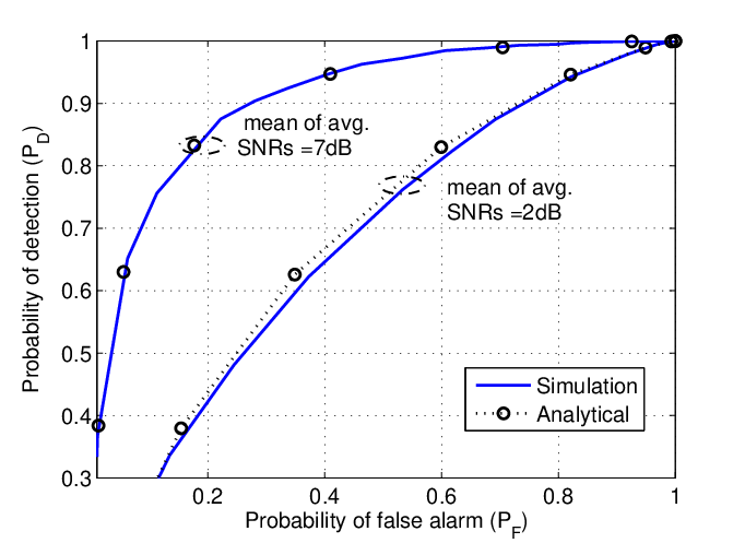
Fig. 9 represents the ROC curves at FC of the LRT based proposed fusion rule, with , , and . We consider single set of average SNRs for PU-SU links as dB, where the mean of all the average channel SNRs for the PU-SU links is dB. However, the two sets (low and high) of average SNRs for SU-FC links have been considered as dB and dB. Here, the means of all the average channel SNRs for SU-FC links are dB and dB, respectively. The system-level analytical results and Monte Carlo simulations are obtained from (34)-(35) and (31), respectively. As expected, ROC performance increases as average SNRs of SU-FC channels increase.
For better clarity, in Fig. 10, the local and system-level probabilities of detection are plotted as a function of the mean of the average SNRs of all the PU-SU channels. The cases of with , , and , are considered. Here, SU-FC channels have mean of all the average SNRs dB and that for PU-SU links are varying from dB to dB. Note that there are significant variations for average PU-SU channel SNRs. In Fig. 10, the performances of both cooperative and non-cooperative sensing schemes are presented for different values. It shows that cooperation among SUs significantly improves the probability of detection compared to the non-cooperative case, over a wide range of SNR. It is also observed that for , the coopeative scheme achieves probability of detection at dB of SNR, whereas non-cooperative sensing reaches to the same at higher SNR ( dB). Fig. 10 also shows that the probability of detection increases significantly for all SNRs, as increases from 1 to 2, in both the cases.

Fig. 11 plots ROC curves obtained from (34)-(35) for different values of and with . The case of dB and dB are considered. Here, the mean of the SNRs for PU-SU and SU-FC channels are dB and dB, respectively. For , SNRs are drawn from index 3 to 7 of the above sets (to maintain the same mean for both ). It shows that detection performance increases significantly as the number of cooperating users increases from 5 to 10 for and both. The reason is the accumulation of information from more number of SUs.

VII Complexity Analysis and Advantage of NFG-SPA Based Approach for the Sensing Problem
The usefulness of the NFG-SPA based approach to cooperative spectrum sensing problem can be analyzed via the computational cost to find the marginal likelihoods. A function may be factorized in several ways, resulting in respective FGs. As long as the graphs are acyclic, the same marginals will be computed. The physical meaning of acyclic is that all PU-SU-FC channels are statistically independent. However, in correlated cases it may lead to more complex SPA, due to the presence of cycles in the graph [25].
The complexity of an algorithm is usually measured in terms of its performance as a function of the size of the input. Here, it depends on the number of functions (nodes) and variables (edges) [26]. Let us consider a function with variables that may be factorized (acyclic) in factors. We assume that each variable is defined over the same discrete-sampled values from a continuous domain or domain for discrete RVs. The function is represented by an NFG of nodes. Suppose, among nodes, have degree 1, have degree 2,…, have degree , where is the maximum degree of a node in the graph. For simplicity, we assume that 1 CPU cycle is required for computing message at any node and that time is negligible at any edge. Then the total complexity (in CPU cycles) in the graphical method can be written as [26], , where is the cardinality of the domain of RVs. Following the conventional (explicit) method, it is required to integrate out all other variables which has a complexity equal to . Thus, the NFG-SPA based approach () is computationally more efficient than the explicit method (. In general , hence .
Example: Consider the graph of Fig. 6 with , i.e. the case of and assume . Therefore, the total complexity to find the marginals using the graphical method is
| (43) |
In comparison, the complexity in the numerical method is
| (44) |
It is interesting to note that NFG is computationally more efficient by times than the conventional method.

To understand the advantage of the factor graph for the distributed detection problem addressed in this paper, Fig. 12 plots the computation complexity as a function of the number of RVs involved. The desired likelihood is obtained by marginalizing in (23). Each variable of interest of the function is defined over the same discrete-sampled values from a continuous domain (i.e. uniformly quantized with levels). We consider two cases as , and for . From the previous discussions and Fig. 6, in this case , . The total complexities to find likelihoods in both conventional ((23)) and graphical ((24)) methods are computed as
for , and
for , respectively. Fig. 12 shows that the complexity monotonically increases with the number of RVs involved (i.e. as the system becomes more complex) in both methods. It also shows that complexity increases as the quantization level increases. However, it is interesting to note that the rate of increment in NFG-SPA setting is considerably less than that of the explicit method. It implies that NFG-SPA setting is computationally more efficient (e.g. times for ) than the conventional method (for acyclic FG). Therefore, we can state that for a large network and higher quantization level, graphical method is more effective from an implementation point of view, even for statistically independent channels. Moreover, collaborative spectrum sensing is very effective, when collaborating CRs observe independent fading [5], which results in acyclic FG. Hence, NFG-SPA settings are suitable from implementation perspective.
VIII Conclusions
In this paper the problem of centralized cooperative spectrum sensing over Nakagami- fading in a CRN, was addressed. We have presented a new fusion rule based on LRT, which requires only the statistical characteristics of the wireless channels between PU-SU-FC. It was compared with other suboptimal rules e.g. EGC, MRC and better performance has been observed. Furthermore, we derived a novel expression for the local probability of detection for ED over Nakagami- fading. It is shown that the proposed models perform better, over a wide range of SNR for different values of , compared to the approximate complex signal representations. Closed-form solutions for the system-level probabilities of detection () and false alarm () were derived. Furthermore, an expression for the optimal number of cooperative SUs, needed to minimize the total error rate, is also obtained. It leads to a fast spectrum sensing algorithm, by considering only the optimal number () of cooperative SUs instead of the total one. Furthermore, decision fusion based on SPA over representative factor graphs was used. It was shown that a considerable amount of gain in computational complexity can be achieved through NFG-SPA settings, even if PU-SU-FC channels are assumed to be statistically independent. More complex channel conditions, e.g. correlated PU-SU-FC channels, and design of fusion rules for soft decisions can be investigated as future works.
Appendix A Message Passing on Factor Graph of Fig. 6
| (45) |
Appendix B Steps from (14) to (15)
Appendix C Derivation of Eq. (16)
Appendix D Derivation of Eq. (20)
Appendix E Derivation of Eq. (35)
Consider, for all SUs ’s and ’s are same i.e. and . As , follows (13). Thus, for follows (16), by replacing and with and , respectively. Then,
| (52) |
Therefore, likelihood under is written as
| (53) |
where and . We further compute
| (54) |
For , by replacing with in (53) and (54) we get and , respectively as
| (55) |
Similarly, for , follows (49). Thus, we get
Appendix F Derivation of and the LR for .
As discussed earlier, and . Setting in (14), we get
| (59) |
where is the average SNR of link. Now, integrating (59) over and using [41, (6.5.12)], the probability of detection for may be computed as
| (60) |
As, , is obtained by replacing , , and with , , and , respectively in (13) as
| (61) |
where and average SNR of link is defined as . Now, LRT statistic may be written as (62).
| (62) |
For both and , LRT thresholds () are obtained by (numerically) solving , for given probabilities of false alarm.
Appendix G Derivation of Eq. (21) and Eq. (22)
Case-I: :
In this case, the complex Nakagami- envelope are expressed as Hoyt approximation [46, (61)]. The real and imaginary parts are and , respectively, where . Therefore, . Now, as , we may write
. The test statistic is the sum of squares of i.i.d. and another squares of i.i.d. real Gaussian RVs with each having zero mean. Thus, the pdf of under is the sum of two central Chi-square distributions with each having degrees of freedom (DOF) and written as
| (63) |
Hence, for , the corresponding probability of detection at each is obtained by integrating (63) as
| (64) |
Case-II: : This is the case of Rayleigh distribution where [28]. Then, the signal is written as . Therefore, the pdf of test statistic under follows central Chi-square distribution with DOF. The probability of detection at is computed by integrating as [19]
| (65) |
Case-III: : In this case, the complex Nakagami- envelope are expressed as Rician approximation [46, (59)]. Here, the real and imaginary parts are and distributed, respectively. Therefore, . Now, as , we may write . Then, the test statistic () is a sum of squares of independent and non-identically ditributed Gaussian RVs with each having non-zero mean. Therefore, the pdf of under follows non-central Chi-square distribution with degrees of freedom and non-centrality parameter . With help of [41], it may be written as
| (66) |
where , , and is the modified Bessel function of the first kind of order . The probability of detection at is given as [28, (2.13)]
| (67) |
References
- [1] FCC, “Facilitating opportunities for flexible, efficient, and reliable spectrum use employing cognitive radio technologies,” ET Docket No 03-108, December 2003, www.fcc.gov.
- [2] S. Haykin, “Cognitive radio: Brain-empowered wireless communications,” IEEE J. Sel. Areas Com., vol. 23, no. 2, pp. 201–220, Feb. 2005.
- [3] Y.-C. Liang, K.-C. Chen, G. Li, and P. Mahonen, “Cognitive radio networking and communications: An overview,” IEEE Trans. Veh. Technol., vol. 60, no. 7, pp. 3386–3407, Sep. 2011.
- [4] A. Sahai, N. Hoven, and R. Tandra, “Some fundamental limits on cognitive radio,” in Proc. Allerton Conference on Communications, Control and Computing, Oct. 2004.
- [5] T. Yucek and H. Arslan, “A survey of spectrum sensing algorithms for cognitive radio applications,” IEEE Commun. Surveys Tuts., vol. 11, no. 1, pp. 116–130, Mar. 2009.
- [6] S. Mishra, A. Sahai, and R. Brodersen, “Cooperative sensing among cognitive radios,” in IEEE ICC’ 06, vol. 4, 2006, pp. 1658–1663.
- [7] Y.-C. Liang, Y. Zeng, E. Peh, and A. T. Hoang, “Sensing-throughput tradeoff for cognitive radio networks,” IEEE Trans. Wireless Commun., vol. 7, no. 4, pp. 1326–1337, Apr. 2008.
- [8] D. Bera, S. Pathak, and I. Chakrabarti, “A normal factor graph approach for co-operative spectrum sensing in cognitive radio,” in National Conf. on Communications (NCC), Feb 2012, pp. 1–5.
- [9] Y. Zou, Y.-D. Yao, and B. Zheng, “Cooperative relay techniques for cognitive radio systems: Spectrum sensing and secondary user transmissions,” IEEE Commun. Mag., vol. 50, no. 4, pp. 98–103, Apr. 2012.
- [10] L. Fan, X. Lei, T. Duong, R. Hu, and M. Elkashlan, “Multiuser cognitive relay networks: Joint impact of direct and relay communications,” IEEE Trans. Wireless Commun., vol. 13, no. 9, pp. 5043–5055, Sept 2014.
- [11] P. Yeoh, M. Elkashlan, K. Kim, T. Duong, and G. Karagiannidis, “Transmit antenna selection in cognitive mimo relaying with multiple primary transceivers,” IEEE Trans. Veh. Technol., vol. PP, 2015.
- [12] R. Viswanathan and P. Varshney, “Distributed detection with multiple sensors: Part-I.” Proc. IEEE, vol. 85, no. 1, pp. 54–63, Jan. 1997.
- [13] P. K. Varshney, Distributed Detection and Data Fusion. New York: Springer-Verlag, 1997.
- [14] F. Penna and R. Garello, “Decentralized neyman-pearson test with belief propagation for peer-to-peer collaborative spectrum sensing,” IEEE Trans. Wireless Commun., vol. 11, no. 5, pp. 1881–1891, May 2012.
- [15] H. L. V. Trees, Detection, Estimation, and Modulation Theory. John Wiley and Sons. Inc., 1968, vol. 1.
- [16] B. Chen, R. Jiang, T. Kasetkasem, and P. Varshney, “Channel aware decision fusion in wireless sensor networks,” IEEE Trans. Signal Process., vol. 52, no. 12, pp. 3454–3458, Dec. 2004.
- [17] Z. Quan, S. Cui, and A. Sayed, “Optimal linear cooperation for spectrum sensing in cognitive radio networks,” IEEE J. Sel. Topics Signal Process., vol. 2, no. 1, pp. 28–40, Feb. 2008.
- [18] J. Unnikrishnan and V. Veeravalli, “Cooperative sensing for primary detection in cognitive radio,” IEEE J. Sel. Topics Signal Process., vol. 2, no. 1, pp. 18–27, Feb. 2008.
- [19] S. Zarrin and T. J. Lim, “Belief propagation on factor graphs for cooperative spectrum sensing in cognitive radio,” in 3rd IEEE Symposium on DySPAN, Oct. 2008, pp. 1–9.
- [20] J. Ma, G. Li, and B.-H. Juang, “Signal processing in cognitive radio,” Proc. IEEE, vol. 97, no. 5, pp. 805–823, May 2009.
- [21] A. Kortun, T. Ratnarajah, M. Sellathurai, C. Zhong, and C. Papadias, “On the performance of eigenvalue-based cooperative spectrum sensing for cognitive radio,” IEEE J. Sel. Topics Signal Proc., vol. 5, no. 1, pp. 49–55, Feb. 2011.
- [22] J. Lunden, V. Koivunen, A. Huttunen, and H. Poor, “Collaborative cyclostationary spectrum sensing for cognitive radio systems,” IEEE Trans. Signal Process., vol. 57, no. 11, pp. 4182–4195, Nov. 2009.
- [23] R. Zhang, T. J. Lim, Y.-C. Liang, and Y. Zeng, “Multi-antenna based spectrum sensing for cognitive radios: A glrt approach,” IEEE Trans. Commun., vol. 58, no. 1, pp. 84–88, Jan. 2010.
- [24] P. Wang, J. Fang, N. Han, and H. Li, “Multiantenna-assisted spectrum sensing for cognitive radio,” IEEE Trans. Veh. Technol., vol. 59, no. 4, pp. 1791–1800, May 2010.
- [25] F. Kschischang, B. Frey, and H.-A. Loeliger, “Factor graphs and the sum-product algorithm,” IEEE Trans. Inf. Theory, vol. 47, no. 2, pp. 498–519, Feb. 2001.
- [26] H. Wymeersch, Iterative Receiver Design. Cambr. Univ. Press, 2007.
- [27] Y. Zeng and Y.-C. Liang, “Spectrum-sensing algorithms for cognitive radio based on statistical covariances,” IEEE Trans. Veh. Technol., vol. 58, no. 4, pp. 1804–1815, May 2009.
- [28] S. Atapattu, C. Tellambura, and H. Jiang, Energy Detection for Spectrum Sensing in Cognitive Radio, isbn: 978-1-4939-0493-8 ed., ser. Adaptive Computation and Machine Learning Series. Springer, 2014.
- [29] F. Digham, M.-S. Alouini, and M. K. Simon, “On the energy detection of unknown signals over fading channels,” IEEE Trans. Commun., vol. 55, no. 1, pp. 21–24, 2007.
- [30] S. Herath, N. Rajatheva, and C. Tellambura, “Energy detection of unknown signals in fading and diversity reception,” IEEE Trans. Commun., vol. 59, no. 9, pp. 2443–2453, Sep. 2011.
- [31] W. Zhang, R. Mallik, and K. Letaief, “Optimization of cooperative spectrum sensing with energy detection in cognitive radio networks,” IEEE Trans. Wireless Com., vol. 8, no. 12, pp. 5761–5766, Dec 2009.
- [32] D. Bera, I. Chakrabarti, P. Ray, and S. Pathak, “Factor graph based cooperative spectrum sensing in cognitive radio over time-varying channels,” in IEEE 77th VTC(Spring), Jun. 2013, pp. 1–5.
- [33] M. Nakagami, “The m-distribution, a general formula of intensity distribution of rapid fading,,” Statistical Methods in Radio Wave Propagation, 1960, w. G. Hoffman, Ed., Oxford, U.K.:Pergamon.
- [34] M. K. Simon and M. S. Alouini, Digital Communication over Fading Channels, 2nd ed. New Jersey: John Wiley and Sons, 2004.
- [35] H. Suraweera and G. Karagiannidis, “Closed-form error analysis of the non-identical nakagami-m relay fading channel,” Communications Letters, IEEE, vol. 12, no. 4, pp. 259–261, Apr. 2008.
- [36] C. Zhong, T. Ratnarajah, and K.-K. Wong, “Outage analysis of decode-and-forward cognitive dual-hop systems with the interference constraint in nakagami- m fading channels,” IEEE Trans. Veh. Technol., vol. 60, no. 6, pp. 2875–2879, July 2011.
- [37] Y. Deng, L. Wang, M. Elkashlan, K. J. Kim, and T. Duong, “Generalized selection combining for cognitive relay networks over nakagami- m fading,” IEEE Trans. Signal Process., vol. 63, no. 8, pp. 1993–2006, Apr. 2015.
- [38] C. Bishop, Pattern Recognition and Machine Learning. Springer, 2006.
- [39] M. Song, C. Xin, Y. Zhao, and X. Cheng, “Dynamic spectrum access: from cognitive radio to network radio,” IEEE Trans. Wireless Commun., vol. 19, no. 1, pp. 23–29, Feb. 2012.
- [40] N. Beaulieu and C. Cheng, “Efficient Nakagami-m fading channel simulation,” IEEE Trans. Veh. Technol., vol. 54, no. 2, pp. 413–424, Mar. 2005.
- [41] M. Abramowitz and I. A. Stegun, Handbook of Mathematical Functions. New York: Dover Publications, 1972.
- [42] L3, “http://functions.wolfram.com/polynomials/laguerrel3/21/01/02/03/.”
- [43] A. E. (Editor), Higher Transcendental Functions, ser. Calfornia Inst. of Tech., Bateman Manuscript Project. New York: McGRAW-HILL Book Company, 1953, vol. 1.
- [44] P. Sofotasios, T. Tsiftsis, Y. Brychkov, S. Freear, M. Valkama, and G. Karagiannidis, “Analytic expressions and bounds for special functions and applications in communication theory,” IEEE Trans. Inf. Theory, vol. 60, no. 12, pp. 7798–7823, Dec 2014.
- [45] A. P. Prudnikov, Y. A. Brychkov, and O. I. Marichev, Integrals and Series, 3rd ed., ser. Special Functions. New York: Gordon and Breach Science Publishers, 1992, vol. 2.
- [46] R. Mallik, “A new statistical model of the complex Nakagami-m fading gain,” IEEE Trans. Commun., vol. 58, no. 9, pp. 2611–2620, Sep. 2010.
- [47] M. Yacoub, “Nakagami-m phase-envelope joint distribution: A new model,” IEEE Trans. Veh. Tech., vol. 59, no. 3, pp. 1552–57, Mar 2010.