From rational billiards to dynamics on moduli spaces
Abstract.
This short expository note gives an elementary introduction to the study of dynamics on certain moduli spaces, and in particular the recent breakthrough result of Eskin, Mirzakhani, and Mohammadi. We also discuss the context and applications of this result, and connections to other areas of mathematics such as algebraic geometry, Teichmüller theory, and ergodic theory on homogeneous spaces.
1. Rational billiards
Consider a point bouncing around in a polygon. Away from the edges, the point moves at unit speed. At the edges, the point bounces according to the usual rule that angle of incidence equals angle of reflection. If the point hits a vertex, it stops moving. The path of the point is called a billiard trajectory.
The study of billiard trajectories is a basic problem in dynamical systems and arises naturally in physics. For example, consider two points of different masses moving on a interval, making elastic collisions with each other and with the endpoints. This system can be modeled by billiard trajectories in a right angled triangle [MT02].
A rational polygon is a polygon all of whose angles are rational multiples of . Many mathematicians are especially interested in billiards in rational polygons for the following three reasons.
First, without the rationality assumption, few tools are available, and not much is known. For example, it is not even known if every triangle has a periodic billiard trajectory. With the rationality assumption, quite a lot can be proven.
Second, even with the rationality assumption a wide range of interesting behavior is possible, depending on the choice of polygon.
Third, the rationality assumption leads to surprising and beautiful connections to algebraic geometry, Teichmüller theory, ergodic theory on homogenous spaces, and other areas of mathematics.
The assumption of rationality first arose from the following simple thought experiment. What if, instead of letting a billiard trajectory bounce off an edge of a polygon, we instead allowed the trajectory to continue straight, into a reflected copy of the polygon?

This leads us to define the “unfolding” of a polygon as follows: Let be the subgroup of (linear isometries of ) generated by the derivatives of reflections in the sides of . The group is finite if and only if the polygon is rational (in which case is a dihedral group). For each , consider the polygon . These polygons can be translated so that they are all disjoint in the plane. We identify the edges in pairs in the following way. Suppose is the derivative of the reflection in one of the edges of . Then this edge of is identified with the corresponding edge of .


2. Translation surfaces
Unfoldings of rational polygons are special examples of translation surfaces. There are several equivalent definitions of translation surface, the most elementary of which is a finite union of polygons in in the plane with edge identifications, obeying certain rules, up to a certain equivalence relation. The rules are:
- (1)
The interiors of the polygons must be disjoint, and if two edges overlap then they must be identified.
- (2)
Each edge is identified with exactly one other edge, which must be a translation of the first. The identification is via this translation.
- (3)
When an edge of one polygon is identified with an edge of a different polygon, the polygons must be on “different sides” of the edge. For example, if a pair of vertical edges are identified, one must be on the left of one of the polygons, and the other must be on the right of the other polygon.
Two such families of polygons are considered to be equivalent if they can be related via a string of the following “cut and paste” moves.
- (1)
A polygon can be translated.
- (2)
A polygon can be cut in two along a straight line, to give two adjacent polygons.
- (3)
Two adjacent polygons that share an edge can be glued to form a single polygon.

In general, it is difficult to decide if two collections of polygons as above are equivalent (describe the same translation surface), because each collection of polygons is equivalent to infinitely many others.
The requirements above ensure that the union of the polygons modulo edge identifications gives a closed surface. This surface has flat metric, given by the flat metric on the plane, away from a finite number of singularities. The singularities arise from the corners of the polygons. For example, in the regular 8-gon with opposite sides identified, the 8 vertices give rise to a single point with cone angle. See Figure 5.

The singularities of the flat metric on a translation surface are always of a very similar conical form, and the total angle around a singularity on a translation surface is always an integral multiple of . Note that, although the flat metric is singular at these points, the underlying topological surface is not singular at any point. (That is, at every single point, including the singularities of the flat metric, the surface is locally homeomorphic to .)
Most translation surfaces do not arise from unfoldings of rational polygons. This is because unfoldings of polygons are exceptionally symmetric, in that they are tiled by isometric copies of the polygon.

Translation surfaces satisfy a Gauss-Bonnet type theorem. If a translation surface has singularities with cone angles
then the genus is given by the formula . (So, in a formal comparison to the usual Gauss-Bonnet formula, one might say that each extra of angle on a translation surface counts for 1 unit of negative curvature.)
Consider now the question of how a given translation surface can be deformed to give other translation surfaces. The polygons, up to translation, can be recorded by their edge vectors in (plus some finite amount of combinatorial data, for example the cyclic order of edges around the polygons). Not all edge vectors need be recorded, since some are determined by the rest. Changing the edge vectors (subject to the condition that identified edges should remain parallel and of the same length) gives a deformation of the translation surface.

To formalize this observation, we define moduli spaces of translation surfaces. Given an unordered collection of positive integers whose sum is , the stratum is defined to be the set of all translation surfaces with singularities, of cone angles . The genus of these surfaces must be by the Gauss-Bonnet formula above. We have
Lemma 2.1.
Each stratum is a complex orbifold of dimension . Each stratum has a finite cover that is a manifold and has an atlas of charts to with transition functions in .

The coordinate charts are called period coordinates. They consist of complex edge vectors of polygons. That strata are orbifolds instead of manifolds is a technical point that should be ignored by non-experts.
Strata are not always connected, but their connected components have been classified by Kontsevich and Zorich [KZ03]. There are always at most three connected components. The topology (and birational geometry) of strata is currently not well understood. Kontsevich has conjectured that strata are spaces.
3. The action
There is a action on each stratum, obtained by acting linearly on polygons and keeping the same identification.

Note that if two edges or polygons differ by translation by a vector , then their images under the linear map must differ by translation by .
Example 3.1.
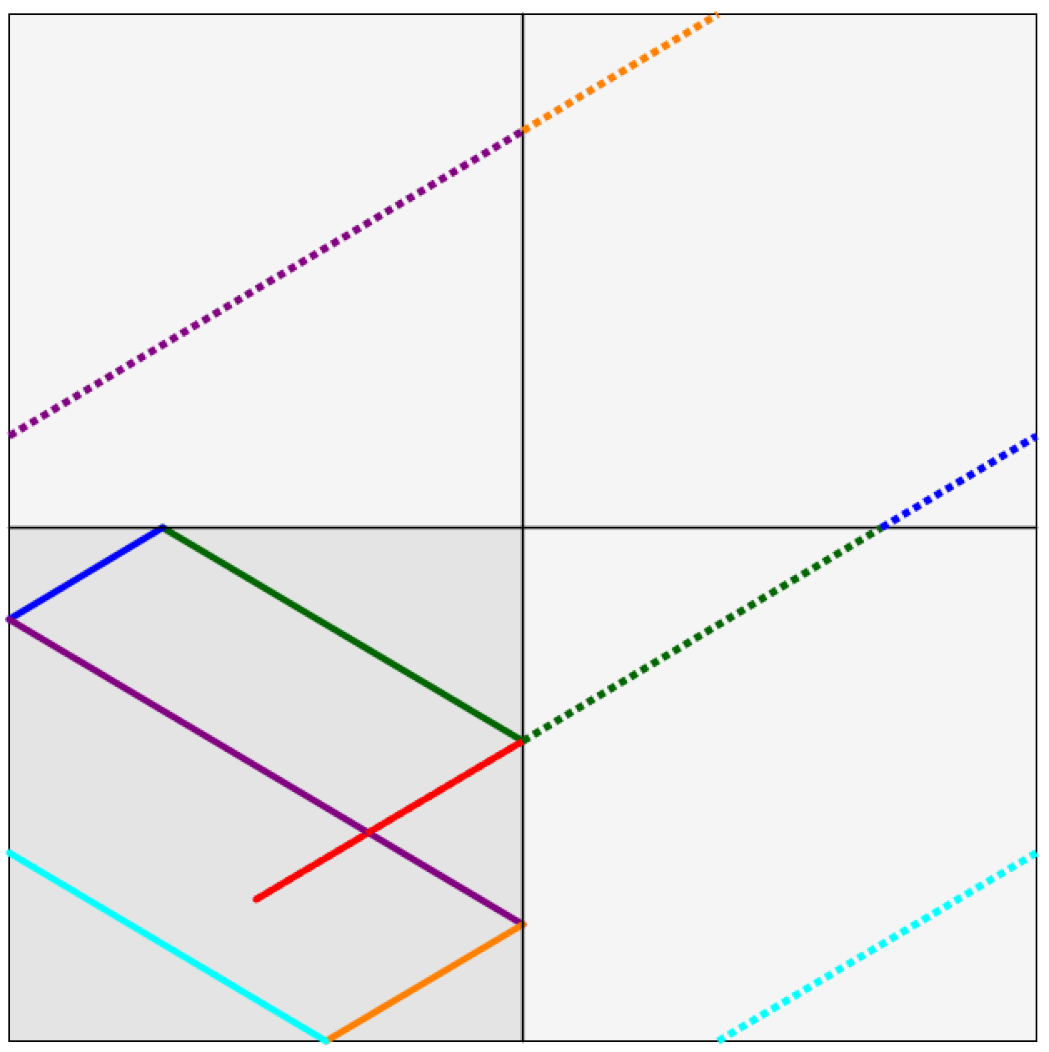
The stabilizer of the standard flat torus (a unit square with opposite sides identified) is . For example, Figure 4 (near the beginning of the previous section) proves that is in the stabilizer. This example illustrates the complexity of the action: applying a large matrix (say of determinant 1) will yield a collection of very long and thin polygons, but it is hard to know when this collection of polygons is equivalent to a more reasonable one.
Translation surfaces have a well defined area, given by the sum of the areas of the polygons. The action of of determinant 1 matrices in preserves the locus of unit area translation surfaces. This locus is not compact, because the polygons can have edges of length going to 0, even while the total area stays constant.
Define
Suppose one wants to know if a translation surface has a vertical line joining singularities (cone points) of length . This is equivalent to the question of whether has a vertical line segment of length 1 joining two singularities.

In fact, for any matrix , the surfaces and are closely related, since one can go back and forth between them using and . Really and are just different perspectives on the same object, in which different features are apparent. To understand from all possible perspectives, we’d like to understand its orbit. However, just from definitions, its not really possible to understand the orbit of a surface. It’s really hard to know, given two surfaces and , if there are large matrices so that the polygons defining can be cut up and reglued to be almost equal to the polygons defining !
4. Renormalization
This section aims to give some of the early motivations and successes of the field. It can be safely skipped and returned to later by anyone eager to get to the modern breakthrough and its applications and connections to other area of mathematics.
Suppose once again that we have a vertical line segment of length on a translation surface . For example, if is the unfolding of a rational polygon, the vertical line might be the unfolding of a billiard trajectory. If one is interested in a line that is not vertical, one can rotate the whole picture (giving a different translation surface) so that it becomes vertical.
Applying results in a translation surface with a vertical segment of length . We are interested in doing this when is very large, and is chosen so the new vertical segment will have length 1. Indeed the point is to do this over and over as gets longer, giving a family of surfaces .
This idea of taking longer and longer trajectories (here vertical lines on the translation surface) and replacing them with bounded length trajectories on new objects is called renormalization, and is a powerful and frequently used tool in the study of dynamical systems. The typical strategy is to transfer some understanding of the sequence of renormalized objects into results on the behavior of the original system. In this case, showing that the geometry of does not degenerate allows good understanding of vertical lines on .
Theorem 4.1 (Masur’s criterion [Mas92]).
Suppose does not diverge to infinity in the stratum. Then every infinite vertical line on is equidistributed on .
“Equidistributed” is a technical term that indicates that the vertical lines becomes dense in without favoring one part of over another. Using this, Kerckhoff-Masur-Smillie [KMS86] were able to show
Theorem 4.2.
In every translation surface, for almost every slope, every infinite line of this slope is equidistributed.
There are some surfaces where much more is true. For example, on the unit square with opposite sides identified, any line of rational slope is periodic, and every line of irrational slope is equidistributed. Genus one translation surfaces are quite special, because acts transitively on the space of genus one translation surfaces. In particular, the orbit of any genus one translation surface is closed, in a trivial way, since the orbit is the entire moduli space.
Theorem 4.3 (Veech Dichotomy).
If is a translation surface with closed orbit, then for all but countably many slopes, every line with that slope is equidistributed. Moreover every line with slope contained in the countable set is periodic.

Veech also showed that the regular -gon with opposite sides identified has closed orbit. However, the property of having a closed orbit is extremely special.
Theorem 4.4 (Masur [Mas82], Veech [Vee82]).
The orbit of almost every translation surface is dense in a connected component of a stratum.
For the experts, we remark that in fact Masur and Veech showed the stronger statement that the action on the loci of unit area surfaces in a connected component of a stratum is ergodic, with respect to a Lebesgue class probability measure called the Masur-Veech measure.
This result of Masur and Veech is not satisfactory from the point of view of billiards in rational polygons, since the set of translation surfaces that are unfoldings of polygons has measure 0.
5. Eskin-Mirzakhani-Mohammadi’s breakthrough
The orbit closure of a translation surface may be a fractal object. While this behavior might at first seem pathological, it is in fact quite typical in dynamical systems. Generally speaking, given a group action it is hugely unrealistic to ask for any understanding of every single orbit, since these may typically be arbitrarily complicated. Thus the following result is quite amazing.
Theorem 5.1 (Eskin-Mirzakhani-Mohammadi [EM, EMM]).
The orbit closure of a translation surface is always a manifold. Moreover, the manifolds that occur are locally defined by linear equations in period coordinates. These linear equations have real coefficients and zero constant term.
Note that although the local period coordinates are not canonical, if a manifold is cut out by linear equations in one choice of period coordinates, it must also be in any other overlapping choice of period coordinates, because the transition map between these two coordinates is a matrix in .
Previously orbit closures had been classified in genus 2 by McMullen. (One open problem remains in genus two, which is the classification of orbits of square-tiled surfaces in .) The techniques of Eskin-Mirzakhani-Mohammadi’s, unlike those of McMullen, are rather abstract, and have surprisingly little to do with translations surfaces. Thus the work of Eskin-Mirzakhani-Mohammadi does not give any information about how many or what sort of submanifolds arise as orbit closures, except for what is given in the theorem statement.
6. Applications of Eskin-Mirzakhani-Mohammadi’s Theorem
There are many applications of Theorem 5.1 to translation surfaces, rational billiards, and other related dynamics systems, for example interval exchange transformations. Here we list just a few of the most easily understood applications.
Generalized diagonals in rational polygons. Let be a rational polygon. A generalized diagonal is a billiard trajectory that begins and ends at a corner of . If is a square, an example is a diagonal of . Let be the number of generalized diagonals in of length at most . It is a folklore conjecture that
exists for every and is non-zero. Previously, Masur had shown that the limsup and liminf are non-zero and finite [Mas90, Mas88]. Eskin-Mirzakhani-Mohammadi give the best result to date: with some additional Cesaro type averaging, the conjecture is true, and furthermore only countably many real numbers may occur as such a limit.
The illumination problem. Given a polygon and two points and , say that is illuminated by if there is a billiard trajectory going from to . This terminology is motivated by thinking of as a polygonal room whose walls are mirrors, and thinking of a candle placed at . The light rays travel along billiard trajectories. We emphasize that the polygon need not be convex.
Lelièvre, Monteil and Weiss have shown that if is a rational polygon, for every there are at most finitely many not illuminated by [LMW].
The Wind Tree Model. This model arose from physics, and is sometimes called the Ehrenfest model. Consider the plane with periodically shaped rectangular barriers (“trees”). Consider a particle (of “wind”) which moves at unit speed and collides elastically with the barriers.
Delecroix-Hubert-Lelièvre have determined the divergence rate of the particle for all choices of size of the rectangular barriers [DHL14]. Without Eskin-Mirzakhani-Mohammadi (and work of Chaika-Eskin [CE]), the best that could proven was the existence of a unspecified full measure set of choices of sizes for which such a result holds.
There are many other examples along these lines, where previously results were known to hold for almost all examples without being known to hold in any particular example, and now with Eskin-Mirzakhani-Mohammadi can be upgraded to hold in all cases.

Applications of Eskin-Mirzakhani’s proof. The ideas that Eskin-Mirzakhani developed have applications beyond moduli spaces of translation surfaces. They are currently being used by Rodriguez-Hertz and Brown to study random diffeomorphisms on surfaces [BRH] and the Zimmer program (lattice actions on manifolds), and are also expected to have applications in ergodic theory on homogeneous spaces.
7. Context from homogeneous spaces
The primary motivation for Theorem 5.1 is the following theorem.
Theorem 7.1 (Ratner’s Theorem).
Let be a Lie group, and let be a lattice. Let be a subgroup generated by unipotent one parameter groups. Then every orbit closure in is a manifold, and moreover is a sub-homogeneous space.
For example, the theorem applies if , , and , where
Ratner’s work confirmed a conjecture of Raghunathan. Special cases of this conjecture had previously been verified by Dani and Margulis, for example for the second choice of above [DM90].
The basic idea behind such proofs is the strategy of additional invariance. Given a closed -invariant set, one starts with two points and very close together, and applies until the points drift apart. The direction of drift is controlled by another one parameter subgroup, and one tries to show that the closed -invariant set is in fact also invariant under the one parameter group that gives the direction of drift. One continues this argument inductively, each time producing another one parameter group the set is invariant under, until one shows that the closed invariant set is in fact invariant under a larger group , and is contained in (and hence equal to) a single orbit. This gives the set in question is homogenous, and in particular a manifold.
Of course, this is in fact very difficult, and complete proofs of Ratner’s Theorem are very long and technical. For one thing, as is the case in the work of Eskin-Mirzakhani, it is in fact too difficult to work directly with closed invariant sets, as we have just suggested. Rather, one first must classify invariant measures. Thus the argument takes place in the realm of ergodic theory, which exactly studies group actions on spaces with invariant measures. See [Mor05, Ein06] for an introduction.
The fundamental requirement of the proof is that orbits of nearby points drift apart slowly and in a controlled way. This is intimately tied to the fact that unipotent one parameter groups are polynomial, as can be seen in the above. Contrast this to the one parameter group
whose orbit closures may be fractal sets.
One might hope to study orbit closures of translation surfaces using the action of
on strata, in analogy to the proof of Ratner’s Theorem. Unfortunately, the dynamics of the action on strata is currently much too poorly understood for this.
8. The structure of the proof
The proof of Theorem 5.1 builds on many ideas in homogeneous space dynamics, including the work of Benoist-Quint [BQ09], and the high and low entropy methods of Einsiedler-Lindenstrauss-Katok [EKL06] (see also the beautiful introduction for a general audience by Venkatesh [Ven08]). Lindenstrauss won the Fields medal in 2010 partially for the development of the low entropy method, and Benoist and Quint won the Clay prize for their work.
Entropy measures the unpredictability of a system that evolves over time.
Define to be the upper triangular subgroup of . The proof of Theorem 5.1 proceeds in two main stages.
In the first, Eskin-Mirzakhani show that any ergodic invariant measure is in fact a Lebesgue class measure on a manifold cut out by linear equations, and must be invariant. (An ergodic measure is an invariant measure which is not the average of two other invariant measures in a nontrivial way. Thus the ergodic measures are the building blocks for all other invariant measures.)
In the second stage, Eskin-Mirzakhani-Mohammadi use this to prove Theorem 5.1, by constructing a -invariant measure on every -orbit closure. By contrast, it is not possible to directly construct an invariant measure on each orbit closure, and this is why the use of is crucial. The algebraic structure of makes it possible to average over larger and larger subsets of and thus produce invariant measures, whereas the more complicated algebraic structure of does not allow this. (The relevant property is that is amenable, while is not.)
In the paper of Eskin-Mirzakhani, which caries out the first stage, the most difficult part is in fact to show -invariant measures are invariant. To do this, extensive entropy arguments are used, partially inspired by the Margulis-Tomanov proof of Ratner’s Theorem [MT94] and to a lesser extent the high and low entropy methods. This part is the technical heart of the argument, and takes almost 100 pages of delicate arguments. One of the morals is that entropy arguments are surprisingly effective in this context, and can be made to work without the use of an ergodic theorem.
Once Eskin-Mirzakhani show that -invariant measures are invariant, they build upon ideas of Benoist-Quint to conclude that every such measure is a Lebesgue class measure on a manifold cut out by linear equations
All together, the proof is remarkably abstract. The only facts used about translation surfaces are formulas for Lyapunov exponents due to Forni [For02]. (The Lyapunov exponents of a smooth dynamical system, in this case the action of on a stratum, measure the rates of expansion and contraction in different directions.) Forni was awarded the Brin prize partially for these formulas, which are of a remarkably analytic nature and arose from an insight of Kontsevich [Kon97]. Eskin-Mirzakhani also make use of a result of Filip [Filb] to handle a volume normalization issue at the end of the proof.
Results which classify invariant measures are rare gems. The arguments are abstract, and their purpose is to rule out nonexistent objects, and thus they cannot be guided by examples. To obtain a truly new measure classification result, one must find truly new ideas from among the sea of ideas which don’t quite work, and the devil is in the details. This is very much the case in the paper of Eskin-Mirzakhani.
9. Relation to Teichmüller theory and algebraic geometry
Every translation surface has, in particular, the structure of a Riemann surface . The extra flat structure is determined by additionally specifying an Abelian differential (a.k.a. holomorphic one form, or global section of the canonical bundle of ). The holomorphic one form is on the polygons, where is the usual coordinate on the plane . It has zeros at the singularities of the flat metric.
Thus every translation surface can be given as a pair . For example, the translation surface given by a square with unit area and opposite edges identified is .
There is a projection map from a stratum of translation surfaces of genus to the moduli space of Riemann surfaces of genus . Under this map, orbits of translation surfaces project to geodesics for the Teichmüller metric. But it is important to note that there is no or action on itself, only on (the strata) of the bundle of Abelian differentials over . This is somewhat analogous to the fact that, given a Riemannian manifold, the geodesic flow is defined on the tangent bundle, and there is no naturally related flow on the manifold itself.
The map has fibers of real dimension two (given by multiplying by any complex number), and thus the projection of a four dimensional orbit to is a two real dimensional object. It turns out that this object is an isometrically immersed copy of the upper half plane in with its hyperbolic metric: such objects are called complex geodesics or Teichmüller disks. Note that Royden showed that the Teichmüller metric is equal to the Kobayashi metric on .
McMullen showed that every orbit closure in genus 2 is either a closed orbit, or an eigenform locus, or a stratum [McM03]. In particular, every orbit closure of genus 2 translation surfaces is a quasi-projective variety. The corresponding statement for is that every complex geodesic is either closed, or dense in a Hilbert modular surface, or dense in .
The appearance of algebraic geometry in the study of orbit closures was unexpected, and arose in very different ways from work of McMullen and Kontsevich. A recent success in this direction is the following, which builds upon Theorem 5.1 and work of Möller [Möl06b, Möl06a].
Theorem 9.1 (Filip [Fila]).
In every genus, every orbit closure is an algebraic variety that parameterizes pairs with special algebro-geometric properties, such as having real multiplication.
Furthermore, Filip’s work gives an algebro-geometric characterization of orbit closures: They are loci of with special algebraic properties, when these loci have maximal possible dimension. (When these loci do not have maximum possible dimension, they do not give orbit closures are not of interest in dynamics.) It is of yet unclear how to make use of this characterization, since calculating the dimension of the relevant sub-varieties of seems to be an incredibly difficult problem, very close to the Schottky problem. Nonetheless Filip’s work means that an equivalent definition of orbit closure can be given to an algebraic geometer, without mentioning flat geometry or even the action!
It is at present a major open problem to classify orbit closures. Progress is ongoing using techniques based on flat geometry and dynamics, see for example [Wri14, NW14, ANW]. One of the key tools is the author’s Cylinder Deformation Theorem, which allows one to produce deformations of a translation surface that remain in the orbit closure, without actually computing any surfaces in the orbit [Wri15a].
10. What to read next
We recommend the two page “What is …measure rigidity” article by Einseidler [Ein09], as well as the eight page note “The mathematical work of Maryam Mirzakhani” by McMullen [McM14] and the 13 page note “The magic wand theorem of A. Eskin and M. Mirzakhani” by Zorich [Zor14, Zor]. There are a large number of surveys on translation surfaces, for example [MT02, Zor06] and the author’s recent introduction aimed at a broad audience [Wri15b]. Alex Eskin has given a mini-course on his paper with Mirzakhani, and notes are available on his website [Esk].
Acknowledgements. I am very grateful to Yiwei She, Max Engelstein, Weston Ungemach, Aaron Pollack, Amir Mohammadi, Barak Weiss, Anton Zorich, and Howard Masur for making helpful comments and suggestions, which lead to significant improvements. This expository article grew out of notes for a talk in the Current Events Bulletin at the Joint Meetings in January 2015. I thank David Eisenbud for organizing the Current Events Bulletin and inviting me to participate, and Susan Friedlander for encouraging me to publish this article.
References
- [ANW] David Aulicino, Duc-Manh Nguyen, and Alex Wright, Classification of higher rank orbit closures in , preprint, arXiv 1308.5879 (2013), to appear in Geom. Top.
- [BQ09] Yves Benoist and Jean-François Quint, Mesures stationnaires et fermés invariants des espaces homogènes, C. R. Math. Acad. Sci. Paris 347 (2009), no. 1-2, 9–13.
- [BRH] Aaron Brown and Federico Rodriguez Hertz, Measure rigidity for random dynamics on surfaces and related skew products, preprint, arXiv 1406.7201 (2014).
- [CE] Jon Chaika and Alex Eskin, Every flat surface is Birkhoff and Oseledets generic in almost every direction, preprint, arXiv 1305.1104 (2014).
- [DHL14] Vincent Delecroix, Pascal Hubert, and Samuel Lelièvre, Diffusion for the periodic wind-tree model, Ann. Sci. Éc. Norm. Supér. (4) 47 (2014), no. 6, 1085–1110.
- [DM90] S. G. Dani and G. A. Margulis, Orbit closures of generic unipotent flows on homogeneous spaces of , Math. Ann. 286 (1990), no. 1-3, 101–128.
- [Ein06] Manfred Einsiedler, Ratner’s theorem on -invariant measures, Jahresber. Deutsch. Math.-Verein. 108 (2006), no. 3, 143–164.
- [Ein09] by same author, What is measure rigidity?, Notices Amer. Math. Soc. 56 (2009), no. 5, 600–601.
- [EKL06] Manfred Einsiedler, Anatole Katok, and Elon Lindenstrauss, Invariant measures and the set of exceptions to Littlewood’s conjecture, Ann. of Math. (2) 164 (2006), no. 2, 513–560.
- [EM] Alex Eskin and Maryam Mirzakhani, Invariant and stationary measures for the action on moduli space, preprint, arXiv 1302.3320 (2013).
- [EMM] Alex Eskin, Maryam Mirzakhani, and Amir Mohammadi, Isolation theorems for -invariant submanifolds in moduli space, preprint, arXiv:1305.3015 (2013).
- [Esk] Alex Eskin, Lectures on the action on moduli space, math.uchicago.edu/~eskin/luminy2012/lectures.pdf.
- [Fila] Simion Filip, Semisimplicity and rigidity of the Kontsevich-Zorich cocycle, preprint, arXiv:1307.7314 (2013).
- [Filb] by same author, Splitting mixed Hodge structures over affine invariant manifolds, preprint, arXiv:1311.2350 (2013).
- [For02] Giovanni Forni, Deviation of ergodic averages for area-preserving flows on surfaces of higher genus, Ann. of Math. (2) 155 (2002), no. 1, 1–103.
- [KMS86] Steven Kerckhoff, Howard Masur, and John Smillie, Ergodicity of billiard flows and quadratic differentials, Ann. of Math. (2) 124 (1986), no. 2, 293–311.
- [Kon97] M. Kontsevich, Lyapunov exponents and Hodge theory, The mathematical beauty of physics (Saclay, 1996), Adv. Ser. Math. Phys., vol. 24, World Sci. Publ., River Edge, NJ, 1997, pp. 318–332.
- [KZ03] Maxim Kontsevich and Anton Zorich, Connected components of the moduli spaces of Abelian differentials with prescribed singularities, Invent. Math. 153 (2003), no. 3, 631–678.
- [LMW] Samuel Lelièver, Thierry Monteil, and Barak Weiss, Everything is illuminated, preprint, arXiv 1407.2975 (2014).
- [Mas82] Howard Masur, Interval exchange transformations and measured foliations, Ann. of Math. (2) 115 (1982), no. 1, 169–200.
- [Mas88] by same author, Lower bounds for the number of saddle connections and closed trajectories of a quadratic differential, Holomorphic functions and moduli, Vol. I (Berkeley, CA, 1986), Math. Sci. Res. Inst. Publ., vol. 10, Springer, New York, 1988, pp. 215–228.
- [Mas90] by same author, The growth rate of trajectories of a quadratic differential, Ergodic Theory Dynam. Systems 10 (1990), no. 1, 151–176.
- [Mas92] by same author, Hausdorff dimension of the set of nonergodic foliations of a quadratic differential, Duke Math. J. 66 (1992), no. 3, 387–442.
- [McM03] Curtis T. McMullen, Billiards and Teichmüller curves on Hilbert modular surfaces, J. Amer. Math. Soc. 16 (2003), no. 4, 857–885 (electronic).
- [McM14] Curtis McMullen, The mathematical work of Maryam Mirzakhani, Proceedings of the International Congress of Mathematicians (Seoul 2014), vol. 1, Kyung Moon SA Co. Ltd., Berlin, 2014, pp. 73–79.
- [Möl06a] Martin Möller, Periodic points on Veech surfaces and the Mordell-Weil group over a Teichmüller curve, Invent. Math. 165 (2006), no. 3, 633–649.
- [Möl06b] by same author, Variations of Hodge structures of a Teichmüller curve, J. Amer. Math. Soc. 19 (2006), no. 2, 327–344 (electronic).
- [Mor05] Dave Witte Morris, Ratner’s theorems on unipotent flows, Chicago Lectures in Mathematics, University of Chicago Press, Chicago, IL, 2005.
- [MT94] G. A. Margulis and G. M. Tomanov, Invariant measures for actions of unipotent groups over local fields on homogeneous spaces, Invent. Math. 116 (1994), no. 1-3, 347–392.
- [MT02] Howard Masur and Serge Tabachnikov, Rational billiards and flat structures, Handbook of dynamical systems, Vol. 1A, North-Holland, Amsterdam, 2002, pp. 1015–1089.
- [NW14] Duc-Manh Nguyen and Alex Wright, Non-Veech surfaces in are generic, Geom. Funct. Anal. 24 (2014), no. 4, 1316–1335.
- [Vee82] William A. Veech, Gauss measures for transformations on the space of interval exchange maps, Ann. of Math. (2) 115 (1982), no. 1, 201–242.
- [Ven08] Akshay Venkatesh, The work of Einsiedler, Katok and Lindenstrauss on the Littlewood conjecture, Bull. Amer. Math. Soc. (N.S.) 45 (2008), no. 1, 117–134.
- [Wri14] Alex Wright, The field of definition of affine invariant submanifolds of the moduli space of abelian differentials, Geom. Topol. 18 (2014), no. 3, 1323–1341.
- [Wri15a] by same author, Cylinder deformations in orbit closures of translation surfaces, Geom. Topol. 19 (2015), no. 1, 413–438.
- [Wri15b] by same author, Translation surfaces and their orbit closures: An introduction for a broad audience, EMS Surv. Math. Sci. 2 (2015), no. 1, 63–108.
- [Zor] Anton Zorich, The magic wand theorem of A. Eskin and M. Mirzakhani, English translation of paper in Gaz. Math., arXiv 1502.05654 (2015).
- [Zor06] by same author, Flat surfaces, Frontiers in number theory, physics, and geometry. I, Springer, Berlin, 2006, pp. 437–583.
- [Zor14] by same author, Le théorème de la baguette magique de A. Eskin et M. Mirzakhani, Gaz. Math. (2014), no. 142, 39–54.