This article is an extended version of a poster article accepted at GECCO 2015, available under DOI: http://dx.doi.org/10.1145/2739482.2764678
Model Selection and Overfitting in Genetic Programming: Empirical Study
Abstract
Genetic Programming has been very successful in solving a large area of problems but its use as a machine learning algorithm has been limited so far. One of the reasons is the problem of overfitting which cannot be solved or suppresed as easily as in more traditional approaches. Another problem, closely related to overfitting, is the selection of the final model from the population.
In this article we present our research that addresses both problems: overfitting and model selection. We compare several ways of dealing with ovefitting, based on Random Sampling Technique (RST) and on using a validation set, all with an emphasis on model selection. We subject each approach to a thorough testing on artificial and real–world datasets and compare them with the standard approach, which uses the full training data, as a baseline.
keywords
machine learning, genetic programming, grammatical evolution, overfitting1 Introduction
In machine learning (ML), the general task is to find a model that is able to predict certain values (unknown in advance) of some objects based on a set of known features of the particular object. There are two kinds of this task: classification and regression. In classification the task is to assign a class (from a finite set of classes) to a given object. In the most general case the class is just a label and there is no other property that the set of classes has (e.g. they need not be orderable). In regression the task is to assign a quantitative value to a given object. In supervised ML, this is achieved using a set of objects with known target class/value to train a particular model.
The need for a correct method to fit the model, tune its metaparameters, select the final model, and estimate its error was recognized a long time ago. In the first attempts, a model was fit to all the available data, and the error of the model on this data was reported. However, as it was soon found out, such a number often underestimated the true error observed on new unseen data, and that such models are not very useful for prediction. This phenomenon – small error reported after training and large error observed on new data – is called overfitting and is caused by the model being fit to the small deviations in the data (e.g. noise) rather then the general trends.
To get an unbiased estimate of the prediction error, the standard practice is to split the available data into two disjoint sets, training and testing, fit the model parameters to the training set, and estimate the prediction error on the testing set. This method is sufficient to get an unbiased estimate of the prediction error for the model, which was constructed by a particular instance of a particular fitting algorithm.
However, there is a need to compare models of various types (results of various fitting algorithms), or models constructed by the same fitting algorithm with different metaparameters. When the testing error estimate is used for model selection, the information about the testing set leaks into the process of model learning, of which the model selection is an unseparable part, and the reported testing error of the final model underestimates the prediction error again. A common basic technique is thus to split the available data into three sets: training, validation, and testing, which serve to fit a particular model, select among available trained models, and estimate the prediction error, respectively.
Genetic Programming (GP) is an evolutionary technique designed to find structured solutions, such as mathematical expressions or computer programs, well fit for a partiuclar task. GP can be applied to ML tasks too, evolving trees wich represent classification or regression models.
1.1 GP as a model fitting algorithm
When GP is used in ML to evolve a model, there are several important differences when compared to ordinary fitting methods:
- •
Ordinary fitting methods often optimize the model parameters only, not its structure, because they rely on the structure of the model. On the one hand, this limits the class of models that can be generated, on the other hand, one can take advantage of this and search classes of different complexities separately. GP, often even with fixed meta-parameters, produces highly free-form models, i.e. models with very different structures with a broad range of complexity.
- •
Ordinary fitting methods are often deterministic, gradient, or best-first search, algorithms, often quickly converging to a local optimum of the objective function. GP is basically a stochastic search, slow, without any guarantee that at least local optimum was found to certain precision.
- •
Ordinary fitting methods usually allow to fit the models with respect to a single training dataset; the error measured on this training data drives the parameter optimization process. Despite theoretically possible, they usually do not allow to store a separate best model so far with respect to a different data set. In GP, on the other hand, it is quite easy to use two or more datasets, one for driving the evolution process, and the other for best model selection.
GP as a ML method can work in two basic modes:
- 1.
GP can be treated as any other ML model fitting algorithm, i.e. we can fix/optimize its meta-parameters, like population size, the set of function symbols to be used, the maximal tree size and depth, etc. The best model in the sense of training error is provided as output. To select the best model, various combinations of meta-parameters can be tried, the resulting models can be evaluated on the validation set, and the best of them is chosen.
Downsides: many algorithm runs, unstable results even for the same data, many meta-parameters value combinations to evaluate.
- 2.
GP can be run in a relatively non-limiting setting allowing it to create models of wide range of complexities, thus searching many model complexity classes at once. The GP algorithm generates many candidate models this way (all population members of all generations); in such a setting, however, the models are likely to overfit the training data and other means are needed to limit the influence of overfitting.
In this article, we would like to concentrate on the second operation mode of GP, comparing several means to limit overfitting, with the goal to asses the influence of individual methods on final model results.
1.2 Related work
Bloat is a phenomenon in GP which can be described as an uncontrolled growth of the program size a very small or no impact on the fitness. Several succesful bloat control techniques were developed (e.g. [9] and [12]). The problem of overfitting was often put into correlation with bloat. This was led by the ideas that bloated models are more likely to be able to fit the noise rather than the short models. However, it was shown [13] that even in a bloat-free envirnoment overfitting can still occur.
2 Overfitting and Model Selection in GP
In GP as a ML algorithm, there are two tasks the evolutionary algorithm must perform:
- 1.
Drive the evolution, i.e. use such fitness that leads to better solutions.
- 2.
Be able to return a single ,,final“ model in any generation.
In the rest of this section we are going to focus on methods of performing these two tasks that are based solely on how the data are handled.
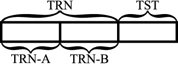
In all approaches we are going to tackle in the rest of the article the data set is initially divided into two parts. The first part we call training data (TRN) and it is the data that are the input to the particular GP algorithm. The second part we call testing data (TST) and it is the data used to evaluate the performance of the final model. The testing data are never available to the algorithm during learning.
For all the methods presented in this article we can further divide the TRN data to two subsets. The first one is used primarily to drive the evolution (i.e. compute fitness) and we call this subset training data A (TRN-A). The other one is used primarily to select the model best so far and we call this subset training data B (TRN-B). These two subsets can either be disjoint or they can overlap or even be identical.
2.1 Standard GP
In the standard approach the whole TRN set is used for both tasks presented in Section 2, i.e. the fitness is the error on the TRN set and the model selection is performed by storing the best model so far with respect to the error TRN set too, i.e. fitness. From the perspective of the data division, all the three sets TRN, TRN-A and TRN-B are identical. The illustration of the data division can bee seen in the Figure 1.

2.2 Validation set based approaches
In the approaches based on validation set the TRN-A and TRN-B sets are disjoint. In these approaches the TRN-B set aids in avoiding overfitting and the model selection at the same time. The illustration of the data division can be seen in the Figure 2.
For the purposes of this article we review two of those approaches: Backwarding [10] and Validation Start [4].
2.2.1 Backwarding
In Backwarding (BW) the evolution is driven only by the TRN-A set, i.e. the fitness is the error over TRN-A. However, the model is selected according to the TRN-B set by storing the best model so far with respect to the error on this set.
This approach has the advantage that the model selection is not based on the data used to learn the model itself and is therefore less likely to produce overfitted models.
2.2.2 Validation Start
In Validation Start (VS) both the evolution and model selection is driven by both sets TRN-A and TRN-B. The fitness is calculated as a weighted sum of two components: error over TRN-A and the absolute difference of the error over TRN-A and the error over TRN-B. The weights and are both random but correlated such that ; they stay fixed for the whole run of the algorithm.
The model selection is done according to the fitness, i.e. the final model is the one with the best fitness.
This approach is motivated by the fact that we want the models to have similar error both on the ,,true“ training data (TRN-A in our terminology) and on the data not used for the actual training.
2.3 Random Sampling based approaches
Random Sampling Technique (RST) [4, 6] is based on the idea of using only a random subset of the training data for fitness evaluation, changing this subset during the evolution.
The model selection is done with respect to the error over the whole TRN set, i.e. TRN-B is identical to TRN.
2.3.1 RST 1/1
In [4] it was shown that the extreme case of using only a single-element subset and changing it every generation, called RST 1/1, produced the best results with respect to the testing error and hence acts as a good technique to control overfitting.
In our terminology of data division, the TRN-A set is composed of a single element chosen randomly from the TRN set and changes every generation. The TRN-B set is identical to the TRN set. The illustration of the data division can be seen in the Figure 3.

2.3.2 Random Interleaved
Random Interleaved (RI) [5] is a technique based on RST 1/1. It is motivated by the fact that in RST only a very small fraction of information is used to learn the model.
In RI, each generation, one of two possibilities of fitness evaluation is randomly chosen. One possibility is identical to RST 1/1, i.e. the fitness is evaluated on a single data point, and the other possibility is identical to standard approach, i.e. the fitness is evaluated on the whole TRN set. The RI method is parametrised by the percentage which indicates the probability of choosing RST 1/1 as the evaluation method in a generation.
In our terminology, in of generations (on average) the TRN-A set is of a single element randomly chosen from TRN and TRN-B is identical to TRN, and in of generations the TRN, TRN-A and TRN-B sets are all identical. The illustration of the data division (for the example of RI 75 %) can be seen in the Figure 4.

2.3.3 RST R
Inspired by the succes of RI 50 % [5] we propose a variant of RST which follows the same motivation as RI but achieves it in a different way. We call our variant RST R (the R stands for ,,random“). It is almost identical to RST but not only the elements of the subset are chosen randomly, the size of this subset is chosen randomly too. The size is drawn from a uniform distribution resulting in using (on average) 50 % of the data points (repetitions counted), almost as in RI 50 %.
2.4 Combining Random Sampling with validation set
All the techniques based on Random Sampling effectively use the whole TRN set both for driving the evolution, which can be seen as the training itself, and for selecting the best model. As we already mentioned in the Section 1, from the point of view of traditional ML methods, this approach is not desirable and can lead to models selected based on underestimated errors.
To improve the algorithms in this area we propose to combine validation set
approach with the Random Sampling approach.
2.4.1 VRST 1/1
VRST 1/1 stands for validation-RST 1/1 and is a variant of RST 1/1 with validation set.
In VRST 1/1, the TRN-A set is a single element changed every generation, like in RST 1/1, but it is drawn from a ,,TRN-A pool“ which is disjoint from the TRN-B set. The best model so far is determined using the TRN-B set. The illustration of data division can be seen in the Figure 5.

2.4.2 VRI
VRI stands for validation-RI and is a variant of RI with validation set.
In VRI, the TRN-A set is either a single element sampled from a ,,TRN-A pool“ or the whole pool (depends on the percentage parameter). The TRN-A pool and TRN-B sets are disjoint. The best model so far is determined using the TRN-B set. The illustration of data division (for the example of VRI 75%) can be seen in the Figure 6.

2.4.3 VRST R
VRST R stands for validation-RST R and is a variant of RST R with validation set.
In VRST R, the TRN-A set is a subset of ,,TRN-A pool“ of random (uniformly distributed) size. The TRN-A pool and TRN-B sets are disjoint. The best model so far is determined using the TRN-B set.
3 Experimental evaluation
In the previous section we reviewed or proposed various approaches to prevent overfitting. In order to find out how each approach works, we conducted a series of experiments on various datasets. The rest of this section describes the used datasets and the setup of the algorithms and experiments.
3.1 Data sets
For the testing of all the algorithms we used a set of six datasets.
Two Spirals (TS), Cluster in Cluster (CIC) and Halfkernel (HK) are binary classification datasets generated by MATLAB scripts from [7].
Sphere (SPH) is a regression dataset defined as
where each is independently randomly sampled from interval and is a random value drawn uniformly from interval .
Forest Fires (FF) [2] retrieved from the UCI repository [1] is a real-world regression dataset where the task is to predict the burned area of the forest. All features are numeric except the 3rd and 4th features which are month (,,jan“ to ,,dec“) and day (,,mon“ to ,,sun“) respectively. These were transformed to numbers by mapping the month to the numbers 1 to 12 (,,jan“ being mapped to 1, ,,dec“ being mapped to 12) and day to the numbers 1 to 7 (,,mon“ being mapped to 1, ,,sun“ being mapped to 7).
Wisconsin Diagnostic Breast Cancer (WDBC) retrieved from the UCI repository [1] is a real-world binary classification dataset where the task is to state a diagnosis (malignant/benign) based on numeric features computed from digitized image of a breast mass.
A summary description of the datasets is in Table 1.
| dataset | artificial | task | # instances | # features |
|---|---|---|---|---|
| TS | yes | clas. | 3000 | 2 |
| CIC | yes | clas. | 1240 | 2 |
| HK | yes | clas. | 1200 | 2 |
| SPH | yes | regr. | 1500 | 30 |
| FF | no | regr. | 517 | 12 |
| WDBC | no | clas. | 569 | 30 |
All classification tasks are binary ones (i.e. there are two classes to classify).
3.2 GP algorithm and setup
For the GP algorihm we used Grammatical Evolution [11]. The setup of the algorithm was identical in all the used methods and datasets and can be seen in the Table 2.
| initial maximum genotype length | 100 codons |
|---|---|
| codon value range | 0 to 255 |
| pop. size | 500 |
| generations | 200 |
| selection | tournament of 4 |
| crossover prob. | 0.5 |
| crossover type | single-point (ripple) |
| mutation prob. (per codon) | 0.1 |
| mutation type | change codon to random number from range |
| pruning prob. | 0.2 |
| duplication prob. | 0.2 |
| maximum wraps | 0 (wrapping disabled) |
For all the experiments we used the same grammar which is described in the Appendix A.
For regression tasks, the output of the evolved expression was directly used as the estimated value. For classification tasks (only binary classification, see Section 3.1), if the output of the evolved expression was less than 0 then the first class was assigned, else was the second class.
The (V)RI methods’ percentage paremeter was set to 60% as it is a middle ground between 50% and 75% that were among the most successful ones in [5].
If any solution produced a mathematical error (e.g. division by zero or a logarithm
of negative number) it received infinite fitness (which is always the worst).
3.3 Setup of the experiments
For each dataset every algorithm was run 96 times. The TRN/TST division ratio was fixed to 70%/30% for all runs of all algorithms on all datasets. The division was different for each run of an algorithm but runs with equal number had the same division (e.g. the first runs of RST 1/1 and VRST R on TS dataset had the same TRN and TST subsets).
Algorithms BW, VS, VRI, VRST R and VRST 1/1 had the TRN-A/TRN-B division ratio fixed to 50%/50%, again different in every run but equal in corresponding runs of all the algorithms.
4 Results


The overall results can be seen in the Table 3. The ,,rank“ column in this table is the rank of the method on the particular dataset. The rank was determined using the one-sided Mann-Whitney U test on the final TST errors, pairwise among all methods on the particular dataset, with the level of significance : methods with equal ranks are not statistically significantly different; if two methods, A and B, have ranks and such that then method A is statistically significantly better than method B.
| TST error | TRN error | tree size | |||||||||
|---|---|---|---|---|---|---|---|---|---|---|---|
| dataset | rank | method | median | mean | stddev | median | mean | stddev | median | mean | stddev |
| TS | 1 | STD | 0.326 | 0.326 | 0.014 | 0.321 | 0.321 | 0.006 | 5 | 6.844 | 4.913 |
| BW | 0.327 | 0.328 | 0.014 | 0.325 | 0.324 | 0.006 | 6 | 6.677 | 3.862 | ||
| RST 1/1 | 0.325 | 0.325 | 0.013 | 0.324 | 0.324 | 0.006 | 3 | 3.604 | 2.255 | ||
| VRST 1/1 | 0.326 | 0.326 | 0.014 | 0.325 | 0.325 | 0.005 | 3 | 3.365 | 2.304 | ||
| RST R | 0.324 | 0.325 | 0.013 | 0.324 | 0.323 | 0.006 | 3 | 4.229 | 3.197 | ||
| VRST R | 0.324 | 0.324 | 0.013 | 0.325 | 0.324 | 0.006 | 3 | 4.458 | 5.013 | ||
| RI 60% | 0.326 | 0.325 | 0.013 | 0.324 | 0.324 | 0.006 | 3 | 3.740 | 3.079 | ||
| VRI 60% | 0.327 | 0.326 | 0.013 | 0.325 | 0.325 | 0.005 | 3 | 3.396 | 2.693 | ||
| 2 | VS | 0.331 | 0.333 | 0.018 | 0.326 | 0.330 | 0.018 | 8 | 8.135 | 5.364 | |
| CIC | 1 | STD | 0.055 | 0.054 | 0.044 | 0.054 | 0.051 | 0.042 | 11 | 11.500 | 3.393 |
| 2 | BW | 0.094 | 0.093 | 0.038 | 0.095 | 0.089 | 0.032 | 10 | 10.427 | 2.944 | |
| VS | 0.099 | 0.107 | 0.069 | 0.094 | 0.104 | 0.069 | 10 | 10.542 | 3.346 | ||
| RST R | 0.099 | 0.121 | 0.074 | 0.099 | 0.117 | 0.069 | 9 | 9.271 | 3.144 | ||
| VRST R | 0.106 | 0.132 | 0.071 | 0.107 | 0.134 | 0.068 | 8 | 8.823 | 3.369 | ||
| 3 | RI 60% | 0.286 | 0.292 | 0.068 | 0.291 | 0.292 | 0.059 | 6 | 6.854 | 4.282 | |
| 4 | RST 1/1 | 0.319 | 0.329 | 0.060 | 0.308 | 0.324 | 0.050 | 4 | 5.552 | 3.825 | |
| VRST 1/1 | 0.306 | 0.326 | 0.065 | 0.301 | 0.321 | 0.055 | 4 | 5.396 | 2.871 | ||
| VRI 60% | 0.294 | 0.308 | 0.070 | 0.291 | 0.304 | 0.060 | 4 | 5.292 | 2.768 | ||
| HK | 1 | STD | 0.188 | 0.178 | 0.066 | 0.175 | 0.174 | 0.059 | 12 | 12.417 | 4.106 |
| 2 | BW | 0.246 | 0.235 | 0.050 | 0.244 | 0.231 | 0.042 | 9 | 10.281 | 4.436 | |
| VS | 0.254 | 0.244 | 0.054 | 0.248 | 0.241 | 0.050 | 9 | 9.812 | 4.409 | ||
| 3 | RST 1/1 | 0.267 | 0.266 | 0.021 | 0.267 | 0.267 | 0.009 | 3 | 3.833 | 2.638 | |
| VRST 1/1 | 0.265 | 0.267 | 0.021 | 0.268 | 0.269 | 0.011 | 3 | 4.240 | 4.301 | ||
| RST R | 0.267 | 0.263 | 0.028 | 0.262 | 0.258 | 0.022 | 6 | 6.792 | 4.410 | ||
| VRST R | 0.261 | 0.263 | 0.021 | 0.265 | 0.265 | 0.011 | 4 | 5.385 | 3.310 | ||
| RI 60% | 0.265 | 0.266 | 0.021 | 0.267 | 0.267 | 0.011 | 3 | 3.969 | 2.412 | ||
| VRI 60% | 0.267 | 0.266 | 0.020 | 0.268 | 0.268 | 0.011 | 3 | 4.010 | 2.606 | ||
| SPH | 1 | STD | 5.141 | 5.821 | 6.144 | 5.127 | 5.069 | 0.529 | 8 | 9.646 | 3.995 |
| BW | 5.125 | 5.122 | 0.399 | 5.128 | 5.113 | 0.279 | 8 | 9.354 | 3.305 | ||
| VS | 5.163 | 5.667 | 2.202 | 5.152 | 5.601 | 2.130 | 9 | 9.854 | 3.043 | ||
| RST R | 5.132 | 5.150 | 0.137 | 5.126 | 5.122 | 0.169 | 8 | 9.000 | 2.220 | ||
| VRST R | 5.125 | 5.330 | 1.841 | 5.129 | 5.213 | 0.829 | 8 | 8.833 | 2.260 | ||
| RI 60% | 5.222 | 5.434 | 0.517 | 5.168 | 5.400 | 0.496 | 8 | 8.167 | 2.360 | ||
| VRI 60% | 5.172 | 5.321 | 0.388 | 5.185 | 5.321 | 0.387 | 8 | 8.062 | 2.112 | ||
| 2 | RST 1/1 | 5.253 | 5.450 | 0.507 | 5.191 | 5.444 | 0.509 | 8 | 8.167 | 2.482 | |
| VRST 1/1 | 5.229 | 5.462 | 0.582 | 5.180 | 5.462 | 0.574 | 8 | 8.302 | 1.985 | ||
| FF | 1 | STD | 2.134 | 13.529 | 47.349 | 0.000 | 0.103 | 0.274 | 7 | 8.135 | 3.732 |
| BW | 2.720 | 18.004 | 78.684 | 0.000 | 4.599 | 31.233 | 7 | 9.010 | 6.141 | ||
| VS | 3.058 | 27.150 | 24.220 | 0.000 | 0.541 | 1.463 | 7 | 8.417 | 3.749 | ||
| VRST R | 4.813 | 15.634 | 48.126 | 4.859 | 73.167 | 540.151 | 7 | 8.354 | 6.614 | ||
| 2 | RST 1/1 | 6.980 | 545.889 | 35.743 | 5.082 | 12.235 | 16.959 | 5 | 7.375 | 6.460 | |
| VRST 1/1 | 7.777 | 27.982 | 59.345 | 9.201 | 13.691 | 22.369 | 5 | 7.104 | 5.717 | ||
| RST R | 6.376 | 22.297 | 45.114 | 1.000 | 8.708 | 14.632 | 7 | 7.562 | 4.091 | ||
| RI 60% | 6.986 | 17.076 | 31.035 | 5.936 | 11.064 | 13.201 | 3 | 6.344 | 4.847 | ||
| VRI 60% | 6.967 | 20.687 | 41.611 | 6.086 | 11.521 | 20.178 | 5 | 7.250 | 6.259 | ||
| WDBC | 1 | STD | 0.076 | 0.078 | 0.020 | 0.065 | 0.066 | 0.012 | 8 | 8.083 | 3.201 |
| BW | 0.082 | 0.082 | 0.021 | 0.075 | 0.075 | 0.013 | 6 | 6.958 | 3.054 | ||
| 2 | VS | 0.096 | 0.109 | 0.058 | 0.080 | 0.100 | 0.059 | 6 | 7.167 | 4.410 | |
| 3 | RST R | 0.193 | 0.215 | 0.111 | 0.187 | 0.209 | 0.106 | 6 | 6.729 | 4.826 | |
| VRST R | 0.234 | 0.230 | 0.110 | 0.230 | 0.235 | 0.105 | 5 | 5.656 | 4.154 | ||
| 4 | RST 1/1 | 0.310 | 0.279 | 0.086 | 0.318 | 0.279 | 0.079 | 3 | 4.792 | 5.651 | |
| VRST 1/1 | 0.310 | 0.288 | 0.078 | 0.327 | 0.290 | 0.074 | 3 | 4.260 | 4.223 | ||
| RI 60% | 0.295 | 0.273 | 0.086 | 0.313 | 0.269 | 0.086 | 3 | 5.490 | 5.018 | ||
| VRI 60% | 0.307 | 0.270 | 0.090 | 0.304 | 0.265 | 0.085 | 3 | 5.156 | 5.135 | ||
4.1 Performance of standard approach
Surprisingly, on all the datasets, the standard approach was either the best or in the group of the best approaches. This result is contradictory to [4, 6] and [5]. However, in [4] the approaches were tested only on a single one-dimensional artificial dataset, and in [6, 5] the approaches were tested on three real-world high-dimensional datasets. In our experiments both artificial and real-world datasets of 2 to 30 dimensions were used.
This result suggests that the benefit of RST-based approaches is data-dependent and general conclusion cannot be made based on the experiments carried out so far.
4.2 Benefit of using a validation set
The only case where validation set variant of a method was statistically significantly better than its non-validation set variant was the VRST R on FF dataset. In all other cases the validation and non-validation variants of the algorithms were not statistically significantly different.
This result suggests that using a validation set does not bring much benefit, at least on the datasets and with setup used in these experiments. One of the reasons might be the tradeoff between overfitting prevention and giving the algorithm enough information to be able to learn.
4.3 Random-sized subsets
In all the experiments there was no case of the (V)RST R being statistically significantly worse than (V)RST 1/1 or (V)RI 60%. On the other hand, on CIC and WDBC datasets the (V)RST R was statistically significantly better than both (V)RI 60% and (V)RST 1/1 and on FF dataset VRST R was statistically significantly better than all other RST-based approaches.
This result suggests that using random-sized subsets might be more beneficial than using either only a single-element subsets or switching between the full set and single-element subset. The reason for this might be that when using a single-element subset the number of fitness cases (meaning the part of the data the solutions are to classify/model) the algorithm can encounter is much smaller than in the case of random-sized subsets, causing lower variability of the actual training data.
5 Conclusions
In this article we further explored the issue of overfitting in Genetic Programming. In detail we discussed the ways the data are handled and based on two patterns - validation set and random sampling - we proposed two new approaches: RST with random-sized subsets and using a validation set in RST-based techniques, including the combination of both.
The RST random was based on the idea that using only single element or only the full training set makes the number of fitness cases small. RST R uses not only randomly chosen elements of the subsets but the size of the subsets is random too.
Bringing validation set to RST-based techniques was based on the idea that selecting the model with respect to the actual training set could bring unwanted bias towards the training data. In the variants with validation set the model selection and the actual learning are isolated, preventing such bias.
We have carried out a series of experiments with all the presented approaches on six datasets, both artificial and real-world, both for classification and regression.
The most important result is that the standard approach, i.e. learn and select model on the whole training set all the time, came out as either the best or among the best approaches on all the datasets. This result is contradictory to the previous articles [4, 6, 5] where this approach performed poorly. This indicates that the technique performance could be highly data dependent and therefore we think no general conclusion about the benefit of random sampling can be made. This result asks for further investigation to find out which aspects of the data cause various approaches to perform well or poorly.
The second result is that our idea of using a validation set did not prove to be significantly beneficial. There was only a single case where the validation set variant significantly outperformed the non-validation variant. However, this approach also requires further investigation because it could also be data dependent and also because we tested only one division ratio. Different setup could have (or not) a significant impact on the performance of such methods.
The third result is the good performance of random-sized subsets with respect to the other two RST-based methods. There was no case the random-sized subsets caused worse performance than the other two methods and in some cases there was a significant difference to the favor of the random-sized subsets. However, this could be data dependent too, and further investigation is also needed. Another aspect of this method is the distribution of the subset size. We used uniform distribution but other distributions, e.g. favoring smaller subsets, could prove even more beneficial.
6 Acknowledgments
This work was supported by the Grant Agency of the Czech Technical University
in Prague, grant No.
SGS14/194/OHK3/3T/13.
Access to computing and storage facilities owned by parties and projects
contributing to the National Grid Infrastructure MetaCentrum, provided under
the programme
"Projects of Large Infrastructure for Research, Development, and
Innovations" (LM2010005), is greatly appreciated.
References
- [1] K. Bache and M. Lichman. UCI machine learning repository, 2013. http://archive.ics.uci.edu/ml.
- [2] P. Cortez and A. d. J. R. Morais. A data mining approach to predict forest fires using meteorological data. 2007.
- [3] C. Gathercole and P. Ross. Dynamic training subset selection for supervised learning in genetic programming. In Parallel Problem Solving from Nature — PPSN III, volume 866 of Lecture Notes in Computer Science, pages 312–321. Springer Berlin Heidelberg, 1994.
- [4] I. Gonçalves and S. Silva. Experiments on controlling overfitting in genetic programming. In 15th Portuguese Conference on Artificial Intelligence, October 2011.
- [5] I. Gonçalves and S. Silva. Balancing learning and overfitting in genetic programming with interleaved sampling of training data. In Genetic Programming, volume 7831 of Lecture Notes in Computer Science, pages 73–84. Springer Berlin Heidelberg, 2013.
- [6] I. Gonçalves, S. Silva, J. Melo, and J. Carreiras. Random sampling technique for overfitting control in genetic programming. In Genetic Programming, volume 7244 of Lecture Notes in Computer Science, pages 218–229. Springer Berlin Heidelberg, 2012.
- [7]
J. Kools.
6 functions for generating artificial
datasets
(mathworks.com/matlabcentral/fileexchange/41459). MATLAB Central File Exchange, Retrieved December 17, 2014. http://www.mathworks.com/matlabcentral/ fileexchange/41459. - [8] Y. Liu and T. Khoshgoftaar. Reducing overfitting in genetic programming models for software quality classification. In High Assurance Systems Engineering, 2004. Proceedings. Eighth IEEE International Symposium on, pages 56–65, March 2004.
- [9] R. Poli and N. McPhee. Parsimony pressure made easy: Solving the problem of bloat in gp. In Theory and Principled Methods for the Design of Metaheuristics, Natural Computing Series, pages 181–204. Springer Berlin Heidelberg, 2014.
- [10] D. Robilliard and C. Fonlupt. Backwarding: An overfitting control for genetic programming in a remote sensing application. In Artificial Evolution, volume 2310 of Lecture Notes in Computer Science, pages 245–254. Springer Berlin Heidelberg, 2002.
- [11] C. Ryan, J. Collins, and M. Neill. Grammatical evolution: Evolving programs for an arbitrary language. In Genetic Programming, volume 1391 of Lecture Notes in Computer Science, pages 83–96. Springer Berlin Heidelberg, 1998.
- [12] S. Silva and E. Costa. Dynamic limits for bloat control in genetic programming and a review of past and current bloat theories. Genetic Programming and Evolvable Machines, 10(2):141–179, 2009.
- [13] L. Vanneschi and S. Silva. Using operator equalisation for prediction of drug toxicity with genetic programming. In Progress in Artificial Intelligence, volume 5816 of Lecture Notes in Computer Science, pages 65–76. Springer Berlin Heidelberg, 2009.
Appendix A Grammar
The grammar used for all experiments was of the following form (the italic texts are comments, not part of the grammar):
| <expr> | ::= | (<expr> <biop> <expr>) | |
|---|---|---|---|
| | | (<unop> <expr>) | ||
| | | <var> | ||
| | | <const> | ||
| <biop> | ::= | + | |
| | | - | ||
| | | * | ||
| | | / | ||
| | | ^ |
exponentiation | |
| <unop> | ::= | ln | natural logarithm |
| | | exp | natural exponential () | |
| | | - | unary minus | |
| | | abs | absolute value | |
| <var> | ::= | x1 | x2 | ... | |
| <const> | ::= | -1 | 1 | |
where x1, x2, etc. are the feature variables of the particular dataset. \balancecolumns