ESO Valuation with Job Termination Risk and Jumps in Stock Price
Abstract
Employee stock options (ESOs) are American-style call options that can be terminated early due to employment shock. This paper studies an ESO valuation framework that accounts for job termination risk and jumps in the company stock price. Under general Lévy stock price dynamics, we show that a higher job termination risk induces the ESO holder to voluntarily accelerate exercise, which in turn reduces the cost to the company. The holder’s optimal exercise boundary and ESO cost are determined by solving an inhomogeneous partial integro-differential variational inequality (PIDVI). We apply Fourier transform to simplify the variational inequality and develop accurate numerical methods. Furthermore, when the stock price follows a geometric Brownian motion, we provide closed-form formulas for both the vested and unvested perpetual ESOs. Our model is also applied to evaluate the probabilities of understating ESO expenses and contract termination.
Keywords: employee stock option, job termination, Lévy processes, Fourier transform
JEL Classification: C41, G13, J33
Mathematics Subject Classification (2010): 60G40, 62L15, 91G20, 91G80
1 Introduction
Employee stock options (ESOs) are an integral part of executive compensation in the United States. The primary objective is to align the interests between the executives and the firm. According to Frydman and Jenter (2010), stock options account for 25% of the total compensation package of CEOs in 2008. In Table 1, we see that the percentage of S&P 500 companies granting ESOs remains above 73% in 2011, despite a decline from 93% in 2000. The cost of these options can potentially be very burdensome to the shareholders. In view of this, the Financial Accounting Standards Board (FASB) has passed regulations to require firms to estimate and report the granting cost of ESOs.
Typically, ESOs are early-exercisable long-dated call options written on the company stock. To maintain the incentive effect, the firm usually imposes a vesting period that prohibits the employee from exercising the option. During the vesting period, the employee’s departure from the firm will result in forfeiture of the option (i.e. it becomes worthless). After the vesting period, when the employee leaves the firm, the ESO will expire though the employee can choose to exercise if the option is in the money11 1 See, for example, “A Detailed Overview of Employee Ownership Plan Alternatives” by The National Center for Employee Ownership (http://www.nceo.org). . Table 1 summarizes the average vesting period and average maturity of ESOs granted by S&P 500 companies over 2000-2011. As we can see, the vesting period has been consistently close to 2 years, while the average maturity has decreased from 9-10 years to 8 years over a decade.
The key to ESO valuation involves modeling the employee’s voluntary exercise strategy as well as job termination time, especially since the option is typically terminated prior to the contractual expiration date. Moreover, the possibility of future employment shock can influence the employee’s decision to exercise now or later. In fact, the FASB guideline22 2 See Sect. A.16, FASB Statement 123R (revised 2004), available on http://www.fasb.org/summary/stsum123r.shtml. also recommends that any reasonable ESO valuation model incorporate “the effects of employees’ expected exercise and post-vesting employment termination behavior.”
In this paper, we study a valuation framework that incorporates the common ESO features of vesting period, early exercise and job termination risk, while allowing for different price dynamics with jumps. Specifically, we model the arrival of the employment shock by an exogenous jump process, and formulate the American-style ESO as an optimal stopping problem with possible forced exercise prior to expiration date. Our valuation problem is studied under a class of exponential Lévy price processes, rather than limiting to the GBM framework commonly found in the literature (see e.g. Hull and White (2004); Cvitanić et al. (2008); Carpenter et al. (2010)). Under different job termination intensity assumptions (constant or stochastic), we analyze the corresponding free boundary problems in terms of an inhomogeneous partial integro-differential variational inequality (PIDVI), and discuss the computational methods to solve for the option value as well as the optimal exercise strategy. Analytically and numerically, we find that with higher job termination risk it is optimal for the holder to voluntarily accelerate ESO exercise. For risk analysis, we also apply our numerical schemes to calculate the probability of cost exceedance and the probability of contract termination under various scenarios.
In existing literature, there are several major approaches to model the exercise timing of ESOs. The first approach assigns an ad hoc exercise boundary for the ESO holder. In other words, the ESO exercise is characterized by the first passage time of underlying stock price to a pre-specified level, which is independent of the employee’s job termination rate or other model parameters. The main advantage of this approach is the availability of closed-form formulas for the ESO value. Additionally, one can also incorporate a random job termination time, as in Hull and White (2004); Cvitanić et al. (2008), but it would not directly affect the voluntary exercise boundary.
To incorporate the employee’s risk attitude, the utility maximization approach derives the employee’s exercise strategy from a portfolio optimization problem that accounts for the employee’s risk aversion and hedging restrictions (Huddart, 1994; Chance and Yang, 2005; Grasselli and Henderson, 2009; Leung and Sircar, 2009; Carpenter et al., 2010). The utility-maximizing exercise boundary represents the optimal voluntary exercise timing for the risk-averse employee. From the firm’s perspective, the ESO cost is computed by risk-neutral expectation assuming the option will be exercised at the utility-maximizing boundary or job termination time, whichever is earlier.
On the other hand, the intensity-based approach does not distinguish voluntary and involuntary exercise, and model the contract termination by a single random time, characterized by the first arrival time of an exogenous jump process. In the literature, Jennergren and Naslund (1993) model the exercise time using an exogenous Poisson process, and Carr and Linetsky (2000) propose an intensity-based model for ESO valuation where both job termination and voluntary exercise intensities are functions of the company stock price. In the theoretical study by Szimayer (2004), the employee is allowed to optimally select a voluntary exercise time, while the sudden departure is represented by an exogenous Cox process. In practice, the job termination intensity specification depends on the firm’s history and estimation methodology. For empirical studies on the early exercise patterns of ESOs, we refer to Huddart and Lang (1996); Marquardt (2002); Bettis et al. (2005).
| Year | % of S&P500 companies | Avg. vesting period | Avg. Maturity |
| granting ESOs | (years) | (years) | |
| 2000 | 92.98% | 2.00 | 9.24 |
| 2001 | 94.35% | 2.22 | 9.28 |
| 2002 | 93.56% | 2.18 | 9.53 |
| 2003 | 89.59% | 2.18 | 10.17 |
| 2004 | 88.09% | 2.03 | 8.66 |
| 2005 | 75.34% | 2.16 | 8.61 |
| 2006 | 81.30% | 2.12 | 7.86 |
| 2007 | 77.33% | 2.18 | 8.14 |
| 2008 | 76.31% | 2.38 | 7.35 |
| 2009 | 75.30% | 2.16 | 8.41 |
| 2010 | 72.69% | 2.32 | 8.71 |
| 2011 | 73.39% | 2.16 | 8.07 |
We consider the ESO as an American call option with a possible sudden forfeiture or forced exercise due to job termination. In contrast to many existing ESO models, we study a versatile valuation framework that is compatible for a wide class of Lévy price processes, including Merton (1976) and Kou (2002) jump diffusions, as well as Variance Gamma (VG) (Madan et al. (1998)) and CGMY (Carr et al. (2002)) models, in addition to GBM that is commonly found in the literature including those cited above. This allows us to study the combined effect of jumps in stock price and job termination intensity on the ESO value and optimal exercise boundary. Moreover, our model provides the end-user, i.e. the firm, the flexibility in choosing the appropriate price model (within a general Lévy class) for the underlying stock. Currently, the FASB permits the use of the Black-Scholes formula with the ESO’s contractual term replaced by its average life, as well as a number of variations33 3 See Sect. A.25, FASB Statement 123R (revised 2004).. In this regard, our paper offers an alternative valuation approach that accounts for both voluntary exercise and job termination risk along with various choices of models for the company stock price.
The ESO valuation problem can be considered as an extension to the pricing of American options under Lévy processes; see Pham (1997), Hirsa and Madan (2004), Bayraktar and Xing (2009), Lord et al. (2008), and Lamberton and Mikou (2008), among others. For vested ESOs, the job termination arrival forces the employee to exercise immediately. This leads to an optimal stopping problem with forced exit. In terms of the variational inequality for the option value, this restriction gives rise to an inhomogeneous term that depends on both the option payoff and job termination intensity. When the stock price follows a geometric Brownian motion, we provide the closed-form formulas for both the vested and unvested perpetual ESO costs. The optimal exercise threshold can be determined uniquely from a polynomial equation, and it admits an explicit expression in the case without job termination risk.
In order to compute the ESO value and exercise boundary, we apply the Fourier Stepping Timing (FST) approach, whereby the associated inhomogeneous PIDVI is simplified by Fourier transform and the optimal exercise price is determined in each time step. Jackson et al. (2008) apply this approach to price European, American, and barrier options under a number of Lévy models. For our ESO valuation problem, the structure of the inhomogeneous PIDVI varies under different job termination intensity specifications. In particular, if the intensity is affine in the (log) stock price, then the inhomogeneous PIDE for the ESO in the continuation region can be simplified to an inhomogeneous PDE. In the constant intensity case, we further reduce the associated PIDE into an ODE. These observations lead to several efficient numerical algorithms for valuation. In all these cases, we compare with the numerical results from an implicit-explicit finite difference method for valuing the ESO. To this end, we refer to the finite difference methods for pricing American options under Lévy or jump diffusion models, including Cont and Voltchkova (2003); d’Halluin et al. (2003); Hirsa and Madan (2004), and Forsyth et al. (2007).
Firms typically expense the granted ESOs according to a fixed schedule, such as quarterly or annually, but the cost of an ESO changes over time depending on the stock price movement. From the firm’s perspective, a rise in the ESO value implies a higher expected cost of compensation as compared to the initially reported value. On the other hand, existing ESOs can be either exercised voluntarily by the employee, or terminated due to employment termination. This motivates us to study (i) the probability that the ESO cost will exceed a given level in the future, and (ii) the contract termination probability. The ESO cost exceedance probability bears similarity to the loss probability used in classical value-at-risk calculation. The contract termination probability sheds light on the likelihood that the firm will have to pay the employee over a future horizon, from a week to a few years. We apply Fourier transform based methods to compute these probabilities under constant job termination intensity, and we show the connection between our approach and that developed by Carr and Madan (1999) in the computation of these probabilities.
The rest of the paper is structured as follows. In Section 2, we formulate the ESO valuation framework under Lévy price dynamics. In Section 3, we discuss the Fourier transform based numerical methods for ESO valuation. In Section 4, we discuss the valuation problem under stochastic job termination intensity. In Section 5, we analyze and evaluate the probability of ESO cost exceedance and the probability of contract termination. In Section 6, we provide closed-form formulas for the vested and unvested perpetual ESO costs under the lognormal stock price model. Section 7 concludes the paper.
2 Model Formulation
In the background, we fix a probability space satisfying the usual conditions of right continuity and completeness, where is the historical probability measure. Let be a Lévy process, which admits the well-known Lévy-Itô decomposition (Sato, 1999, p.119):
| (2.1) |
where is a standard Brownian motion under , and the jump terms are given by
| (2.2) | ||||
| (2.3) |
The characteristic triplet () of consists of the constant drift and volatility , along with the Lévy measure . In (2.2) and (2.3), the Poisson random measure counts the number of jumps of size occurring at time , and is the associated compensator.
The characteristic exponent of is given by the Lévy-Khintchine formula (Sato, 1999, p.119):
| (2.4) |
With this, the characteristic function of is . We denote as the filtration generated by .
In Table 2, we summarize the Lévy densities and characteristic exponents for several well-known Lévy models that will be used in this paper. In the GBM model (Black and Scholes, 1973), the Lévy density is absent as the stock price has no jumps. The Merton (1976) jump diffusion model features normally distributed jump sizes, while the Kou (2002) model assumes a double exponential distribution for the jump sizes. In contrast, under the Variance Gamma (VG) model (Madan et al. (1998)) and CGMY model (Carr et al. (2002)), the stock price follows a pure jump process with infinite activity.
| Model | Lévy Density | Characteristic Exponent |
| GBM | N/A | |
| Merton | ||
| Kou | ||
| VG | ||
| CGMY |
The company stock price is modeled by an exponential Lévy process
with constant initial stock price . In addition, we assume positive constant interest rate and non-negative dividend rate . For ESO valuation, we work with a risk-neutral pricing measure such that
| (2.5) |
where is given in (2.4) with replaced by
| (2.6) |
and is the Lévy measure under .
2.1 Payoff Structure
Figure 1 illustrates the payoff structure of an ESO with strike , vesting period of years, and expiration date . During the vesting period, the ESO is not exercisable and is forfeited if the employee leaves the firm. As soon as the option is vested (at or after time ), the employee can exercise the option at any time prior to the expiration date , but will also be forced to exercise immediately upon job termination. We model the employee’s job termination time by an exponential random variable with rate parameter , and assume that and are independent. The case of stochastic job termination will be discussed in Section 4.

2.2 ESO Cost
The value of a vested ESO at time is given by
| (2.7) | ||||
| (2.8) |
where is the set of stopping times taking values in , and denotes the conditional expectation with . In other words, after the vesting period, the employee faces an optimal stopping problem similar to that for an American call option, but is subject to forced early exercise due to sudden job termination. From (2.8), we can also interpret the vested ESO as an American call option with a cash flow stream of up to the exercise time . Using the ESO payoff structure, it is straightforward to show that the vested ESO cost is increasing and convex in for every , and is decreasing in for every .
During the vesting period, the ESO is forfeited if the employee leaves the firm. Hence, given the ESO is still alive at time , the value of an unvested ESO is
| (2.9) | ||||
| (2.10) |
The vesting provision prohibits the employee from exercising the option even if the ESO happens to be in the money during .
The valuation of a vested ESO leads to the analytical and numerical studies of an inhomogeneous partial integro-differential variational inequality (PIDVI). To this end, we first define the infinitesimal generator of under
| (2.11) |
with given in (2.6). For the vested ESO cost, job termination risk gives rise to an inhomogeneous term in the PIDVI, namely,
| (2.12) |
for , with terminal condition , for .
For the unvested ESO cost, we set the terminal condition at time by matching it with the vested ESO cost, namely, , for . During the vesting period, the unvested ESO cost satisfies the partial integro-differential equation (PIDE)
| (2.13) |
When the vesting period coincides with maturity, the ESO becomes European-style as no early exercise is permitted. Setting yields the European ESO cost
This cost function also satisfies the PIDE (2.13).
2.3 Exercise Boundary
For a vested ESO, the holder’s exercise strategy can be described by the optimal exercise boundary that divides the domain into the continuation region and exercise region , defined by
| (2.14) | ||||
| (2.15) |
where
| (2.16) |
If , then we have for , and for , for , due to the convexity and positivity of . Since, for every fixed , is decreasing in , the optimal exercise boundary must be decreasing in in view of (2.16). As for the impact of job termination risk, we have the following result:
Proposition 2.1
A higher post-vesting job termination intensity decreases the costs of vested and unvested ESOs, and lowers the optimal exercise boundary.
We provide a proof in the Appendix A.1. A similar result has been established under the GBM model by Leung and Sircar (2009). We remark that the cost reduction effect of the post-vesting job termination intensity holds with and without dividends. However, with , the job termination does not affect the employee’s voluntary exercise timing since it is optimal not to exercise early voluntarily regardless of job termination risk. In this case, the value of an American ESO equals to that of a European ESO, and the variational inequality (2.12) is simplified to a PIDE. On the other hand, a higher pre-vesting job termination intensity can reduce the unvested ESO cost, but has no impact on the vested ESO value or the post-vesting exercise strategy.
Remark 2.2
In our paper, the optimal exercise boundary is computed based on the risk-neutral pricing measure. In practice, the ESO holder is likely unable to perfectly hedge the ESO exposure. In addition, the ESO holder may opt to exercise early due to other exogenous factors, such as liquidity risk or need for diversification. To this end, one can develop a reduced form or intensity-based approach by treating the ESO exercise timing as fully exogeneous, and calibrating to observed exercise behaviors.
3 Fourier Transform Method for ESO Valuation
For ESO valuation, we now discuss a numerical approach for solving the PIDVI (2.12) based on Fourier transform. We first state the definition and some basic properties of Fourier transform. For any function , the associated Fourier transform is defined by
| (3.1) |
with angular frequency in radians per second. In turn, if we denote by the Fourier transform of , then its inverse Fourier transform is
| (3.2) |
As is well known, the Fourier transform of derivatives satisfies
| (3.3) |
Applying (3.3) to (2.11), we have
| (3.4) |
where is the characteristic exponent under .
In the continuation region, the vested ESO cost satisfies the inhomogeneous PIDE
| (3.5) |
where .
An application of Fourier transform to (3.5) yields
| (3.6) |
Therefore, the original inhomogeneous PIDE is transformed into an inhomogeneous ODE (3.6) satisfied by , a function of time parametrized by . Given the value of at any time , we have at an earlier time that
| (3.7) |
By inverse Fourier transform, we recover the vested ESO cost in the continuation region
| (3.8) |
Since the ESO is early exercisable, we need to compare the vested ESO value with the payoff from immediate exercise. Precisely, we partition the time interval into , then we iterate backward in time with
| (3.9) |
where and .
For numerical implementation, we discretize the original domain into a finite grid: , where , and , with and . As most ESOs are granted at the money, it is natural to set the upper/lower price bounds equidistant from zero. With , , and fixed, we apply the Nyquist critical frequency and set .
The continuous Fourier transform is approximated by the discrete Fourier transform (DFT)
| (3.10) |
with . In (3.10), we evaluate the sum using the Fast Fourier Transform (FFT) algorithm. The corresponding Fourier inversion is conducted by inverse FFT, yielding the vested ESO cost . Note that the coefficient will be cancelled in the process.
After computing the vested ESO values, the unvested ESO cost is given by
| (3.11) |
where . Again, the Fourier and its inversion are implemented via FFT.
We now provide some numerical results to illustrate the application of the pricing methods discussed above. In Table 3, we summarize the ESO costs for different vesting periods . As a numerical check, we compare with the ESO costs computed from a finite difference method (see Appendix A.3), and observe that the two numerical methods return very close values.
| Model | ||||||
| FST | FDM | FST | FDM | FST | FDM | |
| GBM | 1.3736 | 1.3730 | 1.3822 | 1.3816 | 1.2365 | 1.2360 |
| Merton | 1.4820 | 1.4803 | 1.4899 | 1.4887 | 1.3313 | 1.3306 |
| Kou | 1.4566 | 1.4558 | 1.4648 | 1.4646 | 1.3091 | 1.3104 |
| VG | 1.5584 | 1.5595 | 1.5816 | 1.5811 | 1.4131 | 1.4139 |
| CGMY | 1.8409 | 1.8411 | 1.8532 | 1.8535 | 1.6484 | 1.6490 |
Figure 2 illustrates how the optimal exercise boundary changes with respect to job termination intensity and stock price jump intensity . As increases from to , the optimal exercise boundary is lowered. As the stock price jump intensity increases, the optimal exercise boundary moves upward. Also, we remark that in all cases the exercise boundary is decreasing in time .
The cost impact of job termination intensity and vesting period is demonstrated in Figure 3. As suggested by Proposition 2.1, a higher post-vesting job termination intensity reduces the ESO cost. Also, when the post-vesting and pre-vesting job termination rates are the same, the ESO cost decreases as vesting period lengthens (see Figure 3 (left)). However, if the post-vesting job termination rate () is higher than the pre-vesting rate (), then it is possible that the ESO can first increase with vesting period.


Remark 3.1
The model proposed by Cvitanić et al. (2008) assumes that the ESO holder will voluntarily exercise as soon as the log-normal stock price reaches an upper exogenous barrier. In addition, they also incorporate a vesting period and constant job termination intensity. Our current framework can also be adapted to their model. Precisely, one can numerically solve the PIDE
| (3.12) |
with the modified boundary condition , for , and terminal condition . Here, the function is a given exponentially decaying barrier. An ESO cost comparison is provided in Table 4 below.
| Barrier ESO | European ESO | American ESO | Barrier ESO | European ESO | American ESO | |
| L=125 | 22.7792 | 37.5435 | 37.5435 | 15.4209 | 16.5753 | 18.2484 |
| L=150 | 26.8375 | 37.5435 | 37.5435 | 17.4808 | 16.5753 | 18.2484 |
| L=9999 | 37.5450 | 37.5435 | 37.5435 | 16.5751 | 16.5753 | 18.2484 |
In Table 4, the barrier ESO corresponds to Case D in Cvitanić et al. (2008), i.e. the optimal exercise boundary is an exponentially decaying curve: , where . Accordingly, we can see: (1) The ESO cost in Cvitanić et al. (2008) is always underestimated if the ESO holder is allowed to exercise the ESO after the vesting period, because the exogenous exercise boundary is not generally the real optimal exercise boundary for the ESO holder. (2) In Cvitanić et al. (2008), when becomes larger and larger, indicating that the ESO holder is unlikely to exercise the ESO according to exogenous exercise boundary, the ESO cost gets closer to the European ESO cost in our paper. This case is also discussed in Carr and Linetsky (2000). (3) When , the value of European ESO is equal to the value of American ESO, and when , the value of European ESO is less than the value of American ESO. In general, our algorithm can also be modified to adapt other appropriate payoff at job termination. In the special case with zero payoff at job termination, the ESO can be interpreted as being forfeited at the time of departure. Alternatively, this can be considered as an American call option with default risk and zero recovery.
4 Stochastic Job Termination Intensity
As an extension to our ESO valuation model, one can randomize the job termination rate by defining
where is a smooth positive deterministic function and . This Markovian job termination intensity allows for dependence between and while preserving tractability by not increasing the dimension of the PIDVI. In related ESO studies, Carr and Linetsky (2000) and Cvitanić et al. (2008) also consider this Markovian intensity approach to model job termination and exogenous exercise, though they do not incorporate optimal voluntary exercise. In particular, Carr and Linetsky (2000) consider the job termination intensity of the form: . The second term is to model the early exercise due to the holder’s exogenous desire for liquidity, and it is constant if the ESO is in-the-money and zero otherwise.
In our paper, we assume the job termination intensity functions before and after the vesting period to be affine in log-price, denoted respectively, by and , for some constants , and . Intuitively, the ESO holder’s employment is more at risk when the company stock price is low, so one can let and be negative. For implementation, one can select parameters and control the grid size so that the intensity remains positive within the truncated log-price interval . The affine intensity assumption is utilized in simplifying the associated inhomogeneous PIDE.
The PIDE for the vested ESO cost in the continuation region is
| (4.1) |
where . Differentiating (4.1) w.r.t. , and applying Fourier transform and (3.3), we obtain an inhomogeneous PDE in and , namely,
| (4.2) |
with terminal condition .
Using the following well-known property of Fourier transform:
| (4.3) |
followed by the substitution
| (4.4) |
we simplify (4.2) to a first-order PDE
| (4.5) |
with terminal condition . Finally, solving (4.5) and unraveling the substitution, the Fourier transform of can be expressed as
| (4.6) |
where
The Fourier transform (4.6) allows us to compute the values of backward in time, starting from expiration date . The numerical implementation of (4.6) requires computing the integral . Within each small time step , we approximate the integral by summing over a further divided time discretization, namely, . Therefore, the solution for vested ESO cost in the continuation region is given by
for , . Again, within each iteration, we impose the condition to get the American option value.
As for the unvested ESO, we have at time , and
for . At time , the unvested ESO cost is computed by
| (4.7) |
Remark 4.1
Suppose the pre-vesting and post-vesting job termination intensities, and , are positive bounded functions of and . The Fourier transform of the ESO cost satisfies
| (4.8) |
where . In order to solve this ODE, one can apply an explicit scheme to the term , and apply implicit scheme to the other terms. Therefore, given the value of at time , we compute the value of by
With this, we can compute the vested ESO cost by iterating backward in time and comparing with the payoff from immediate exercise. Finally, we remark that this implicit-explicit algorithm is also applicable when the job termination intensity is constant or affine.
In Table 5, we compute the ESO cost with affine pre-vesting and post-vesting job termination rates using the FST method in Section 4 and that in Remark 4.1, along with the finite difference method in Appendix A.3. We observe that ESO costs for different vesting periods from these three different methods are very close.
| Model | |||||||||
| FSTA | FSTG | FDM | FSTA | FSTG | FDM | FSTA | FSTG | FDM | |
| GBM | 1.3732 | 1.3733 | 1.3729 | 1.1368 | 1.1369 | 1.1364 | 0.8429 | 0.8428 | 0.8429 |
| Merton | 1.4817 | 1.4814 | 1.4800 | 1.2261 | 1.2259 | 1.2260 | 0.9085 | 0.9083 | 0.9082 |
| Kou | 1.4565 | 1.4562 | 1.4556 | 1.2054 | 1.2052 | 1.2064 | 0.8934 | 0.8933 | 0.8942 |
| VG | 1.5670 | 1.5669 | 1.5680 | 1.3073 | 1.3069 | 1.3068 | 0.9765 | 0.9754 | 0.9758 |
| CGMY | 1.8402 | 1.8398 | 1.8402 | 1.5249 | 1.5247 | 1.5245 | 1.1299 | 1.1297 | 1.1296 |
5 Risk Analysis for ESOs
Over the life of an ESO, the option value will fluctuate depending on the company stock price movement. From the firm’s perspective, an increase in the ESO value implies a higher expected cost of compensation as compared to the initially reported value. For the purposes of risk management and financial reporting, it is important to consider the probability that the ESO cost will exceed a given level.
In addition, the ESO can be terminated early voluntarily or involuntarily prior to the expiration date. This also motivates the study of the contract termination probability, which can be a tool to calibrate the job termination intensity parameter. Such a calibration would provide a crucial input to the ESO valuation model, and permit the pricing to be consistent with the firm’s characteristic. Moreover, it is also interesting to examine the impact of job termination risk on the contract termination probability.
Generally speaking, the job termination rate can differ under and . However, since ESOs are not traded, market prices are unavailable for inferring the intensity. For this reason and notational simplicity, we assume that the historical and risk-neutral job termination rates are identical.
5.1 Cost Exceedance Probability
Let us evaluate at the current time the probability that the ESO cost will exceed a given level on a fixed future date . To this end, we need to consider three scenarios separately.
Case 1:
In this case, the time interval lies within the vesting period , where the unvested ESO can be forfeited upon job termination. Therefore, the probability that the ESO value will exceed a pre-specified level at time is given by , where is the historical probability measure with . Since the ESO becomes worthless if arrives before , we have
| (5.1) | ||||
| (5.2) |
In (5.2), we notice that since . Hence, the evaluation of amounts to computing the conditional probability .
Since is increasing in , we can find the critical log-price such that and write
| (5.3) |
The probability function satisfies the PIDE problem
| (5.4) | ||||
| (5.5) |
where is the infinitesimal generator of under . We observe that the PIDE (5.4) for is very similar to (3.5) without the inhomogeneous term. Applying the Fourier transform arguments from Section 3 yields that
| (5.6) |
The Fourier transform and its inversion in (5.6) can be numerically evaluated by the FFT algorithm. In contrast to the ESO cost, this probability does not involve early exercise and can be computed in one time step.
Remark 5.1
An equivalent way to obtain (5.6) is to adapt the convolution method used by Lord et al. (2008). To verify this, we express (5.3) as
| (5.7) |
where of is the conditional probability distribution function given . Then, we express (5.7) in terms of Fourier transform:
Lastly, applying inverse Fourier transform to the last equation yields (5.6), and hence the equivalence.
A slightly different approach is to adapt the Fourier transform method by Carr and Madan (1999). To illustrate, we assume without loss of generality that at a fixed time , and define
| (5.8) |
where is the probability density function of with . The value can be considered as the difference between the upper threshold and the current value of .
Applying Fourier transform to both sides of (5.8), we get
We notice that the inner integral does not converge, so we incorporate a damping factor , for , and consider . Then, the corresponding Fourier transform is given by
| (5.9) |
where is the characteristic function of . In turn, inverse Fourier transform to (5.9) yields
| (5.10) |
where we have used the fact that the Fourier transform of the real function is even in its real part and odd in its imaginary part. Lastly, the integral in (5.10) is approximated by the FFT algorithm. We remark that is independent of the choice of , and we choose for numerical implementation.
In Table 6, we present the numerical results for the ESO cost exceedance probabilities under different thresholds . The FST-FST method first computes the ESO cost vector via FST (see (3.11)) which gives the critical value (see 5.3). In the second step, it applies FST to solve for the exceedance probability as shown in (5.6). The FFT-FST method differs from the FST-FST method in its second step where FFT (see (5.10)) is used to compute the probability. For the GBM, Merton, and Kou models, the reference values are given by closed-form formulas (see Appendix B.2). The numerical results show that both Fourier transform methods are very accurate.
| Model | Reference Value | FST-FST | FFT-FST | Reference Value | FST-FST | FFT-FST |
| GBM | 0.2534 | 0.2532 | 0.2535 | 0.0868 | 0.0869 | 0.0869 |
| Merton | 0.2607 | 0.2608 | 0.2607 | 0.0943 | 0.0942 | 0.0943 |
| Kou | 0.2431 | 0.2430 | 0.2431 | 0.0799 | 0.0797 | 0.0798 |
Case 2:
After the vesting period, the employee intends to exercise at any , but may be forced to exercise at . The probability of interest is
| (5.11) |
with . To compute this, we first identify the critical log-price , such that , for . In turn, we write down the corresponding inhomogeneous PIDE
| (5.12) |
for . The boundary and terminal conditions depend on the relative positions of the critical log-price and optimal exercise boundary . Precisely, if , then we set at time for . If , we set for , and for . As for the terminal condition, if , then we set , for . If , then we have for , and for .
For numerical implementation, we first solve for the ESO values , which are then used to determine the critical log-price , and the associated optimal exercise boundary that gives . With these, we apply Fourier transform implicit-explicit method, as discussed in Section 4.1, to the PIDE problem (5.12). Iterating backward in time, we have for each time step
| (5.13) |
for , along with the boundary conditions. In Figure 4, the cost exceedance probability rises as the horizon lengthens. The probability also increases as the job termination intensity decreases.

.
Case 3:
This scenario is a combination of case 1 and case 2. The ESO is forfeited if , as in case 1. However, if that does not happen, then case 2 applies after the vesting. Consequently, we consider the following probability for ESO cost exceedance
| (5.14) |
if the job termination has not occurred by time . The corresponding PIDE problem is
| (5.15) |
The solution via Fourier transform is given by
| (5.16) | ||||
| (5.17) |
Here, the probability from case 2 is used as the input, and then can be computed directly without recursion by (5.17) for any time .
5.2 Contract Termination Probability
The ESO contract can be terminated either due to job termination before vesting, or voluntary/forced exercise after vesting. We now study the ESO contract termination probability during a given time interval . Again, we consider three different scenarios.
Case 1:
During the vesting period, the contract termination is totally due to job termination before , of which the probability is simply .
Case 2:
After vesting, contract termination can arise from either involuntary exercise due to job termination, or the holder’s voluntary exercise. For calculation purpose, we divide the contract termination probability into two parts according to whether job termination occurs before or after .
First, we consider the scenario where job termination does not occur during and the ESO holder voluntarily exercises the ESO. This corresponds to the probability
| (5.18) |
where is the holder’s optimal exercise time. To evaluate (5.18), we solve for from the PIDE
| (5.19) |
for , with the boundary condition , for , and terminal condition , where . For numerical solution, we apply recursively
| (5.20) |
The other scenario is when job termination arrives before . Consequently, the total contract termination probability is the sum
| (5.21) |
From this expression, we observe that the contract termination probability is increasing with job termination intensity since the optimal exercise boundary is decreasing with , and so is .
Alternatively, we look at the employee’s voluntary exercise probability
This probability satisfies the PIDE
| (5.22) |
for , with the boundary condition , for , and terminal condition , where . The numerical solution is found from backward iteration with
| (5.23) |
for .
Figure 5 illustrates the contract termination probability on top of the voluntary exercise probability. From PIDE (5.22), we observe two competing factors governing the effect of job termination intensity on the voluntary exercise probability. On one hand, a higher job termination intensity implies a lower optimal exercise boundary, which in turn increases the voluntary exercise probability. On the other hand, a higher job termination intensity will more likely force early exercise before the stock price reaching the holder’s optimal exercise boundary. This reduces the voluntary exercise probability. In Figure 5 (left), we see that voluntary exercise probability is decreasing with post-vesting job termination intensity , so in this case the job termination effect outweighs the effect of lowered exercise boundary, and therefore, reduces the probability of voluntary exercise. Also, in Figure 5 (right), the contract termination probability is increasing with job termination intensity , as expected.


Case 3:
This scenario is a combination of cases 1 and 2 above. The contract termination can occur before or after vesting. During , only job termination can cancel the contract. If there is no job termination before , then the contract termination resembles that in case 2. Therefore, the contract termination probability is the sum
| (5.24) |
where is given in (5.21). Hence, satisfies, for , the PIDE
| (5.25) |
At time , we set , where is computed from case 2. Again, the FST method discussed in Section 3 can be applied to solve for . At any time , the probability can be computed in one step (without time iteration) via
| (5.26) |
6 Perpetual ESO with Closed-Form Solution
We now discuss the valuation of a perpetual ESO under the GBM model. In contrast to the valuation under the general Lévy framework, the perpetual ESO admits a closed-form solution, and thus represents a highly tractable alternative. We first consider a vested perpetual ESO, whose value can be expressed in terms of an optimal stopping problem, namely,
| (6.1) |
where is the real stock price. The associated variational inequality is
| (6.2) |
A similar inhomogeneous variational inequality has been derived and solved for the problem of pricing American puts with maturity randmization (Canadization) introduced by Carr (1998). Indeed, the perpetual ESO can be considered as an American call whose maturity is an exponential random variable. For a mathematical analysis on the Canadization of American options with a Lévy underlying, we refer to Kyprianou and Pistorius (2003). Next, we present the closed-form solution for this ESO valuation problem.
Proposition 6.1
Under the GBM model, the value of a vested perpetual ESO is given by
| (6.3) |
where
| (6.4) | ||||
| (6.5) | ||||
| (6.6) | ||||
| (6.7) |
The optimal exercise threshold is uniquely determined from
| (6.8) |
A number of interesting observations can be drawn from Theorem (6.1). First, in the case without job termination (), we have and . This implies that the perpetual ESO reduces to an ordinary American call with the well-known price formula
| (6.9) |
where . This result dates back to Samuelson (1965) and McKean (1965), and is also used in the real option literature (see, for example, McDonald and Siegel (1986)). Furthermore, if both and are zero, then we can see that , which means that it is optimal for the option holder to never exercise the option. This is expected since the ESO now resembles an ordinary American call without dividend.
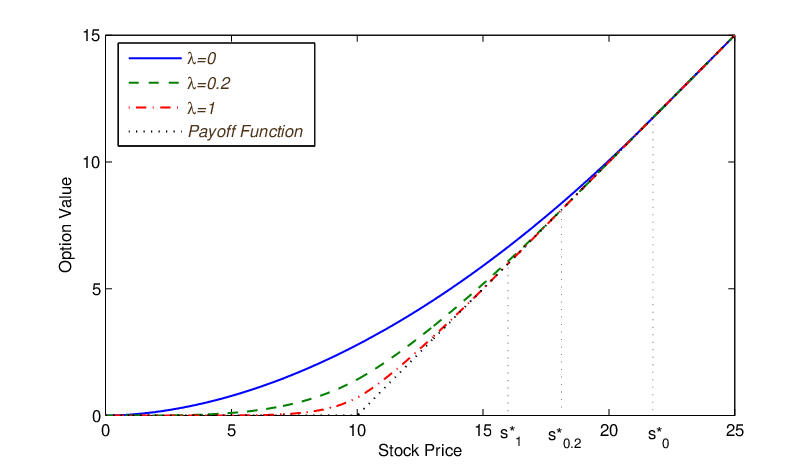
When a vesting period of years is imposed, we compute the ESO cost at time from the conditional expectation
| (6.10) |
By substituting the vested ESO cost function into (6.10), and recognizing that , for any , is lognormal, we can directly compute the unvested ESO cost.
Corollary 6.2
Under the GBM model, the unvested perpetual ESO cost admits the formula
| (6.11) | ||||
where is the standard normal complementary c.d.f. and
| (6.12) | ||||
| (6.13) | ||||
| (6.14) |
In contrast to its vested counterpart, the unvested ESO cost is time-dependent. In Figure 7 (left), we observe that the perpetual ESO cost decreases as the vesting period increases. A higher job termination rate not only decreases the ESO cost (see Figure 6) but also the exercise threshold (see Figure 7 (right).


7 Conclusions
We have provided the analytical and numerical studies for the valuation and risk analysis of ESOs under Lévy price dynamics. Our results are useful for reporting ESO cost, as mandated by regulators, and for understanding holder’s exercise behavior. In particular, we show job termination risk has a direct effect on the ESO holder’s exercise timing, which in turn affects the ESO cost as well as contract termination probability. For future research, risk estimation for large ESO portfolios is both practical and challenging. Other related issues include the incentive effect and optimal design of ESOs and other compensation schemes, such as restricted stocks. Lastly, our valuation framework can also be applied to pricing American options with liquidity, default, or other event risks. This would require an appropriate modification of the payoff at the exogenous termination time.
Appendix A Appendix
A.1 Proof of Proposition 2.1
Let and be the vested ESO cost associated with and , respectively, and assume . We define an operator by
| (A.1) |
From the variational inequality (2.12), we see that . We choose a point in the continuation region of , which means that . Since and , direct substitution shows that .
Next, we define the process
| (A.2) |
Using the fact that and Optional Sampling Theorem, we deduce that, for any ,
| (A.3) |
In particular, we denote and as the optimal stopping times associated with and , and get
| (A.4) | ||||
| (A.5) | ||||
| (A.6) |
The last inequality follows since is one candidate stopping time for the optimal stopping value function . Hence, we conclude that . This implies that any point in the continuation region of must also lies in the continuation region of , which means that the optimal exercise boundary for dominates that for .
As for the unvested ESO, the job termination intensity reduces its terminal values, and increases the probability of forfeiture (with payoff zero) during the vesting period. As a result, a higher job termination intensity also reduces the unvested ESO cost.
A.2 Proof of Proposition 6.1
We conjecture that it is optimal to exercise the ESO as soon as the stock reaches some level . Then, we split the stock price domain into three regions: , , and . In region 1, we have and . In region 2, the ESO cost solves the inhomogeneous ODE
| (A.7) |
One can check by substitution that the general solution to (A.7) is given by
| (A.8) |
where and are given in (6.4).
In region 3, since the option is out of the money, we have the ODE
| (A.9) |
whose solution is the form . Since as , it follows that .
To solve for the constants , along with the critical stock price , we apply continuity and smooth-pasting conditions at and to get
| (A.10) | ||||
| (A.11) | ||||
| (A.12) | ||||
| (A.13) |
Solving this system of equations yields (6.5)-(6.6). In particular, we see that since and .
From (A.12)-(A.13), the threshold satisfies the equation
| (A.14) |
To show this has a unique real solution, we note that is continuous, and
| (A.15) |
since , and . In addition, we have the limits: and , as well as . Together, this implies has a unique real root . Hence, we obtain formula (6.3) for . By direct substitution, it satisfies the VI (6.2).
A.3 Finite Difference Method for ESO Valuation
We summarize the finite difference method (FDM) for computing the ESO costs in Tables 3 and 5. For this purpose, we adapt the FDM algorithm for European options detailed in Cont and Voltchkova (2003) to the current case of early exercisable ESO with job termination risk.
First, we introduce the change of variable and denote . Then, the PIDE for the vested ESO cost in the continuation region becomes
| (A.16) |
for , with the initial condition , where
| (A.17) |
To proceed, we split the operator into two parts, namely,
| (A.18) |
where
| (A.19) |
with .
We define a uniform grid on by , with . In Tables 3 and 5, we have and . Also, denote be the cost at the grid point . We use trapezoidal quadrature rule with to approximate the integral terms in (A.19). To do so, we let , be such that , and apply the approximations
with
The space derivatives are approximated by the finite differences
| (A.20) |
Next, we replace and with their approximations and , respectively. Lastly, we arrive at the following implicit-explicit time-stepping scheme:
| (A.21) |
where
| (A.22) |
Due to the early exercise feature, the iteration is coupled with a comparison to the payoff from immediate exercise. After computing the vested ESO cost till the end of the vesting period, similar finite difference method can be applied to solve the PIDE for the unvested ESO cost:
| (A.23) |
for .
The above algorithm works for the case when the underlying Lévy process has finite activity, with . In the infinite activity case with , we we can use an auxiliary process with the Lévy triplet to approximate the original process , where and is again determined by the risk-neutral condition. Therefore, satisfies
| (A.24) |
for with initial condition . Here, the operator is defined by
| (A.25) |
with
The PIDE in (A.24) can be solved by the same numerical scheme as in the finite activity case. We apply this finite difference method for comparing with our FST method. For alternative finite difference methods, especially those designed to address specific Lévy processes, such as VG and CGMY, we refer to Hirsa and Madan (2004), Forsyth et al. (2007), and references therein.
A.4 Closed-Form Probabilities
The probability that an ESO cost surpasses a given threshold , as defined in (5.3), can be viewed as a European digital option with zero interest rate, computed under . We summarize the corresponding closed-form formulas under the GBM, Merton, and Kou models (see Table 2).
(i) Under the GBM model, the ESO cost exceedance probability is given by
| (A.26) |
and is the standard normal c.d.f.
(ii) When the company stock price follows the Merton jump diffusion, we have
| (A.27) |
(iii) In the Kou jump diffusion model, the probability of cost exceedance is given by
| (A.28) |
where
with , and .
References
- Bayraktar and Xing (2009) Bayraktar, E. and Xing, H. (2009). Analysis of the optimal exercise boundary of American options for jump diffusions. SIAM Journal on Mathematical Analysis, 41:825–860.
- Bettis et al. (2005) Bettis, J. C., Bizjak, J. M., and Lemmon, M. L. (2005). Exercise behaviors, valuation, and the incentive effects of employee stock options. Journal of Financial Economics, 76(2):445–470.
- Black and Scholes (1973) Black, F. and Scholes, M. (1973). The pricing of options and corporate liabilities. Journal of Political Economy, 3:637–654.
- Carpenter et al. (2010) Carpenter, J., Stanton, R., and Wallace, N. (2010). Optimal exercise of executive stock options and implications for firm cost. Journal of Financial Economics, 98(2):315–337.
- Carr (1998) Carr, P. (1998). Randomization and the American put. Review of Financial Studies, 11:597–626.
- Carr et al. (2002) Carr, P., Geman, H., Madan, D. B., and Yor, M. (2002). The fine structure of asset returns: An empirical investigation. Journal of Business, 75(2):305–332.
- Carr and Linetsky (2000) Carr, P. and Linetsky, V. (2000). The valuation of executive stock options in an intensity-based framework. European Finance Review, 4(2):211–230.
- Carr and Madan (1999) Carr, P. and Madan, D. B. (1999). Option pricing using the fast Fourier transform. Journal of Computational Finance, 2(1):61–73.
- Chance and Yang (2005) Chance, D. and Yang, T.-H. (2005). The utility-based valuation and cost of executive stock options in a binomial framework: Issues and methodologies. Journal of Derivatives Accounting, 2(2):165–188.
- Cont and Voltchkova (2003) Cont, R. and Voltchkova, E. (2003). A finite difference scheme for option pricing in jump-diffusion and exponential Lévy models. SIAM Journal on Numerical Analysis, 43(4):1596–1626.
- Cvitanić et al. (2008) Cvitanić, J., Wiener, Z., and Zapatero, F. (2008). Analytic pricing of employee stock options. Review of Financial Studies, 21(2):683–724.
- d’Halluin et al. (2003) d’Halluin, Y., Forsyth, P., and Labahn, G. (2003). A penalty method for American options with jump diffusion processes. Numerische Mathematik, 97(2):321–352.
- Forsyth et al. (2007) Forsyth, P. A., Wang, I. R., and Wan, J. W. (2007). Robust numerical valuation of European and American options under the CGMY process. Journal of Computational Finance, 10(4):31–69.
- Frydman and Jenter (2010) Frydman, C. and Jenter, D. (2010). CEO Compensation. Annual Review of Financial Economics, 2(1):75–102.
- Grasselli and Henderson (2009) Grasselli, M. and Henderson, V. (2009). Risk aversion and block exercise of executive stock options. Journal of Economic Dynamics and Control, 33(1):109–127.
- Hirsa and Madan (2004) Hirsa, A. and Madan, D. (2004). Pricing American options under Variance Gamma. Journal of Computational Finance, 7(2):63–80.
- Huddart (1994) Huddart, S. (1994). Employee stock options. Journal of Accounting and Economics, 18(2):207–231.
- Huddart and Lang (1996) Huddart, S. and Lang, M. (1996). Employee stock option exercises: an empirical analysis. Journal of Accounting and Economics, 21:5–43.
- Hull and White (2004) Hull, J. and White, A. (2004). How to value employee stock options. Financial Analysts Journal, 60(1):114–119.
- Jackson et al. (2008) Jackson, K. R., Jaimungal, S., and Surkov, V. (2008). Fourier space time-stepping for option pricing with Lévy models. Journal of Computational Finance, 12(2):1–29.
- Jennergren and Naslund (1993) Jennergren, L. and Naslund, B. (1993). A comment on ‘Valuation of stock options and the FASB proposal’. Accounting Review, 68(1):179–183.
- Kou (2002) Kou, S. G. (2002). A jump-diffusion model for option pricing. Management Science, 48(8):1086–1101.
- Kyprianou and Pistorius (2003) Kyprianou, A. E. and Pistorius, M. R. (2003). Perpetual options and Canadization through fluctuation theory. Annals of Applied Probability, 13(3):1077–1098.
- Lamberton and Mikou (2008) Lamberton, D. and Mikou, M. (2008). The critical price for the American put in an exponential Lévy model. Finance and Stochastics, 12(4):561–581.
- Leung and Sircar (2009) Leung, T. and Sircar, R. (2009). Accounting for risk aversion, vesting, job termination risk and multiple exercises in valuation of employee stock options. Mathematical Finance, 19(1):99–128.
- Lord et al. (2008) Lord, R., Fang, F., Bervoets, F., and Oosterlee, K. (2008). A fast and accurate FFT based method for pricing early-exercise options under Lévy processes. SIAM Journal on Scientific Computing, 30(4):1678–1705.
- Madan et al. (1998) Madan, D. B., Carr, P., and Chang, E. (1998). The Variance Gamma process and option pricing. European Finance Review, 2(8):79–105.
- Marquardt (2002) Marquardt, C. A. (2002). The cost of employee stock option grants: An empirical analysis. Journal of Financial Economics, 40(4):1191–1217.
- McDonald and Siegel (1986) McDonald, R. and Siegel, D. (1986). The value of waiting to invest. Quarterly Journal of Economics, 101:707–727.
- McKean (1965) McKean, H. P. J. (1965). Appendix: A free boundary problem for the heating function arising from a problem in mathematical economics. Industrial Management Review, 6:32–39.
- Merton (1976) Merton, R. (1976). Option pricing when underlying stock returns are discontinuous. Journal of Financial Economics, 3:125–144.
- Pham (1997) Pham, H. (1997). Optimal stopping, free boundary, and American option in a jump diffusion model. Applied Mathematics and Optimization, 35(2):145–164.
- Samuelson (1965) Samuelson, P. (1965). Rational theory of warrant pricing. Industrial Management Review, 6:13–31.
- Sato (1999) Sato, K.-I. (1999). Lévy Processes and Infinitely Divisible Distributions. Cambridge Studies in Advanced Mathematics. Cambride University Press.
- Szimayer (2004) Szimayer, A. (2004). A reduced form model for ESO valuation: Modelling the effects of employee departure and takeovers on the value of employee share options. Mathematical Methods of Operations Research, 59(1):111–128.