Overcoming erasure errors with multilevel systems
Abstract
We investigate the usage of highly efficient error correcting codes of multilevel systems to protect encoded quantum information from erasure errors and implementation to repetitively correct these errors. Our scheme makes use of quantum polynomial codes to encode quantum information and generalizes teleportation based error correction for multilevel systems to correct photon losses and operation errors in a fault-tolerant manner. We discuss the application of quantum polynomial codes to one-way quantum repeaters. For various types of operation errors, we identify different parameter regions where quantum polynomial codes can achieve a superior performance compared to qubit based quantum parity codes.
December 2016
1 Introduction
A quantum erasure channel replaces a qubit (qudit) with an “erasure state” that is orthogonal to all the basis states of a qubit (qudit) with a certain probability, thereby erasing the qubit (qudit) and enabling the receiver know that it has been erased [1]. Physically, erasure errors may occur in various situations, such as leakage to other states [2, 3, 4], atom losses [5], and photon losses [6, 7, 8, 9]. For ion-trap systems, leakage processes occur when the qubit moves out of the idealized two-level sub-space to a larger space [2, 3, 4]. For quantum memories with optical lattices, back ground gas collisions can eject the atoms leading to atom losses [5] Photon losses occur in linear optical quantum computing schemes [6] due to absorption in optical interconnects or optical fiber. Undoubtedly, protecting quantum information from erasure errors is a significant challenge for practical quantum computation and long distance quantum communication.
Specifically, for long distance quantum communiction through optical fibers, photon losses lead to an exponential penality in resources and time. The exponential penality can be overcome by establishing intermediate repeater stations and actively correcting for erasure and operation errors at these stations. Three generations of quantum repeaters have been proposed based on the different approaches used to correct erasure and operation errors [10]. The first generation employs heralded entanglement generation between neighboring repeater stations to correct erasure errors and entanglement purification to correct operation errors [11]. Heralded entanglement generation needs two-way classical communication between neighboring repeater stations, while entanglement purification needs two-way classical communication between remote repeater stations. The second generation [12, 13, 14, 15] employs heralded entanglement generation to correct erasure errors and quantum error correction to correct operation errors. Quantum error correction doesn’t require any form of two-way classical communication. The third generation uses quantum error correction to correct both loss and operation errors, and avoids any form of two-way classical communication between repeater stations, thereby rendering ultrafast communication over transcontinental distances [16, 17, 18, 19, 20, 21]. Since erasure errors are actively corrected in these repeater schemes, it is crucial to investigate quantum error correcting codes that can correct erasure errors very efficiently [22, 23, 24, 25]. So, far only quantum parity codes (QPC) have been optimized for third generation quantum repeaters [26, 17].
Due to the quantum no-cloning theorem [1], no error correcting code can correct erasure errors deterministically when the erasure rate is above . There have been significant advances in searching for quantum codes that can correct up to erasure error rates. Varnava et. al. [22] showed that by using tree-like cluster states for encoding, one can correct erasure errors when erasure rate is close to the bound for one-way quantum computation. Stace and Barrett [24, 23] demonstrated that surface codes can also correct erasure errors when error rates are close to . However, qubit based codes often require large code size to enable the correction of a large fraction of erasure errors.
Quantum error correcting codes of higher-dimensional systems provide a promising alternative to qubit based encoding schemes to correct erasure errors. For example, quantum polynomial codes (QPyC) [27, 28] are a class of CSS codes that were introduced in the context of fault-tolerant quantum computation [27] and shown to be useful for constructing threshold quantum secret sharing schemes [28]. One can encode a secret qudit into qudits (with prime dimension ) and distribute one qudit to each of the many parties, so that at least of them should get together to reconstruct the secret. This makes the QPyC a good choice for the correction of erasure errors up to a fraction of for a large .
This paper is organized as follows: We first perform a comparison between code and the code. In section III, we investigate the ability of general QPyC to correct erasure errors and compare them to surface codes. In section IV, we show that QPyC can be used for third generation (or one-way) quantum repeaters. We also compare our quantum repeater scheme with other schemes based on quantum parity codes [26, 17] in the presence of operation errors. Here, we identify the parameter regimes where QPyC performs better than QPC. The price for this improved performance against erasure errors is that more complex multi-mode operations must be implemented for encoding and readout operations. In section V, we discuss the key experimental techniques needed for the physical implementation of our scheme and provide potential experimental procedures based on atom mediated photonic gates for multilevel systems.
2 Three-qutrit code vs Four-qubit code
To illustrate how the error correction for erasure errors works, consider the four-photon code that maps two qubits into the logical states [25, 29],
| (1) | |||||
where the subscripts 1-4 denote qubits 1-4. Here, and corresponds to a single photon occupying two different modes such as polarization or time-bin states ’01’ and ’10’ respectively. The [[4,2,2]] code requires a total of four pairs of modes (eight modes) and four photons. The loss of a photon leads to the vacuum state of the associated pair of modes, which corresponds to an erasure error. Suppose we transmit the encoded state through a channel and it undergoes one photon loss (i. e. erasure of one of qubits), then the quantum error correcting code enables the reconstruction of the encoded state as follows. First, we use quantum non-demolition measurement to extract the total excitation number for each pair of modes (without destroying the qubit), which will be one if there is no photon loss, or zero if the photon is lost. Hence, the photon loss can be identified as an erasure error of the associated qubit. For example, if the first qubit is erased, to reconstruct the encoded state we apply two CNOT gates betweeen qubits 3 and 2, and qubits 4 and 2 respectively. Then, we measure qubit 2 in the Z basis and and use the measurement outcome to reconstruct the logical state. This can be seen by studying the logical operators of the code, , , and . After the CNOT gates, the logical operators are transformed into , , and respectively. After the gates, a Z-measurement on the second qubit is needed to decode the code. We refer the readers to Ref. [25], where an alternative non-destructive method has been proposed to recover the logical qubits. It has been proven that we need at least four qubits to correct one erasure error [30].
Alternatively, one can also correct an erasure error using a code which encodes a logical qutrit into three physical qutrits as [28],
| (2) | |||||
where the subscripts 1-3 represent qutrits 1-3. Here, we note that each qutrit represents different time bin states and not photon number. More specifically, , and represent temporal modes ’001’, ’010’ and ’100’ respectively. So, the code requires a total of three triplets of modes (nine modes) and three photons. Photon loss leads to the vacuum state of the corresponding triplet of modes, which can identified as the erasure error of the associated qutrit. If qutrit is erased, it is possible to reconstruct the encoded qutrit by performing an addition modulo 3 operation between the other two qutrits. For example, for the incoming state , if the first qutrit is erased, then the state of second and third qutrits is given by
| (3) | ||||
| where, | ||||
Using two addition modulo 3 operations11 1 An addition modulo 3 operation refers to a SUM gate here is described in detail in the section IV. between qutrits 2 and 3, and then between qutrits 3 and 2, we can reconstruct the encoded state.
We now compare the code and the code for different loss rate per photon, . Since each logical qutrit can carry qubits of information, we multiply a factor of when computing bits/photon and bits/mode for code. As illustrated in Fig. 1, the bits/photon is always higher for the code compared to the code for all loss rates . With regard to the bits/mode, for large loss rates , the code performs better than the code. In principle, by concatenating the code, it is possible to supress more erasure errors. However, to be resource efficient we will consider the generalization of the codes - QPyC in the forthcoming section.
3 Quantum Polynomial codes
The qutrit code can be generalized to -level ( is a prime number) qudit system as a code, which encodes one logical qudit into physical qudits and can correct up to erasure errors [28]. The QPyC code is a CSS code which can be obtained from classical polynomial code. The encoded states of the QPyC code are given by [27, 28],
| (4) |
Here, labels the logical states with . The labels ,,…, are distinct elements of F, where . is the first prime number that is no less than . The polynomial is given by with . For , , it can be seen that
| (5) |
yielding the code (see Eq. (2)). The success probability of recovering the encoded quantum information after it has undergone erasure errors is given by
| (6) |
Note that for a reasonable code size, it is possible to achieve substantially low (e. g. ) failure rate even in the presence of high erasure rate . Note that with about 40 qudits one can suppress the failure rate to for erasure rate.
It can be seen from Eq. (6) that at , independent of the code size. Further, note that the success probability of error correction has a phase transition behaviour with , for and for . One can obtain the critical exponent of phase transition by noting that for , around the fixed point , the asymptotic expression is
| (10) |
For , making the approximation that , and , then
| (11) |
That means for given ,
| (12) |
yielding a critical exponent of 2.
We will now compare the performance of QPyC with surface codes [24] for the correction of erasure errors. Surface codes consists of a square lattice with qubits in total, where each qubit located on the edges of the square lattice. The logical operators () of the surface codes are given by the product of () operators along a non-trivial homological cycle connecting the boundaries [24]. Therefore, the success probability of bond percolation in the square lattice and its dual lattice [22] is essentially the same as the probability of decoding the surface code. It is well known that the bond percolation threshold is for a square lattice, meaning that as the distance of the lattice , for and for .
In Fig. 2 we study the success probabilities of surface codes with three different distances and find that at , , while in Fig. 2 we see that for all code sizes. Therefore, when is around , QPyC of any code size always outperforms surface codes. Further, it can be seen in Fig. 2 that threshold for surface codes with is about , and the threshold approaches for larger code sizes, while the threshold of QPyC is for all code sizes. In practice, we might operate the codes at a loss probability much lower than . Hence, we assume and compare the surface code and QPyC with so that they have a similar Hilbert space dimension for physical encoding. As illustrated in Table 1, for smaller code sizes surface codes performs better than QPyC and with and , QPyC outperforms surface codes with a smaller failure probability.
| Surface code | QPyC | ||
|---|---|---|---|
4 Application in quantum repeaters
One-way (or third generation) quantum repeaters [16, 17, 26, 31, 10] rely on quantum error correction to relay data from one repeater station to the next. At each station, error correction operations are performed before the message is transmitted to the next station. Recently, it has been shown that QPC [32, 17, 26] (a generalization of the code) can correct erasure errors efficiently by teleportation based error correction (TEC). Since QPyC corrects a larger fraction of erasure errors, it is reasonable to consider QPyC instead of QPC for one-way quantum repeaters, and expect a significant improvement for resource consumption and key generation rates.
4.1 Implementation of error correction for erasure errors
For qubit encoding schemes, it has been shown that TEC [33, 34] is an effective approach for the correction of erasure and operation errors. Since teleportation requires and measurements on qubits, error correction for erasure and operation errors is possible if we can reliably measure the logical operators and of the error correcting code [26]. For example, the code has stabilizers and and the following logical operators: , , and . If any qubit undergoes an erasure error, all the operators and operators can be measured in the TEC circuit and the encoded qubits can be retrieved. For example, if the first qubit is lost, one can calculate the operators , , and and retrive the encoded qubits. We generalize TEC to multilevel systems in Fig. 3 by using generalized Pauli matrices that act on -level system as and , [35] and SUM gate that acts on a control qudit with a target qudit to produce the transformation [35]. Consider the code with stabilizers , and operator that corresponds to one of the operators and operator that corresponds to one of the operators . It can be readily seen that in the presence of an erasure error on any qutrit one can still measure the corresponding logical operator and reconstruct the encoded state.
4.2 Error model for operation errors
Suppose that each physical qudit is encoded into a QPyC and is transmitted through repeater stations, where the TEC is implemented. We assume independent errors acting on physical qudits and consider an extensive error model with the following types of errors acting on the encoded qudit as follows:
- 1.
The photon arrives at each repeater station with probability , where is the repeater spacing and is the attenuation length of the fiber.
- 2.
The photon undergoes depolarization with a probability . For simplicity, we assume that this is also the probability of error on each physical qudit of the encoded Bell pair prepared at the repeater station.
- 3.
The photon experiences an additional dephasing in the matter qubit-photon coupling with a probability .
- 4.
Each SUM gate acting between the encoded Bell pair and the incoming qubit (see Fig. 3) fails at a probability .
By further assuming the same probabilities for all types of depolarization errors and gate errors, the transmission channel with the incoming single qudit state takes the form,
| (13) |
Similarly, the imperfect gate between the incoming qudit A and qudit B at repeater station can be modeled as
| (14) |
For each qudit the locally prepared logical states and , we assume it undergoes depolarization, which can be modelled as
| (15) |
In contrast to the error models in [26, 10], we track the errors in the preparation of the logical Bell state needed for TEC. From these error channels, we can calculate the probability of having an error in any one of the measurements up to the first order as
| (16) |
Once the encoded state is transmitted from one repeater station to its neighbor, there exists three possibilities at the receiving repeater station
- 1.
More than photons are lost in transit and the outcome of the measurement cannot be found leading to a heralded failure with probability .
- 2.
At least photons are received, but the encoded state is not decoded correctly due to the presence of many operation errors and the encoded state is not decoded correctly with probability .
- 3.
At least photons are received to make an encoded measurement and the encoded state is decoded correctly with probability .
The probability that a heralded failure does not happen at any one of the repeater stations is given by, . Let us suppose that photons are lost before the destination. Among the rest of the photons that reach the destination, photons suffer operation errors. As such, the code can correct up to errors. The probability of successfully measuring the encoded X/Z measurement outcomes is given by,
| (17) |
The probability of incorrect decoding of the qudit is given by,
| (18) |
It is easy to verify that . By making a pessimistic assumption that an effective logical error in any one of the repeater stations is an overall logical error at the receiver’s end, the logical error rate of the encoded quantum information can be defined conditioned on the success of receving enough photons as,
| (19) |
For the two basis protocol for quantum key distribution (where information is encoded in only two logical bases and ), the asymptotic normalized secure key generation rate is [36].
| (20) |
where is the time taken for local operations with
| (21) | |||||
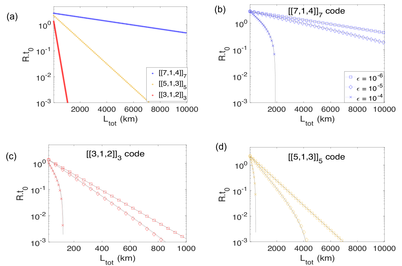
In Fig. 4(a), we study the dependence of the secure key generation rate , with respect to the total distance of communication for small encoded blocks of QPyC, assuming 1 km repeater spacing and no operation errors. For , 3 qudits are sufficient to reach 700 km with key generation rates 10kHz. We can increase the total range of communication to 10,000km by using 7 qudits and obtain a key generation rate 1000kHz. As the operation errors involved with the error correction increases, increases exponentially after a certain distance and we can expect a quick decay of over a certain . The maximum that the QPyC can tolerate depends on the dimension of the code. We can check that for the code, code and codes respectively for the codes to yield non zero key generation rates. Taking only the leading terms into account in Eq. (17), we can approximate for the code, for the code and for the code respectively. Further, since for 1km spacing is negligible, we should have , yielding
| (22) |
For example, for , = 1km, we get for , and codes respectively as confirmed by the ”” lines in Fig. (4). In Fig. 4(b-d), we study the variation of for varying operation errors for , and codes respectively. We fit the points obtained from a rigorous theoretical calculation with the approximate mentioned above (shown as gray curve in Fig. 4) and observe a good match between them.
4.3 Comparison with QPC
We can compare the performance of different quantum codes for one-way quantum repeaters by considering both the qubit and temporal resources consumed by the code, respectively. In order to compare QPyC codes, which use multilevel systems, with QPC of qubits, we consider the conversion of a -level qudit into qubits and compare the performance of the codes by a cost coefficient [26]
| (23) |
The is obtained from the product of qubit resources and temporal resources. The number of qubits used for TEC at every repeater station is given by and the number of qubits for all stations is . The temporal resource used by the scheme is simply the inverse of key generation rate, i.e. . Since, the product of qubit and temporal resources varies at least linearly with , we further divide the product by to obtain the cost coefficient, which stands for the number of qubits required per km for the generation of one secure bit in one second.
We find that the present scheme with QPyC can achieve a very small cost coefficient, which is about 5 times less than for QPC with TEC for km in the absence of operation errors. Note that in addition to the local resource overhead, we can also save the number of modes considerably by using QPyC instead of QPC (See Appendix A). In the presence of operation errors, the comparison between qubit and qudit based schemes for QRs depends largely on the error model because of the complexity involved in the implementation of multimode operations. Although it is challenging to compare the resource requirements between these codes, we have attempted to ensure a fair comparison by assuming that the operation errors increase with dimension of the qudit. We assume that , , and for the comparison. In Fig. 5, we investigate the variation of the ratio of cost coefficients with respect to total distance of communication . We consider only one of the errors , and respectively in each one of the plots and show the variation of the ratio of the cost coefficients with respect to and the corresponding picked by the optimization of the cost coefficient shown in the colored contour. As the operation error increases, the ratio decreases and QPC becomes more favorable than QPyC shown in the area above the break-even contour line (shown as thickened line) as the number of levels increases. Since scales as and , the optimization is forced to choose a smaller code for large total distances in Fig. 5(a) compared to Fig. 5(b) and Fig. 5(c).

5 Physical implementation
For the implementation of quantum repeaters with QPyC encoding schemes, we can consider time-bin photonic qudits. The time-bin qudit has a single photon excitation in a superposition of time-bins, which can be efficiently generated at telecom wavelengths and coupled into an optical fiber [37]. The TEC circuit, which is essential of our scheme, requires single qudit - and -operation, two-qudit SUM gate, - and -measurement of qudits. The SUM gate can be further decomposed using Controlled Z (CZ) gate and Fourier gates [35].
For the time-bin qudits, the -operation and Z-measurement can be implemented by a selectively phase shifting or detection at different time slots. -operation and -measurement can be achieved by making a strong dispersive medium that interferes different time-bins as detailed below. For the two-qudit gate, the direct photon-photon interaction is negligible due to weak single photon nonlinearity. Therefore, we propose to use a nanophotonic-atom interference to store and manipulate the photonic qudits and to mediate photon-photon qudits gate.
The feasible experimental system adapted from Ref. [38] is illustrated in Fig. 6(a). A single atom is trapped in the vicinity of a fiber integrated photonic crystal nanocavity, single photons can be efficiently coupled to the nanocavity using the tapered fiber, which strongly interacts with the atom due to the very small mode volume of the nanocavity.
Based on the nanophotonic atom interface, we can implement the Fourier () [35] and -gates of single time-bin qudit by downloading the photonic time-bin qudit to the atom, and using photonic-atomic qudit control phase (CZ) gate. Based on these elementary gates, the -measurement can be realized by the combination of -gate and -measurement. The photon-photon qudit SUM gate can be realized by a sequence of Fourier gate on photon qudits and two CZ gates between photon and atom. In the following, we provide the details about experimental implementation of the above element gates: (1) and gate of single qudit, (2) the photon-atom qudit CZ gate, (3) the atom mediated photon-photon gates between time-bin qudits. Based on these three building blocks, QPyC can be corrected for erasure and operation errors using TEC and retransmitted to the neighboring station.
To illustrate the procedure, we consider the simplest case of qutrits. We choose the lines of natural atoms [39], with the transitions between hyperfine levels and . In addition, we use the as an ancillary state for processing the photonic qutrit. As illustrated in Fig. 6(b), we apply a tunable external magnetic field to introduce a relative frequency shift depending on hyperfine levels, which will be useful for the atom-photon coupling gate.
5.1 Single qudit and gates
Since it is difficult to make an -measurement on a time-bin photonic qutrit, we propose to transfer the quantum state from the time-bin photonic qutrit to either a multilevel atom or multiple two-level atoms. First of all, with microwave driving of transitions between F=1 and F=2 levels and also optical pumping, the single atom can be initialized to the ancillary state. Then, for single photon input to the cavity, it will be largely detuned from the transitions of the atoms. By applying an external laser driving with frequency , where is the energy difference between and , through a stimulated Raman adiabatic passage [40], the population will be transferred to if there is a single photon in the incoming time-bin, as shown in Fig. 6(b). By a sequence of microwave pulses, the population will be mapped to according to the order of input time-bin. This process effectively maps the state of the time-bin qutrit to the atom’s ground state levels. After that, we can carry out an -measurement by performing a Fourier transformation followed by a measurement on the atom. Alternatively, it is also possible to store the time-bin qutrit into multiple atoms and control the process by synchronized pulse sequences on individual atoms.
This procedure can be generalized to time-bin qudits in a straightforward fashion.

When the time-bin qudits are stored in atoms, arbitrary single qudit operations can be realized by applying either optical or microwave pulses. In the most general case, arbitrary unitary on single level system can be constructed by a series of gates between any two of levels (called Givens rotations) [41]. Alternatively, the arbitrary unitary can be realized with optimal controlled pulse sequences. For the qutrit case, there are more efficient schemes that only requires three steps, by either three Givens rotation or three Houlsehould’s reflections [42]. Recently, arbitrary unitary on hyperfine energy levels of atom has been demonstrated [43]. Two-qudit gates between atoms can be mediated by cavity photons. Generalization of such techniques [42] will enable the generation of the encoded Bell states needed for the TEC at repeater stations.
5.2 Controlled-Z gate between photonic and atomic qudits
To realize CZ gate between the time-bin photonic qutrit and the atom, we prepare the atom in the superposition of . Due to the strong cooperative interaction between the atom and nanocavity photon, the incoming single photon pulse input to the system have the reflectivity as [38]
| (24) |
where is the atom-photon interaction cooperativity, is the frequency detuning between the pulse and atomic transition frequency and is the excited state decay rate. For a large , and . Due to the magnetic field, the photon detuning for different gradually reduces with , corresponding to a atomic state dependent phase shift as shown in Fig. 6(c).
The CZ gate can be represented as , where denoting the states of photonic qutrits and is photon state dependent phase gate. The gate can be realized by the following three steps:
- 1.
For the first incoming pulse, all energy levels are detuned from the cavity mode by controlling external bias magnetic field such that then we have an operation on the atomic energy levels as
- 2.
For the second pulse, magnetic field is tuned to have , and , so that the phase shift is , and ,
- 3.
For the third pulse, the magnetic field is reversed, so that the phase shift is , and , then
The generalization of the CZ gate to higher dimensional qudits is less straightforward compared to time-bin storage. One possible realization is using the cavity coupled multiple -type atoms (each atom is an effective two-level system). Suppose there are atoms and each has ground states , and excited state , the transition is near resonance with cavity while is far off-resonance. In addition, the transition frequencies of atoms can be controlled by external electric or magnetic field individually. First, the atoms are initialized to , and transition frequencies are on-resonance with cavity. By single photon Raman transition of the atom ensemble, the states of atoms are prepared to the one-excitation Dicke state . Then, the CZ gate of -level time-bin qudit can be realized by shifting the transition frequencies of individual atoms: for -th () pulse input to the system, the -th () atom is tuned to be near-resonance on the cavity so that the reflected pulse gains a phase of .
5.3 Controlled-Z gate between time-bin qudits
A CZ gate can be realized between two physical time-bin photonic qudits by a generalization of the Duan-Kimble scheme [7]. The CZ gate between two time-bin photonic qutrits ( and ) can be realized by preparing the atomic state in a equal superposition of all energy levels and applying three photon-atom CZ gates ( with denoting the states of photonic qutrits) and two Fourier gates () on atoms as [27]
| (25) |
where,
| (26) |
The atomic state initialization and Fourier gates of atoms can be realized by microwave or optical Raman pulsed controlled transitions ( and ) and phase gate .
For qudits with , the Fourier gate of atoms can be realized by virtual cavity photon mediated atom-atom interaction, where strong pumping is applied on the transition, with the detuning equals to that between cavity photon and . Based on this procedure and the CZ gate between photonic and atomic qudits described in the previous section, the CZ gate between two time-bin qudits can be realized using a similar technique as Eq. (25).
6 Conclusion
We have investigated efficient codes using multilevel systems that can correct up to erasure error rates, which is the bound set by the no-cloning theorem [1]. The success probability of quantum polynomial codes close to erasure rates is higher than the success probability of surface codes of all code sizes. We employed teleportation based error correction that can correct erasure errors up to the threshold efficiently and discussed its application for the construction of highly efficient one-way quantum repeater networks. In comparison with quantum parity codes, we have obtained an improvement in resources by about 5 times for communication across 10,000km in the absence of operation errors and numerically identified the parameter regime, where the quantum polynomial codes perform better than quantum parity codes in the presence of operation errors. We have discussed the physical implementation of quantum polynomial codes and identified the key technological requirements. It will also be interesting to consider the experimental implementation of multilevel systems using oscillators [44], Rydberg atoms [45] and ensembles of multilevel systems [46]. Moreover, we can extend the coding schemes to continuous variables for the correction of erasure errors [47, 48]. Besides quantum communication, quantum error correcting codes for multilevel systems that can correct a large fraction of erasure errors might be useful for improving precision metrology [49, 50, 51, 52, 53].
Acknowledgements
This work was supported by the DARPA (Quiness program), ARL CDQI, NBRPC (973 program), Packard Foundation, Alfred P. Sloan Foundation, ARO (W911NF-14-1-0011, W911NF-14-1-0563), ARO MURI (W911NF-16-1-0349), NSF (EFMA-1640959), AFOSR MURI (FA9550-14-1-0052, FA9550-15-1-0015). We thank Siddharth Prabhu, Anup Rao, Victor Albert, Jungsang Kim, Norbert Lütkenhaus, Mikhail Lukin, Hong Tang and Steven Girvin for discussions.
APPENDIX A
In the manuscript, we have assumed that we are only limited by the qubit resources rather than the optical modes of the fiber channel. If qubit resource is no longer the limiting factor for one-way quantum repeaters, we should then compare the number of modes needed for different repeater schemes. For quantum state transfer using time-bin qudits, each qudit needs temporal modes for transmission. Therefore, the cost coefficient based on the number of modes for the transmission of photons is given by,
| (27) |
In Fig. 7, we compare the cost coefficients of QPyC and QPC. For QPC, since each qubit needs two temporal modes for transmission the numerical values of and are the same. For QPyC, the numerical value of is increased by a small factor compared to . We find that for km, QPyC achieves a cost that is about 3 times less than QPC.
References
- [1] Bennett C H, DiVincenzo D P and Smolin J A 1997 Phys. Rev. Lett. 78 3217
- [2] Preskill J 1998 Proc. Roy. Soc. London 454 385 http://rspa.royalsocietypublishing.org/cgi/doi/10.1098/rspa.1998.0167
- [3] Wu L A, Byrd M S and Lidar D A 2002 Phys. Rev. Lett. 89 127901 http://link.aps.org/doi/10.1103/PhysRevLett.89.127901
- [4] Fazio R, Palma G M and Siewert J 1999 Phys. Rev. Lett. 83 5385 http://link.aps.org/doi/10.1103/PhysRevLett.83.5385
- [5] Vala J, Whaley K B and Weiss D S 2005 Phys. Rev. A 72 052318 http://link.aps.org/doi/10.1103/PhysRevA.72.052318
- [6] Knill E, Laflamme R and Milburn G J 2001 Nature (London) 409 46 http://www.ncbi.nlm.nih.gov/pubmed/11343107
- [7] Duan L M and Kimble H J 2004 Phys. Rev. Lett. 92 127902 http://link.aps.org/doi/10.1103/PhysRevLett.92.127902
- [8] Kok P, Munro W J, Nemoto K, Ralph T C, Dowling J P and Milburn G J 2007 Rev. Mod. Phys. 79 135 http://link.aps.org/doi/10.1103/RevModPhys.79.135
- [9] Bell B A, Herrera-Martí D A, Tame M S, Markham D, Wadsworth W J and Rarity J G 2014 Nature Comm. 5 3658 http://www.ncbi.nlm.nih.gov/pubmed/24752224http://www.nature.com/doifinder/10.1038/ncomms4658
- [10] Muralidharan S, Li L, Kim J, Lütkenhaus N, Lukin M D and Jiang L 2016 Scientific Reports 6 20463
- [11] Briegel H J, Dur W, Cirac J I and Zoller P 1998 Phys. Rev. Lett. 81 5932
- [12] Jiang L, Taylor J M, Nemoto K, Munro W J, Van Meter R and Lukin M D 2009 Phys. Rev. A 79 32325
- [13] Bratzik S, Kampermann H and Bruss D 2014 Phys. Rev. A 89 32335
- [14] Epping M, Kampermann H and Bruß D 2016 Applied Physics B: Lasers and Optics 122 54
- [15] Pant M, Krovi H, Englund D and Guha S 2016 arxiv: quantph:/1603.01353
- [16] Fowler A G, Wang D S, Hill C D, Ladd T D, Van Meter R and Hollenberg L C L 2010 Phys. Rev. Lett. 104 180503
- [17] Munro W J, Stephens A M, Devitt S J, Harrison K A and Nemoto K 2012 Nature Phot. 6 777
- [18] Muralidharan S, Kim J, Lütkenhaus N, Lukin M D and Jiang L 2014 Phys. Rev. Lett. 112 250501
- [19] Ewert F, Bergmann M and van Loock P 2016 Phys. Rev. Lett. 117 210501
- [20] Namiki R, Jiang L, Kim J and Lütkenhaus N 2016 Phys. Rev. A 94 052304
- [21] Glaudell A N, Waks E and Taylor J M 2016 New Jour. of Phys. 18 093008 http://stacks.iop.org/1367-2630/18/i=9/a=093008?key=crossref.532d612b4f9628dc8b5ec1c563c8ed3c
- [22] Varnava M, Browne D E and Rudolph T 2006 Phys. Rev. Lett. 97 120501 http://link.aps.org/doi/10.1103/PhysRevLett.97.120501
- [23] Barrett S D and Stace T M 2010 Phys. Rev. Lett. 105 200502 http://link.aps.org/doi/10.1103/PhysRevLett.105.200502
- [24] Stace T M and Barrett S D 2010 Phys. Rev. A 81 022317 http://link.aps.org/doi/10.1103/PhysRevA.81.022317
- [25] Gingrich R M, Kok P, Lee H, Vatan F and Dowling J P 2003 Phys. Rev. Lett. 91 217901 http://link.aps.org/doi/10.1103/PhysRevLett.91.217901
- [26] Muralidharan S, Kim J, Lütkenhaus N, Lukin M D and Jiang L 2014 Phys. Rev. Lett. 112 250501
- [27] Aharonov D and Ben-Or M 2008 SIAM J. Comput. 38 1207
- [28] Cleve R, Gottesman D and Lo H K 1999 Phys. Rev. Lett. 83 648 http://link.aps.org/doi/10.1103/PhysRevLett.83.648
- [29] Lu C Y, Gao W B, Zhang J, Zhou X Q, Yang T and Pan J W 2008 Proc. Natl. Acad. Sci. USA 105 11050 http://www.pubmedcentral.nih.gov/articlerender.fcgi?artid=2516277{&}tool=pmcentrez{&}rendertype=abstract
- [30] Grassl M, Beth T and Pellizzari T 1997 Phys. Rev. A 56 33 http://link.aps.org/doi/10.1103/PhysRevA.56.33
- [31] Zwerger M, Briegel H J and Dür W 2014 Sci. Rep. 4 5364
- [32] Ralph T C, Hayes A J F and Gilchrist A 2005 Phys. Rev. Lett. 95 100501 http://link.aps.org/doi/10.1103/PhysRevLett.95.100501
- [33] Knill E 2005 Phys. Rev. A 71 042322 http://link.aps.org/doi/10.1103/PhysRevA.71.042322
- [34] Knill E 2005 Nature (London) 434 39 http://www.ncbi.nlm.nih.gov/pubmed/15744292
- [35] Gottesman D 1999 Chaos, Solitons & Fract. 10 1749 http://linkinghub.elsevier.com/retrieve/pii/S0960077998002185
- [36] Sheridan L and Scarani V 2010 Phys. Rev. A 82 030301 http://link.aps.org/doi/10.1103/PhysRevA.82.030301
- [37] Marcikic I, De Riedmatten H, Tittel W, Zbinden H, Legré M and Gisin N 2004 Phys. Rev. Lett. 93 180502
- [38] Tiecke T G, Thompson J D, de Leon N P, Liu L R, Vuletic V and Lukin M D 2014 Nature(London) 508 241
- [39] Thompson J D, Tiecke T G, de Leon N P, Feist J, Akimov A V, Gullans M, Zibrov A S, Vuletić V and Lukin M D 2013 Science 340 1202 http://www.ncbi.nlm.nih.gov/pubmed/23618764
- [40] Bergmann K, Vitanov N V and Shore B W 2015 Jour. of Chem. Phys. 142 170901 http://dx.doi.org/10.1063/1.4916903
- [41] Bullock S S, O’Leary D P and Brennen G K 2005 Phys. Rev. Lett. 94 230502
- [42] Vitanov N V 2012 Phys. Rev. A 85 032331
- [43] Anderson B E, Sosa-Martinez H, Riofrío C A, Deutsch I H and Jessen P S 2015 Phys. Rev. Lett. 114 240401 http://link.aps.org/doi/10.1103/PhysRevLett.114.240401
- [44] Albert V V, Shu C, Krastanov S, Shen C, Liu R B, Yang Z B, Schoelkopf R J, Mirrahimi M, Devoret M H and Jiang L 2016 Phys. Rev. Lett. 116 140502
- [45] Rauschenbeutel A, Nogues G and Osnaghi S 2000 Science 288 2024 http://www.sciencemag.org/content/288/5473/2024.short
- [46] Brion E, Pedersen L H, Saffman M and Mølmer K 2008 Phys. Rev. Lett. 100 110506 http://link.aps.org/doi/10.1103/PhysRevLett.100.110506
- [47] Li L, Zou C L, Albert V V, Muralidharan S, Girvin S M and Jiang L 2016 arXiv:1609.06386v1 http://arxiv.org/abs/1609.06386
- [48] Bergmann M and Van Loock P 2016 Phys. Rev. A 94 012311
- [49] Kessler E M, Lovchinsky I, Sushkov A O and Lukin M D 2014 Phys. Rev. Lett. 112 150802 http://link.aps.org/doi/10.1103/PhysRevLett.112.150802
- [50] Arrad G, Vinkler Y, Aharonov D and Retzker A 2014 Phys. Rev. Lett. 112 150801 http://link.aps.org/doi/10.1103/PhysRevLett.112.150801
- [51] Dür W, Skotiniotis M, Fröwis F and Kraus B 2014 Phys. Rev. Lett. 112 080801 http://link.aps.org/doi/10.1103/PhysRevLett.112.080801
- [52] Preskill J 2000 arXiv:quant-ph/0010098 http://arxiv.org/abs/quant-ph/0010098
- [53] Macchiavello C, Huelga S F, Cirac J I, Ekert A K and Plenio M B 1998 Quantum Comm. Comput., and Measurement 337 http://link.springer.com/chapter/10.1007/0-306-47097-7{_}45