CERN-PH-TH-2015-097
Bootstrapping the Archipelago
Filip Kosa, David Polanda, David Simmons-Duffinb, Alessandro Vichic
a Department of Physics, Yale University, New Haven, CT 06520
b School of Natural Sciences, Institute for Advanced Study, Princeton, New Jersey 08540
c Theory Division, CERN, Geneva, Switzerland
Abstract
We study 3d CFTs with an global symmetry using the conformal bootstrap for a system of mixed correlators. Specifically, we consider all nonvanishing scalar four-point functions containing the lowest dimension vector and the lowest dimension singlet , assumed to be the only relevant operators in their symmetry representations. The constraints of crossing symmetry and unitarity for these four-point functions force the scaling dimensions to lie inside small islands. We also make rigorous determinations of current two-point functions in the and models, with applications to transport in condensed matter systems.
1 Introduction
Conformal field theories (CFTs) lie at the heart of theoretical physics, describing critical phenomena in statistical and condensed matter systems, quantum gravity via the AdS/CFT correspondence, and possible solutions to the hierarchy problem (and other puzzles) in physics beyond the standard model. Quite generally, they serve as the endpoints of renormalization group flows in quantum field theory. The conformal bootstrap [1, 2] aims to use general consistency conditions to map out and solve CFTs, even when they are strongly-coupled and do not have a useful Lagrangian description.
In recent years great progress has been made in the conformal bootstrap in , including rigorous bounds on operator dimensions and operator product expansion (OPE) coefficients [3, 4, 5, 6, 7, 8, 9, 10, 11, 12, 13, 14, 15, 16, 17, 18, 19, 20, 21, 22, 23, 24, 25, 26, 27, 28, 29, 30, 31, 32], analytical constraints [33, 34, 35, 36, 37, 38, 39, 40, 41, 42, 43, 44, 45], and methods for approximate direct solutions to the bootstrap [46, 47, 48, 49], including a precise determination of the low-lying spectrum in the 3d Ising model under the conjecture that the conformal central charge is minimized [50]. These results have come almost exclusively from analyzing 4-point correlation functions of identical operators. It is tantalizing that even more powerful constraints may come from mixed correlators.
In [51] some of the present authors demonstrated that semidefinite programming techniques can very generally be applied to systems of mixed correlators. In 3d CFTs with a symmetry, one relevant -odd operator , and one relevant -even operator , the mixed correlator bootstrap leads to a small and isolated allowed region in operator dimension space consistent with the known dimensions in the 3d Ising CFT. With the assistance of improved algorithms for high-precision semidefinite programming [52], this approach has culminated in the world’s most precise determinations of the leading operator dimensions in the 3d Ising CFT.
The immediate question is whether the same approach can be used to rigorously isolate and precisely determine spectra in the zoo of other known (and perhaps unknown) CFTs, particularly those with physical importance. In this work we focus on 3d CFTs with global symmetry, previously studied using numerical bootstrap techniques in [15, 22]. We will show that the CFTs known as the vector models can be similarly isolated using a system of mixed correlators containing the leading vector and singlet , assumed to be the only relevant operators in their symmetry representations.
We focus on the physically most interesting cases (e.g., see [53]) where the large- expansion fails. We do additional checks at . A summary of the constraints on the leading scaling dimensions found in this work are shown in figure 1. We also make precise determinations of the current central charge for . This coefficient is particularly interesting because it describes conductivity properties of materials in the vicinity of their critical point [54].
The 3d model (or model) has a beautiful experimental realization in superfluid 4He [55] which has yielded results for that are in tension with the leading Monte Carlo and high temperature expansion computations [56]. Our results are not yet precise enough to resolve this discrepancy, but we are optimistic that the approach we outline in this work will be able to do so in the near future. More generally, the results of this work give us hope that the same techniques can be used to to solve other interesting strongly-coupled CFTs, such as the 3d Gross-Neveu models, 3d Chern-Simons and gauge theories coupled to matter, 4d QCD in the conformal window, supersymmetric Yang-Mills theory, and more.
The structure of this paper is as follows. In section 2, we summarize the crossing symmetry conditions arising from systems of correlators in 3d CFTs with symmetry, and discuss how to study them with semidefinite programming. In section 3, we describe our results and in section 4 we discuss several directions for future work. Details of our implementation are given in appendix A. An exploration of the role of the leading symmetric tensor is given in appendix B.

2 Crossing Symmetry with Multiple Correlators
Let us begin by summarizing the general form of the crossing relation for a collection of scalar fields . We take the to have dimensions and for the moment we do not assume any symmetry relating them. Taking the OPE of the first two and last two operators, the 4-point function looks like:
| (2.1) |
where , , and , are the standard conformal invariants. The subscripts refer to the dimension and spin of the operator . We refer to [51] for details about how to compute the conformal blocks in any dimension and for arbitrary values of . We also have the symmetry property .
Crossing symmetry of the correlation function requires that OPEs taken in different orders must produce the same result. As an example, exchanging gives the conditions:
| (2.2) |
It is convenient to symmetrize/anti-symmetrize in , which leads to the two equations:
| (2.3) |
where
| (2.4) |
The functions are symmetric under exchanging and .
2.1 Models
We now restrict our discussion to the case where transforms in the vector representation of a global symmetry. When the fields entering the four-point function are charged under global symmetries, the conformal block expansion can be organized in symmetry structures corresponding to irreducible representations appearing in the OPE . This gives the equations11 1 Note that we are following the conformal block conventions of [51], which contain a factor of relative to the conventions used in the previous global symmetry studies [10, 15]. This leads to a different sign in front of the contributions of the operators.
| (2.5) | |||||
which lead to three independent sum rules after reading off the coefficients of each index structure. Here, denote operators in the singlet, traceless symmetric tensor, and antisymmetric tensor representations of , refers to operators with even spin, and refers to odd spin. The sum over spins is determined by the symmetry properties of the representations under exchange of two indices.
In what follows, we will use to refer to the singlet scalars in increasing order of dimension. For example, is the lowest-dimension singlet scalar in the theory. Similarly, and refer to scalars in the traceless symmetric tensor and vector representations, in increasing order of dimension.
We would like to supplement the above equations with crossing symmetry constraints from other four-point functions. The simplest choice is to consider all nonvanishing four-point functions of with the lowest dimension singlet scalar operator . Another interesting choice would be the lowest dimension scalar in the traceless symmetric tensor representation . However the OPEs and contain many additional representations, increasing the complexity of the crossing equations. We leave the analysis of external operators to the future.
Thus we consider the four-point functions and , which give rise to four additional sum rules after grouping the terms with the same index structure. In total this leads to a system of seven equations:
| (2.6) |
Note that the final line represents two equations, corresponding to the choice of . We can rewrite these equations in vector notation as
| (2.11) | |||||
where are a 7-dimensional vectors and is a 7-vector of matrices:
2.1.1 A Note on Symmetries
We are primarily interested in theories with symmetry. However, our bounds will also apply to theories with the weaker condition of symmetry. This point deserves discussion.
The group includes reflections, so its representation theory is slightly different from that of . In particular is not an invariant tensor of because it changes sign under reflections. For odd , symmetry is equivalent to symmetry plus an additional symmetry. For even , the orthogonal group is a semidirect product , so it is not equivalent to an extra .
Let us consider whether the crossing equations must be modified in the case of only symmetry. In theories with symmetry, the antisymmetric tensor representation is isomorphic to the singlet representation. (This is not true for because the isomorphism involves .) However in the crossing equation (2.1), antisymmetric tensors appear with odd spin, while singlets appear with even spin. Thus, the coincidence between and does not lead to additional relations in (2.1).
For theories with symmetry, the antisymmetric tensor representation is equivalent to the vector representation. Thus, antisymmetric odd spin operators appearing in may also appear in . This does not affect (2.1) because there is no a priori relationship between and . However, it is now possible to have a nonvanishing four-point function proportional to . Including crossing symmetry of this four-point function cannot change the resulting dimension bounds without additional assumptions. The reason is as follows. Any bound computed from (2.1) without using crossing of is still valid. Hence, the bounds cannot weaken. However, because any -invariant theory is also -invariant, any bound computed while demanding crossing of must also apply to -invariant theories. So the bounds cannot strengthen. Crossing for only becomes important if we input that is nonzero for a particular operator.22 2 In practice, this means we would group this operator with the unit operator and other operators whose OPE coefficients are known in the semidefinite program. This would guarantee our theory does not have symmetry.
For , the new ingredient is that the antisymmetric tensor representation can be decomposed into self-dual and anti-self-dual two-forms. As explained in [10], this leads to an additional independent sum rule
| (2.57) |
where represent self-dual and anti-self-dual operators. By the same reasoning as in the case of , this crossing equation cannot affect the bounds from (2.1) without additional assumptions. We can also see this directly from (2.57) together with (2.1): in the semidefinite program used to derive operator dimension bounds, we may always take the functional acting on (2.57) to be zero. An exception occurs if we know an operator is present with but (or vice versa). Then we can include that operator with other operators whose OPE coefficients are known (usually just the unit operator) and the resulting semidefinite program will be different.
For with , no coincidences occur in the representation ring that would be relevant for the system of correlators considered here. In conclusion, (2.1) and the semidefinite program discussed below remain valid in the case of symmetry. Bounds on theories with symmetry can differ only if we input additional information into the crossing equations that distinguishes them from -invariant theories (for example, known nonzero OPE coefficients).
2.2 Bounds from Semidefinite Programming
As explained in [51], solutions to vector equations of the form (2.1) can be constrained using semidefinite programming (SDP). We refer to [51] for details. Here we simply present the problem we must solve. To rule out a hypothetical CFT spectrum, we must find a vector of linear functionals such that
| (2.62) | |||||
| (2.63) | |||||
| (2.64) | |||||
| (2.65) |
Here, the notation “” means “is positive semidefinite.” If such a functional exists for a hypothetical CFT spectrum, then that spectrum is inconsistent with crossing symmetry. In addition to any explicit assumptions placed on the allowed values of , we impose that all operators must satisfy the unitarity bound
where is the spacetime dimension.
Additional information about the spectrum can weaken the above constraints, making the search for the functional easier, and further restricting the allowed theories. A few specific assumptions will be important in what follows:
- •
The 3d vector models, which are our main focus, are believed to have exactly one relevant singlet scalar , vector scalar , and traceless symmetric scalar .33 3 Additional relevant scalars could be present in other representations. We will often assume gaps to the second-lowest dimension operators in each of these sectors. These assumptions affect (2.62), (2.64), and (2.65).
- •
Another important input is the equality of the OPE coefficients . This is a trivial consequence of conformal invariance. It is important that and be isolated in the operator spectrum for us to be able to exploit this constraint. For instance, imagine there were two singlet scalars with the same dimension. Then would appear in (2.1). This combination does not satisfy .
- •
We will sometimes assume additional gaps to derive lower bounds on OPE coefficients. For instance, to obtain a lower bound on the coefficient of the conserved current in the OPE, we will need to assume a gap between the first and second spin-1 antisymmetric tensor operators.
As an example, (2.2) shows a semidefinite program that incorporates symmetry of and the assumption that are the only relevant scalars in their respective sectors:
The final constraint in (2.2) imposes the appearance of in the OPEs and incorporates the equality .44 4 In writing this constraint, we have assumed the scalar conformal blocks are normalized so that to leading order in , where is a -independent constant. It replaces two otherwise independent constraints on and . As previously mentioned, if we assume no gap between , and the next operators in each sector, enforcing symmetry of the OPE coefficients will have no effect: indeed each of the terms in this constraint would be independently positive-semidefinite, since the other inequalities imply and for arbitrary small.
Finally, one might want to enforce the existence of a unique relevant scalar operator, with dimension , transforming in the traceless symmetric representation. In this case the symmetric tensor constraint is replaced by
| (2.84) |
3 Results
3.1
To begin, let us recall the bounds on computed in [15] using the correlation function (see figure 2). Like the Ising model bounds computed in [12, 50], this single-correlator bound has an excluded upper region, an allowed lower region, and a kink in the curve separating the two. The position of this kink corresponds closely to where we expect the model to lie, and one of our goals is to prove using the bootstrap that the model does indeed live at the kink.55 5 The sharpness of the kink depends on the number of derivatives used when computing the bound (appendix A). Figure 2 was computed at a lower derivative order than we use for most of this work, so the kink is relatively smooth. If we assume that is the only relevant singlet, then a small portion of the allowed region below the kink gets carved away, analogous to the Ising case in [51].
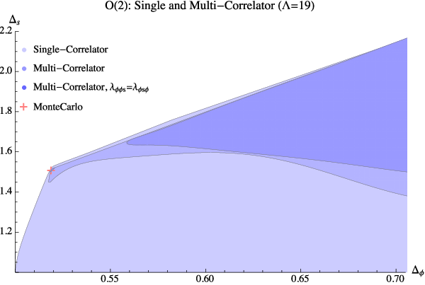
Adding the constraints of crossing symmetry and unitarity for the full system of correlators does not change these bounds without additional assumptions. However, having access to the correlator lets us input information special to the model that does have an effect. We expect that is the only relevant vector in the theory. One way to understand this fact is via the equation of motion at the Wilson-Fisher fixed point in dimensions,
| (3.1) |
This equation implies that the operator is a descendent, so there is a gap in the spectrum of -vector primaries between and the next operator in this sector, which is a linear combination of and . The equation of motion makes sense in perturbation theory . However, it is reasonable to expect gaps in the spectrum to be robust as gets larger. In particular, we expect this gap to persist as . Thus, a gap in the -vector sector reflects the equations of motion of the model.
We do not know if there is sharp experimental evidence for the claim that the model contains exactly one relevant -vector scalar. The cleanest experimental realization of the model is the superfluid transition in 4He [55]. This theory has microscopic symmetry, so one cannot easily determine the number of relevant -vector scalars by counting order parameters. The number could be determined by counting order parameters in systems where the symmetry is emergent.
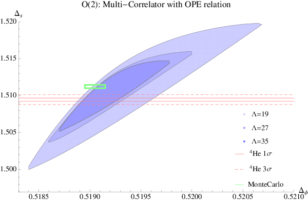
As explained above, it is natural to impose a gap in both the vector and singlet sectors in our formalism, giving rise to the medium blue region in figure 2. Another important constraint is symmetry of the OPE coefficient . Adding this constraint gives the dark blue region in figure 2; a close-up view of the model point is shown in figure 3, which we show for increasing numbers of derivatives (see appendix A). We now have a closed island around the expected position of the model, very close to the original kink in figure 2. The bounds strengthen as increases. However, the allowed regions apparently do not shrink as quickly as in the case of the 3d Ising CFT [52]. Thus, our determination of is unfortunately not competitive with the best available Monte Carlo [56] and experimental [55] results (though it is consistent with both).66 6 Note that 4He experiments cannot easily determine because the symmetry is realized microscopically. Some results constraining have been reported from NMR experiments (e.g., as summarized in [53]) but they are not very precise. We conjecture that including additional crossing relations (such as those involving the symmetric tensor ) will give even stronger bounds; we plan to explore this possibility in future work.
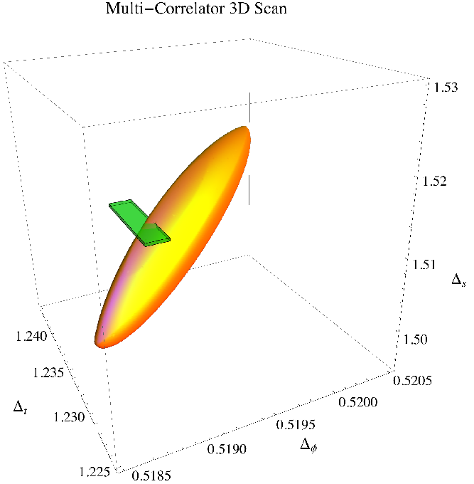
In addition to gaps in the -vector and singlet sectors, we also expect that the model has a single relevant traceless symmetric tensor . Let us finally impose this condition by demanding that has dimension above and scanning over along with . The result is a three-dimensional island for the relevant scalar operator dimensions, which we show in figure 4. Our errors for the symmetric-tensor dimension are much more competitive with previous determinations. By scanning over different values of in the allowed region and computing the allowed range of at , we estimate
| (3.2) |
which is consistent with previous results from the pseudo- expansion approach [57] giving .
3.2 ,

The bounds for are similar to the case of . In figure 5, we show the allowed region of for theories with symmetry, assuming and are the only relevant scalars in their respective representations, and using symmetry of the OPE coefficient . We expect that an additional scan over would yield a 3d island similar to figure 4. By performing this scan at a few values of , we estimate
| (3.3) |
which is consistent with previous results from the pseudo- expansion approach [57] giving .

In figure 6, we show the allowed region of for the model, with the same assumptions as discussed above for . A clear trend is that the allowed region is growing with . For example, at , the allowed region isn’t even an island — it connects to a larger region not shown in the plot. Increasing the number of derivatives to shrinks the region, but it is not as small as in the case of or .
The trend of lower-precision determinations at larger reverses at some point. For example, in figure 1, the allowed region for is smaller again than the region. The relative size of the region and the region is -dependent, and we have not studied the pattern for general in detail. However, as an important check we note that the island in figure 1 is nicely compatible with the expansion (see [15]), giving the point which sits in the upper-left corner of the allowed region.
Finally, we remark that all of the constraints on operator dimensions found above can be reinterpreted in terms of constraints on critical exponents. Following standard critical exponent notation (see [53]), the relations are given by
| (3.4) |
3.3 Current Central Charges
Let be the conserved currents that generate transformations. is an antisymmetric tensor with spin 1 and dimension 2. Its 2-point function is determined by conformal and symmetry to be
| (3.5) |
We call the normalization coefficient from Eq. (3.5) the current central charge.77 7 This name is by analogy with the case of 2d CFTs, where appears as a central element in an affine Kac-Moody algebra. In higher dimensional CFTs, is not an element of a nontrivial algebra in general, though it can be in special cases [37]. The conserved current appears in the sum over antisymmetric-tensor operators in Eq. (2.1). A Ward identity relates the OPE coefficient to . In our conventions
| (3.6) |
where is the free theory value of [60, 61]. In the vector models is known to have the large and expansions [62]
| (3.7) |
Note that both of these expansions predict that will be smaller than the free value.
It is well known that the conformal bootstrap allows one to place upper bounds on OPE coefficients, or equivalently a lower bound on . Previously such bounds were explored in in [6, 10] and in in [22]. To find such a bound, we search for a functional with the following properties (cf. eq. (2.2)):
Notice that compared to (2.2), we have dropped the assumption of the functional being positive on the identity operator contribution and we chose a convenient normalization for . It follows then from the crossing equation (2.1) that
Therefore, finding a functional sets a lower bound on . To improve the bound, we should minimize the RHS of (3.3). We thus seek to minimize
subject to the constraints (3.3). This type of problem can be efficiently solved using SDPB. In this way, we set a lower bound on for all allowed values of , .
We can also set an upper bound on , provided we additionally assume a gap in the spin-1 antisymmetric tensor sector. At this point it is not clear what gap we should assume, but to stay in the spirit of our previous assumptions, we will assume that the dimension of the second spin-1 antisymmetric tensor satisfies , so that the current is the only relevant operator in this sector. We now search for a functional (different from the one above) that satisfies
| (3.28) | |||||
| (3.29) |
and is normalized so that
| (3.30) |
The constraints on coming from the singlet and traceless symmetric-tensor sectors stay the same as in (3.3). An upper bound on then follows from (2.1):
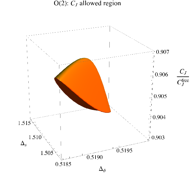
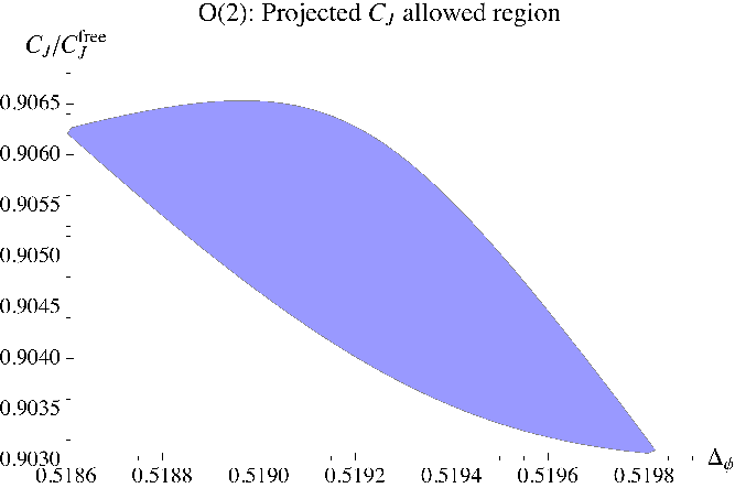
Our upper and lower bounds on , expressed as a function of and , are shown in figures 7 and 8 for and symmetry, respectively. The allowed region for a given consists of a 3d island in space. This determines the current central charge to within the height of the island. For the two physically most interesting cases, and , we find:
| (3.35) |
As an additional check, we also computed for :
| (3.36) |
This result agrees within accuracy with the leading expansion result, [62].
 |
 |
 |
 |
Recently, the current central charge attracted some interest in studies of transport properties of symmetric systems near a quantum critical point, where can be related to the conductivity at zero temperature. In particular, using the OPE it was found in [54] that the asymptotic behavior of conductivity at low temperature is given by
| (3.37) |
where is the conductance quantum. Here, is the (unitless) conductivity at high frequency and zero temperature which is related to as
| (3.38) |
Furthermore, is the central charge of the theory, is the OPE coefficient, and is one of the OPE coefficients, where is the energy-momentum tensor. and are the finite temperature one-point function coefficients:
| (3.39) |
Of all the CFT data that goes into (3.37), we have determined and for the vector models in this work, while was estimated using bootstrap methods before in [15]. The OPE coefficients and can not be determined in our setup, but could in principle be obtained by including the conserved current as an external operator in the crossing equations. The one-point functions and are in principle determined by the spectrum and OPE coefficients of the theory [63]. However, to compute them we would need to know the high-dimension operator spectrum. This is still out of the reach of the conformal bootstrap approach.
Of particular interest for physical applications is the case, which describes superfluid-insulator transitions in systems with two spatial dimensions [64, 65]. Some examples of such systems are thin films of superconducting materials, Josephson junction arrays, and cold atoms trapped in an optical lattice. In these systems the parameter is the high-frequency limit of the conductivity. This quantity has not yet been measured in experiments, but was recently computed in Quantum Monte Carlo simulations [66, 54], [67], and [68] to be , and , respectively88 8 These uncertainties reflect statistical errors but may not include systematic effects, conservatively estimated in [66] to be . We thank Subir Sachdev, Erik Sørensen, and William Witczak-Krempa for correspondence on this point.. Our rigorous result is in excellent agreement with these determinations and is significantly more precise after systematic uncertainties are taken into account.
4 Conclusions
In this work, we used the conformal bootstrap with multiple correlators to set more stringent bounds on the operator spectrum of 3d CFTs with symmetry. The multiple correlator approach works in this setting similarly to the case of -symmetric CFTs – including mixed correlators opens access to parts of the spectrum that are inaccessible with a single correlator. In this work we considered mixed correlators of an singlet and an vector, gaining access to the sector of vectors. We can then additionally input assumptions about the operator spectrum in that sector. As a result, we exclude large portions of the allowed space of CFTs. This reaffirms conclusions from previous works on the 3d Ising model: it is important and fruitful to consider multiple crossing equations. We believe that including mixed correlators will be rewarding in many other bootstrap studies that are currently ongoing.
Specifically, for symmetric CFTs, we found that the scaling dimensions of the lowest vector scalar and singlet scalar are constrained to lie in a closed region in the plane. Our assumptions, besides conformal and symmetry, were crossing symmetry, unitarity, and — crucially — the absence of other relevant scalars in the singlet and vector sectors. This is completely analogous to the -symmetric case where similar assumptions isolate a small allowed region around the Ising model in the plane. Our allowed regions represent rigorous upper and lower bounds on dimensions in the models. In principle, this approach could be used to compute the scaling dimensions of the models to a very high precision, assuming that the allowed region will shrink to a point with increased computational power. However, our results suggest that the region either does not shrink to a point, or the convergence is slow in the present setup. Therefore, our uncertainties are currently larger than the error bars obtained using other methods.99 9 If one is willing to assume that the models live near kinks in our allowed regions, then more precise determinations are possible. In particular, we have not yet resolved the discrepancy between Monte Carlo simulations and experiment for the value of in the model.
Including more correlators could result in significantly improved bounds on operator dimensions. In the case of symmetric CFTs, it would be natural to include the lowest dimension symmetric tensor as an external operator in the crossing equations. In the models, this operator actually has a lower dimension than . This is an important difference from the Ising model, where and are the two lowest dimensional scalars in any sector of the theory. Our present bounds on the lowest symmetric tensor treated it as an internal operator in the crossing equations. Including it as an external operator would open access to many other representations. Perhaps the models are not uniquely determined by the condition of only one relevant singlet and vector scalar, and we must also specify something about these other representations. Studying the models in other dimensions (such as in 5d [22, 28, 30, 69, 70]) may also help to shed light on these issues. We plan to further explore these questions in the future.
In addition to scaling dimensions, it is also important to determine OPE coefficients. Here we presented an example in the computation of the current central charge . In the case of symmetry, this yields the current most precise prediction for the high-frequency conductivity in -symmetric systems at criticality. It will be interesting to extend these mixed-correlator computations to other OPE coefficients in the models such as the stress-tensor central charge and 3-point coefficients appearing in and which control frequency-dependent corrections to conductivity. Pursuing the latter will require implementing the bootstrap for current 4-point functions, a technical challenge for which efforts are ongoing in the bootstrap community.
More generally, the results of this work make it seem likely that scaling dimensions in many other strongly-interacting CFTs can be rigorously determined using the multiple correlator bootstrap. It will be interesting to study mixed correlators in 3d CFTs with fermions and gauge fields – it is plausible that similar islands can be found for the 3d Gross-Neveu models and 3d Chern-Simons and gauge theories coupled to matter. In 4d, we hope that by pursuing the mixed correlator bootstrap we will eventually be able to isolate and rigorously determine the conformal window of QCD. It also be interesting to apply this approach to theories with conformal manifolds to see the emergence of lines and surfaces of allowed dimensions; a concrete application would be to extend the analysis of [14, 23] to mixed correlators and pursue a rigorous study of the dimension of the Konishi operator in supersymmetric Yang-Mills theory at finite . The time is ripe to set sail away from our archipelago and explore the vast ocean of CFTs!
Acknowledgements
We thank Chris Beem, Sheer El-Showk, Luca Iliesiu, Emanuel Katz, Igor Klebanov, Daliang Li, Miguel Paulos, Silviu Pufu, Leonardo Rastelli, Slava Rychkov, Subir Sachdev, Erik Sørensen, Andreas Stergiou, Balt van Rees, William Witczak-Krempa, and Ran Yacoby for discussions. We additionally thank the organizers of the PCTS workshop “Higher Spin Symmetries and Conformal Bootstrap” for facilitating discussions related to this work. The work of DSD is supported by DOE grant number DE-SC0009988 and a William D. Loughlin Membership at the Institute for Advanced Study. The work of DP and FK is supported by NSF grant 1350180. The computations in this paper were run on the Bulldog computing clusters supported by the facilities and staff of the Yale University Faculty of Arts and Sciences High Performance Computing Center, on the Hyperion computing cluster supported by the School of Natural Sciences Computing Staff at the Institute for Advanced Study and on the CERN cluster.
Appendix A Implementation Details
As described in [51], the problem of finding satisfying (2.2) can be transformed into a semidefinite program. Firstly, we must approximate derivatives of , and as positive functions times polynomials in . We do this by computing rational approximations for conformal blocks using the recursion relation described in [51]. Keeping only the polynomial numerator in these rational approximations, (2.2) becomes a “polynomial matrix program” (PMP), which can be solved with SDPB [52].
Three choices must be made to compute the PMP. Firstly, (defined in appendix A of [52]) determines how many poles to include in the rational approximation for conformal blocks. Secondly, determines which derivatives of conformal blocks to include in the functionals . Specifically, we take
| (A.1) |
Some of these derivatives vanish by symmetry properties of . The total number of nonzero components of is
| (A.2) |
Finally, we must choose which spins to include in the PMP. The number of spins depends on as follows
| (A.3) |
We use Mathematica to compute and store tables of derivatives of conformal blocks. Another Mathematica program reads these tables, computes the polynomial matrices corresponding to the ’s, and uses the package SDPB.m to write the associated PMP to an xml file. This xml file is then used as input to SDPB. Our settings for SDPB are given in table 1.
| 19 | 27 | 35 | 39 | |
| 14 | 20 | 30 | 36 | |
| spins | ||||
| precision | 448 | 576 | 768 | 896 |
| findPrimalFeasible | True | True | True | True |
| findDualFeasible | True | True | True | True |
| detectPrimalFeasibleJump | True | True | True | True |
| detectDualFeasibleJump | True | True | True | True |
| dualityGapThreshold | ||||
| primalErrorThreshold | ||||
| dualErrorThreshold | ||||
| initialMatrixScalePrimal | ||||
| initialMatrixScaleDual | ||||
| feasibleCenteringParameter | 0.1 | 0.1 | 0.1 | 0.1 |
| infeasibleCenteringParameter | 0.3 | 0.3 | 0.3 | 0.3 |
| stepLengthReduction | 0.7 | 0.7 | 0.7 | 0.7 |
| choleskyStabilizeThreshold | ||||
| maxComplementarity |
Finally let us conclude with some comments on the precision of the plots presented in the main text. Conformal blocks of correlation functions involving operators of nonequal dimensions depend nontrivially on the difference of the dimensions. Hence, when computing the boundary of various allowed regions, it is convenient to perform a scan over a lattice of points. The vectors generating the lattice points are shown in table 2. The smooth regions shown in figs. 1, 3, 5, and 6 are the results of a least-squares fit, subject to the constraint that allowed lattice points should lie inside the curves while excluded ones lie outside. In table 2 we also show the maximal perpendicular distance of these points to the curves.
The bounds on shown in figures 7 and 8 were computed for the lattices of points that were found to be allowed in figures 3 and 5. For each point on the lattice, the bound on was determined to a precision of . The smooth regions were obtained by interpolation and the maximum distance of the computed points to the boundry of the shaded region is again reported in table 2.
| allowed | excluded | ||||
| 0.00025 | 0.00060 | ||||
| 0.000084 | 0.00025 | ||||
| 0.00021 | 0.00062 | ||||
| 0.00043 | 0.0020 | ||||
| 0.00044 | 0.0019 | ||||
| 0.00041 | 0.0013 | ||||
| 0.00040 | 0.00041 | ||||
| 0.00048 | 0.00048 | ||||
| 0.00029 | 0.00062 | ||||
| 0.00014 | 0.00023 | ||||
| : | 0.00005 | - | |||
| : | 0.0001 | - |
Appendix B Symmetric Tensor Scan
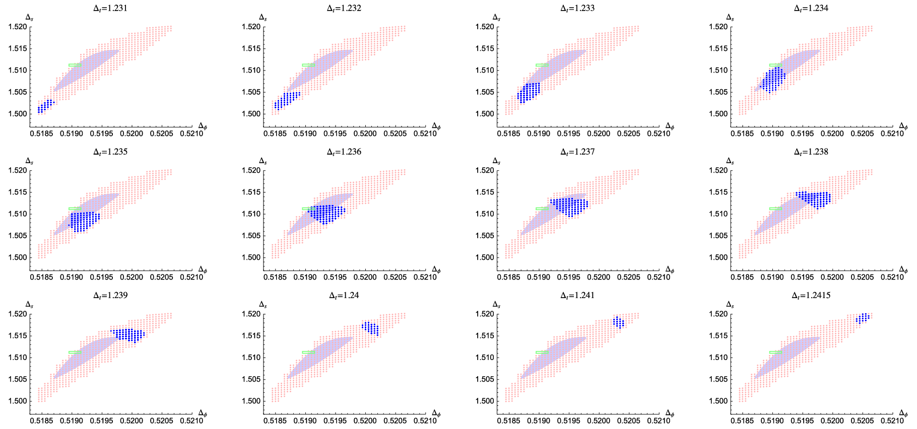
In this appendix we collect some detailed scans of the allowed region of space for models with . The results for the model are also presented as a 3d plot in figure 4. Here we show plots in the plane at fixed values of . The scans for , and are shown in figs. 9, 10, and 11, respectively. Blue points represent the allowed region at . The light blue shaded area is the allowed region at , but without any assumptions in symmetric tensor sector; those are the same allowed regions shown in figs. 3, 5, and 6. The final allowed regions with the assumptions on are thus given by the intersections of the dark blue and light blue regions.
Qualitatively the picture is the same for each value of and we expect that the projections of the 3d plot into the plane will look similar for even higher values of . In particular, the lowest allowed values of are obtained at the lower left corner of the allowed region in the plane, while the greatest values are obtained at upper right corner of the allowed region. This allows us to find general bounds on without doing a whole scan over the plane; it is enough to find bounds on at the corner points.


References
- [1] S. Ferrara, A. F. Grillo, and R. Gatto, “Tensor representations of conformal algebra and conformally covariant operator product expansion,” Annals Phys. 76 (1973) 161–188.
- [2] A. M. Polyakov, “Nonhamiltonian approach to conformal quantum field theory,” Zh. Eksp. Teor. Fiz. 66 (1974) 23–42.
- [3] R. Rattazzi, V. S. Rychkov, E. Tonni, and A. Vichi, “Bounding scalar operator dimensions in 4D CFT,” JHEP 12 (2008) 031, arXiv:0807.0004 [hep-th].
- [4] V. S. Rychkov and A. Vichi, “Universal Constraints on Conformal Operator Dimensions,” Phys. Rev. D80 (2009) 045006, arXiv:0905.2211 [hep-th].
- [5] F. Caracciolo and V. S. Rychkov, “Rigorous Limits on the Interaction Strength in Quantum Field Theory,” Phys. Rev. D81 (2010) 085037, arXiv:0912.2726 [hep-th].
- [6] D. Poland and D. Simmons-Duffin, “Bounds on 4D Conformal and Superconformal Field Theories,” JHEP 1105 (2011) 017, arXiv:1009.2087 [hep-th].
- [7] R. Rattazzi, S. Rychkov, and A. Vichi, “Central Charge Bounds in 4D Conformal Field Theory,” Phys. Rev. D83 (2011) 046011, arXiv:1009.2725 [hep-th].
- [8] R. Rattazzi, S. Rychkov, and A. Vichi, “Bounds in 4D Conformal Field Theories with Global Symmetry,” J. Phys. A44 (2011) 035402, arXiv:1009.5985 [hep-th].
- [9] A. Vichi, “Improved bounds for CFT’s with global symmetries,” JHEP 1201 (2012) 162, arXiv:1106.4037 [hep-th].
- [10] D. Poland, D. Simmons-Duffin, and A. Vichi, “Carving Out the Space of 4D CFTs,” JHEP 1205 (2012) 110, arXiv:1109.5176 [hep-th].
- [11] S. Rychkov, “Conformal Bootstrap in Three Dimensions?,” arXiv:1111.2115 [hep-th].
- [12] S. El-Showk, M. F. Paulos, D. Poland, S. Rychkov, D. Simmons-Duffin, and A. Vichi, “Solving the 3D Ising Model with the Conformal Bootstrap,” Phys.Rev. D86 (2012) 025022, arXiv:1203.6064 [hep-th].
- [13] P. Liendo, L. Rastelli, and B. C. van Rees, “The Bootstrap Program for Boundary CFTd,” JHEP 1307 (2013) 113, arXiv:1210.4258 [hep-th].
- [14] C. Beem, L. Rastelli, and B. C. van Rees, “The Superconformal Bootstrap,” Phys.Rev.Lett. 111 (2013) 071601, arXiv:1304.1803 [hep-th].
- [15] F. Kos, D. Poland, and D. Simmons-Duffin, “Bootstrapping the vector models,” JHEP 1406 (2014) 091, arXiv:1307.6856 [hep-th].
- [16] S. El-Showk, M. Paulos, D. Poland, S. Rychkov, D. Simmons-Duffin, and A. Vichi, “Conformal field theories in fractional dimensions,” Phys. Rev. Lett. 112 (Apr, 2014) 141601, arXiv:1309.5089 [hep-th].
- [17] L. F. Alday and A. Bissi, “The superconformal bootstrap for structure constants,” JHEP 1409 (2014) 144, arXiv:1310.3757 [hep-th].
- [18] D. Gaiotto, D. Mazac, and M. F. Paulos, “Bootstrapping the 3d Ising twist defect,” JHEP 1403 (2014) 100, arXiv:1310.5078 [hep-th].
- [19] D. Bashkirov, “Bootstrapping the SCFT in three dimensions,” arXiv:1310.8255 [hep-th].
- [20] M. Berkooz, R. Yacoby, and A. Zait, “Bounds on superconformal theories with global symmetries,” JHEP 1408 (2014) 008, arXiv:1402.6068 [hep-th].
- [21] Y. Nakayama and T. Ohtsuki, “Approaching the conformal window of symmetric Landau-Ginzburg models using the conformal bootstrap,” Phys.Rev. D89 no. 12, (2014) 126009, arXiv:1404.0489 [hep-th].
- [22] Y. Nakayama and T. Ohtsuki, “Five dimensional -symmetric CFTs from conformal bootstrap,” Phys.Lett. B734 (2014) 193–197, arXiv:1404.5201 [hep-th].
- [23] L. F. Alday and A. Bissi, “Generalized bootstrap equations for SCFT,” JHEP 1502 (2015) 101, arXiv:1404.5864 [hep-th].
- [24] S. M. Chester, J. Lee, S. S. Pufu, and R. Yacoby, “The superconformal bootstrap in three dimensions,” JHEP 1409 (2014) 143, arXiv:1406.4814 [hep-th].
- [25] F. Caracciolo, A. C. Echeverri, B. von Harling, and M. Serone, “Bounds on OPE Coefficients in 4D Conformal Field Theories,” JHEP 1410 (2014) 20, arXiv:1406.7845 [hep-th].
- [26] Y. Nakayama and T. Ohtsuki, “Bootstrapping phase transitions in QCD and frustrated spin systems,” Phys.Rev. D91 no. 2, (2015) 021901, arXiv:1407.6195 [hep-th].
- [27] M. F. Paulos, “JuliBootS: a hands-on guide to the conformal bootstrap,” arXiv:1412.4127 [hep-th].
- [28] J.-B. Bae and S.-J. Rey, “Conformal Bootstrap Approach to O(N) Fixed Points in Five Dimensions,” arXiv:1412.6549 [hep-th].
- [29] C. Beem, M. Lemos, P. Liendo, L. Rastelli, and B. C. van Rees, “The superconformal bootstrap,” arXiv:1412.7541 [hep-th].
- [30] S. M. Chester, S. S. Pufu, and R. Yacoby, “Bootstrapping O(N) Vector Models in ,” arXiv:1412.7746 [hep-th].
- [31] N. Bobev, S. El-Showk, D. Mazac, and M. F. Paulos, “Bootstrapping the Three-Dimensional Supersymmetric Ising Model,” arXiv:1502.04124 [hep-th].
- [32] N. Bobev, S. El-Showk, D. Mazac, and M. F. Paulos, “Bootstrapping SCFTs with Four Supercharges,” arXiv:1503.02081 [hep-th].
- [33] I. Heemskerk, J. Penedones, J. Polchinski, and J. Sully, “Holography from Conformal Field Theory,” JHEP 0910 (2009) 079, arXiv:0907.0151 [hep-th].
- [34] I. Heemskerk and J. Sully, “More Holography from Conformal Field Theory,” JHEP 1009 (2010) 099, arXiv:1006.0976 [hep-th].
- [35] A. L. Fitzpatrick, J. Kaplan, D. Poland, and D. Simmons-Duffin, “The Analytic Bootstrap and AdS Superhorizon Locality,” JHEP 1312 (2013) 004, arXiv:1212.3616 [hep-th].
- [36] Z. Komargodski and A. Zhiboedov, “Convexity and Liberation at Large Spin,” JHEP 1311 (2013) 140, arXiv:1212.4103 [hep-th].
- [37] C. Beem, M. Lemos, P. Liendo, W. Peelaers, L. Rastelli, et al., “Infinite Chiral Symmetry in Four Dimensions,” Commun.Math.Phys. 336 no. 3, (2015) 1359–1433, arXiv:1312.5344 [hep-th].
- [38] A. L. Fitzpatrick, J. Kaplan, and M. T. Walters, “Universality of Long-Distance AdS Physics from the CFT Bootstrap,” JHEP 1408 (2014) 145, arXiv:1403.6829 [hep-th].
- [39] C. Beem, L. Rastelli, and B. C. van Rees, “W Symmetry in six dimensions,” arXiv:1404.1079 [hep-th].
- [40] L. F. Alday, A. Bissi, and T. Lukowski, “Lessons from crossing symmetry at large N,” arXiv:1410.4717 [hep-th].
- [41] S. M. Chester, J. Lee, S. S. Pufu, and R. Yacoby, “Exact Correlators of BPS Operators from the 3d Superconformal Bootstrap,” JHEP 1503 (2015) 130, arXiv:1412.0334 [hep-th].
- [42] A. Kaviraj, K. Sen, and A. Sinha, “Analytic bootstrap at large spin,” arXiv:1502.01437 [hep-th].
- [43] L. F. Alday, A. Bissi, and T. Lukowski, “Large spin systematics in CFT,” arXiv:1502.07707 [hep-th].
- [44] A. Kaviraj, K. Sen, and A. Sinha, “Universal anomalous dimensions at large spin and large twist,” arXiv:1504.00772 [hep-th].
- [45] A. L. Fitzpatrick, J. Kaplan, M. T. Walters, and J. Wang, “Eikonalization of Conformal Blocks,” arXiv:1504.01737 [hep-th].
- [46] S. El-Showk and M. F. Paulos, “Bootstrapping Conformal Field Theories with the Extremal Functional Method,” Phys.Rev.Lett. 111 no. 24, (2013) 241601, arXiv:1211.2810 [hep-th].
- [47] F. Gliozzi, “More constraining conformal bootstrap,” Phys.Rev.Lett. 111 (2013) 161602, arXiv:1307.3111.
- [48] F. Gliozzi and A. Rago, “Critical exponents of the 3d Ising and related models from Conformal Bootstrap,” JHEP 1410 (2014) 42, arXiv:1403.6003 [hep-th].
- [49] F. Gliozzi, P. Liendo, M. Meineri, and A. Rago, “Boundary and Interface CFTs from the Conformal Bootstrap,” arXiv:1502.07217 [hep-th].
- [50] S. El-Showk, M. F. Paulos, D. Poland, S. Rychkov, D. Simmons-Duffin, et al., “Solving the 3d Ising Model with the Conformal Bootstrap II. c-Minimization and Precise Critical Exponents,” J.Stat.Phys. 157 (2014) 869, arXiv:1403.4545 [hep-th].
- [51] F. Kos, D. Poland, and D. Simmons-Duffin, “Bootstrapping Mixed Correlators in the 3D Ising Model,” JHEP 1411 (2014) 109, arXiv:1406.4858 [hep-th].
- [52] D. Simmons-Duffin, “A Semidefinite Program Solver for the Conformal Bootstrap,” arXiv:1502.02033 [hep-th].
- [53] A. Pelissetto and E. Vicari, “Critical phenomena and renormalization-group theory,” Phys. Rept. 368 (2002) 549–727, arXiv:cond-mat/0012164.
- [54] E. Katz, S. Sachdev, E. S. Sørensen, and W. Witczak-Krempa, “Conformal field theories at nonzero temperature: Operator product expansions, Monte Carlo, and holography,” Phys.Rev. B90 no. 24, (2014) 245109, arXiv:1409.3841 [cond-mat.str-el].
- [55] J. Lipa, J. Nissen, D. Stricker, D. Swanson, and T. Chui, “Specific heat of liquid helium in zero gravity very near the lambda point,” Phys.Rev. B68 (2003) 174518.
- [56] M. Campostrini, M. Hasenbusch, A. Pelissetto, and E. Vicari, “The Critical exponents of the superfluid transition in He-4,” Phys.Rev. B74 (2006) 144506, arXiv:cond-mat/0605083 [cond-mat].
- [57] P. Calabrese and P. Parruccini, “Harmonic crossover exponents in O(n) models with the pseudo-epsilon expansion approach,” Phys.Rev. B71 (2005) 064416, arXiv:cond-mat/0411027 [cond-mat].
- [58] M. Campostrini, M. Hasenbusch, A. Pelissetto, P. Rossi, and E. Vicari, “Critical exponents and equation of state of the three-dimensional Heisenberg universality class,” Phys.Rev. B65 (2002) 144520, arXiv:cond-mat/0110336 [cond-mat].
- [59] M. Hasenbusch, “Eliminating leading corrections to scaling in the three-dimensional O(N) symmetric phi**4 model: N=3 and N=4,” J.Phys. A34 (2001) 8221–8236, arXiv:cond-mat/0010463 [cond-mat].
- [60] H. Osborn and A. Petkou, “Implications of conformal invariance in field theories for general dimensions,” Annals Phys. 231 (1994) 311–362, arXiv:hep-th/9307010 [hep-th].
- [61] A. Petkou, “Conserved currents, consistency relations and operator product expansions in the conformally invariant O(N) vector model,” Annals Phys. 249 (1996) 180–221, arXiv:hep-th/9410093 [hep-th].
- [62] A. C. Petkou, “C(T) and C(J) up to next-to-leading order in 1/N in the conformally invariant O(N) vector model for ,” Phys.Lett. B359 (1995) 101–107, arXiv:hep-th/9506116 [hep-th].
- [63] S. El-Showk and K. Papadodimas, “Emergent Spacetime and Holographic CFTs,” JHEP 1210 (2012) 106, arXiv:1101.4163 [hep-th].
- [64] M.-C. Cha, M. P. A. Fisher, S. M. Girvin, M. Wallin, and A. P. Young, “Universal conductivity of two-dimensional films at the superconductor-insulator transition,” Phys. Rev. B 44 (Oct, 1991) 6883–6902. http://link.aps.org/doi/10.1103/PhysRevB.44.6883.
- [65] J. Šmakov and E. Sørensen, “Universal scaling of the conductivity at the superfluid-insulator phase transition,” Phys. Rev. Lett. 95 (Oct, 2005) 180603. http://link.aps.org/doi/10.1103/PhysRevLett.95.180603.
- [66] W. Witczak-Krempa, E. Sørensen, and S. Sachdev, “The dynamics of quantum criticality via Quantum Monte Carlo and holography,” Nature Phys. 10 (2014) 361, arXiv:1309.2941 [cond-mat.str-el].
- [67] K. Chen, L. Liu, Y. Deng, L. Pollet, and N. Prokof’ev, “Universal conductivity in a two-dimensional superfluid-to-insulator quantum critical system,” Phys. Rev. Lett. 112 (Jan, 2014) 030402. http://link.aps.org/doi/10.1103/PhysRevLett.112.030402.
- [68] S. Gazit, D. Podolsky, and A. Auerbach, “Critical capacitance and charge-vortex duality near the superfluid-to-insulator transition,” Phys. Rev. Lett. 113 (Dec, 2014) 240601. http://link.aps.org/doi/10.1103/PhysRevLett.113.240601.
- [69] L. Fei, S. Giombi, and I. R. Klebanov, “Critical models in dimensions,” Phys.Rev. D90 no. 2, (2014) 025018, arXiv:1404.1094 [hep-th].
- [70] L. Fei, S. Giombi, I. R. Klebanov, and G. Tarnopolsky, “Three loop analysis of the critical O(N) models in dimensions,” Phys.Rev. D91 no. 4, (2015) 045011, arXiv:1411.1099 [hep-th].