Electronic structure and core-level spectra of light actinide dioxides in the dynamical mean-field theory
Abstract
The local-density approximation combined with the dynamical mean-field theory (LDA+DMFT) is applied to the paramagnetic phase of light actinide dioxides: UO2, NpO2, and PuO2. The calculated band gaps and the valence-band electronic structure are in a very good agreement with the optical absorption experiments as well as with the photoemission spectra. The hybridization of the actinide 5f shell with the 2p states of oxygen is found to be relatively large, it increases the filling of the 5f orbitals from the nominal ionic configurations with two, three, and four electrons to nearly half-integer values 2.5, 3.4 and 4.4. The large hybridization leaves an imprint also on the core-level photoemission spectra in the form of satellite peaks. It is demonstrated that these satellites are accurately reproduced by the LDA+DMFT calculations.
pacs
71.20.Gj, 79.60.i, 71.15.m, 71.27.+aI Introduction
Actinide dioxides are correlations-driven insulators [1, 2] that display a variety of complex ordered phases at low temperatures.[3] They crystallize in the CaF2 structure (space group Fmm), with eight-coordinated actinide atoms, and four-coordinated oxygen atoms. Due to the interplay of electron correlations, spin-orbital coupling and crystal field effects, the theoretical modeling of the electronic structure of these oxides presents numerous challenges.
The conventional Kohn–Sham density-functional theory (DFT) in the local-density (LDA) and generalized gradient approximations fails to explain the insulating character of the oxides.[4] The band-gap problem was addressed a number of times using orbital-dependent functionals such as the self-interaction corrected LDA,[5] LDA+U,[6] or the hybrid exchange-correlation functionals.[7, 8, 4] All of these calculations lead to insulators but the opening of the gap is intimately linked with the appearance of a long-range magnetic order. That is not satisfactory since the oxides retain the gap also in the high-temperature paramagnetic phase. Moreover, the orbital-dependent functionals predict a large magnetic moment at the plutonium atoms in PuO2 in disagreement with experiments.[9] These issues appear to be a rather general shortcoming of static mean-field approximations that build on a single determinant of Kohn–Sham orbitals.
The dynamical mean-field theory (DMFT) is able to describe correlated nonmagnetic insulators.[10] This method, in combination with the density-functional theory, was successfully applied to selected actinide dioxides recently,[11, 12] and it indeed yields an insulating electronic structure without any long-range order and without any local magnetic moments in PuO2. In the present paper, we follow up on our previous study of the plutonium dioxide,[12] where we employed a crystal-field potential deduced from experiments and assumed a simplified spherically symmetric hybridization of the plutonium 5f shell with the surrounding electronic states. Here we relax these simplifications and determine the quantities entirely from first principles. We investigate also the paramagnetic phases of UO2 and NpO2 in order to visualize trends in the behavior of the computed properties when the filling of the actinide 5f shell changes.
II Methods
II.1 LDA
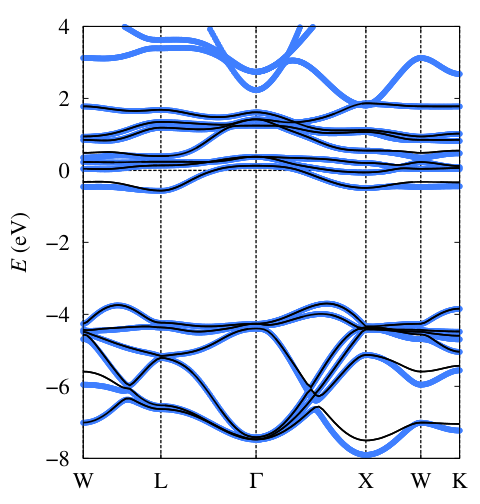
We start with all-electron LDA calculations[13] of the band structure of the dioxides at the experimental lattice constants (Tab. 1). We take into account scalar-relativistic effects as well as the spin-orbital coupling. To this end, we employ the wien2k package[14] with the following parameters: the radii of the muffin-tin spheres are for actinide atoms and for oxygen atoms, the basis-set cutoff is defined with , and the Brillouin zone is sampled with 3375 k points (120 k points in the irreducible wedge). The computed electronic structure is essentially identical to the nonmagnetic LDA results shown in Ref. 6.
The LDA bands of the actinide 5f and oxygen 2p origin are subsequently mapped onto a tight-binding model with the aid of the wannier90 code[15] in conjunction with the wien2wannier interface.[16] This effective model then serves as a base for the LDA+DMFT calculations. The tight-binding representation is not perfect, there are some deviations from the original band structure that originate mainly in the neglected overlap of the actinide 6d states with the oxygen 2p orbitals. The largest differences appear in UO2, they are explicitly illustrated in Fig. 1. It is possible to get a closer match even for UO2, but the resulting 5f Wannier functions have a varied spatial extension which complicates their interpretation as an atomic f shell later on.
II.2 LDA+DMFT
The dynamical mean-field modeling of correlations among the 5f electrons amounts to adding a local selfenergy to the 5f shell of each actinide atom in the tight-binding model . The selfenergy is taken from an auxiliary impurity model that consists of one fully interacting f shell (the impurity) embedded in a self-consistent non-interacting medium .[10]
The auxiliary model without the f–f interactions can be written as
| (1) |
where the lower-case indices label the f orbitals and run from 1 to 14 (or they can be understood as combinations of the magnetic quantum number and the spin projection ), and the upper-case indices label the orbitals of the effective medium that is usually referred to as bath. We truncate the bath to contain only 14 orbitals so that the local hamiltonian , the bath hamiltonian as well as the hybridization are all matrices. The actual determination of , and is discussed in detail in appendix A. Here we just note that they cannot be reduced to a diagonal form due to non-commutativity of the cubic hybridization with the spin-orbital coupling.
The truncation of the bath is necessary because the Lanczos method, which we employ to solve the impurity model, cannot handle much larger systems. In insulating oxides, the small bath is well justified on the physical grounds: the environment of the 5f shell is dominated by the oxygen ligands and hence a small impurity model analogous to the ligand-field model should accurately represent the dynamics of the 5f shell and its surroundings. High accuracy of these small models was demonstrated many times in the context of core-level spectroscopies,[17] recently for instance in Ref. 18, as well as in applications to the valence-band electronic structure of transition-metal oxides.[19]
The complete interacting impurity model is defined as where is the Coulomb repulsion among the f orbitals,
| (2) |
The matrix elements are decomposed into the radial expectation values – the Slater integrals , and the angular expectation values – the Gaunt coefficients. The latter are fully determined by the assumption that the angular parts of the local orbitals are spherical harmonics. The Slater integrals are assumed identical for all three oxides. They are set to eV, eV, eV and eV. The average Coulomb repulsion has a value close to Ref. 11 to facilitate comparison with this earlier study. The remaining Slater integrals are chosen to obtain the average exchange eV while keeping the ratios and equal to their Hartree–Fock values.[20]
The second term in Eq. (2) is the double-counting correction that removes the Hartree-like contribution already included in the LDA band structure . In the paramagnetic phase, the correction can be simplified to an isotropic form, . We approximate by the so-called fully localized limit , where is the self-consistently determined number of 5f electrons.[21, 22] The isotropic form of the double counting is still only approximate even in the paramagnetic state. It is accurate enough for getting the correct position of the 5f states with respect to the ligand bands, but it is possibly insufficient when it comes to crystal-field effects that occur at a much smaller energy scale, especially in the case of 4f electrons.[23]
The selfenergy in the impurity model is computed using an in-house exact-diagonalization code that combines the implicitly restarted Lanczos method for calculation of the bottom of the many-body spectrum [24] with the band Lanczos method for evaluation of the one-particle Green’s function.[25] The calculations are performed at room temperature ( K), well within the paramagnetic phase. To lessen the computational demands, the Fock space is reduced in a manner analogous to the method developed for Ce compounds by Gunnarsson and Schönhammer.[26] Details of the impurity solver are discussed in appendix B.
II.3 Photoemission spectra
The valence-band photoemission intensity can be evaluated using the Fermi’s golden rule. If the energy and angular dependence of the dipole matrix elements is neglected, the angle-resolved photoelectron spectrum is proportional to the one-particle spectral density of the tight-binding model,11 1 We use the following simplified notation: wherever we add a scalar to an operator or to a matrix, it is to be understood as adding the scalar only to the diagonal elements. That is, and , where and stand for the identity operator and the identity matrix.
| (3) |
A finite imaginary part of the one-particle energy, , was introduced to model the life-time broadening of the valence states together with the experimental resolution. The trace in Eq. (3) runs over all valence states or over a subset of orbitals (actinide 5f or oxygen 2p) if an orbital-resolved signal is desired. The angle-integrated photoelectron spectrum is proportional to the integral of the spectral density over the first Brillouin zone.
Apart from the valence electronic structure, the impurity model of the dynamical mean-field theory provides a means to calculate also the photoemission from core states (x-ray photoemission spectra, XPS)[28, 29, 30] at the level of the so-called multiplet ligand-field theory.[17] To that end, we add a core state and the free-electron states to the impurity model,
| (4) |
where is the energy of the core state, are the energies of the free-electron states, is the number of f electrons, and is the strength of the Coulomb repulsion between the core electrons and the f electrons. The degeneracy of the core state is neglected and hence there is only one core-valence Slater integral.
Employing the Fermi’s golden rule, the probability of the emission of an electron from the core level to a scattering state with an energy can be written as[26, 17]
| (5) |
where is the many-body ground state of the converged DMFT impurity model (that is, the initial state of the photoemission process), is the corresponding ground-state energy, and simulates the life-time broadening of the core state. As in the case of the valence spectra, we neglected the energy dependence of the dipole matrix elements. In addition, we assumed that the free-electron density of states is a constant in the energy window of interest.
The expression shown in Eq. (5) applies at zero temperature, K. The finite-temperature case is analogous to the finite-temperature formula for the one-particle Green’s function, Eqs. (19), discussed in appendix B. Just like the Green’s function, the photoemission intensity is computed using the Lanczos method.
In the course of derivation of Eq. (5), the and degrees of freedom were integrated out and hence the final-state hamiltonian , which enters the denominator of Eq. (5), involves only the f orbitals and the ligand states. Notably, has the same form as , only the diagonal elements of are altered. To make the model more realistic, we scale down the hybridization parameters in the final-state hamiltonian , , . The hybridization between the f shell and the ligand orbitals is reduced due to a contraction of the 5f wave functions when the core hole is present.[31, 17] The reduction of the hybridization parameters can be incorporated into the hamiltonian of Eq. (4) by introducing an extra term
| (6) |
This term does not have any transparent physical interpretation but it can still be used to formally check that the rescaling in the final state is compatible with the steps that led from Eq. (4) to Eq. (5).
III Results and discussion
| (Å) | gap (eV) | ||||
|---|---|---|---|---|---|
| LDA | DMFT | theory | experiment | ||
| UO2 | 5.470 | 2.8 | 2.5 | 1.9 | 2.1 (Ref. 1) |
| NpO2 | 5.432 | 3.8 | 3.4 | 2.5 | 2.8 (Ref. 2) |
| PuO2 | 5.396 | 4.8 | 4.4 | 2.5 | 2.8 (Ref. 2) |
III.1 Valence-band electronic structure

The LDA+DMFT calculations result in an insulating electronic structure for all three investigated dioxides. The obtained band gaps are listed in Tab. 1 together with the corresponding experimental data. The calculations slightly underestimate the gaps, which could be straightforwardly fixed by an increased value of the Coulomb . Nevertheless, we get the correct trend in the magnitude of the gap across the three oxides even without any such fine tuning, simply with the same Coulomb parameters in all cases. This indicates that the material-specific screening of the Coulomb interaction is accurately represented already in the employed minimal model of the valence electronic structure. An analogous conclusion was reached in a recent LDA+DMFT study of transition-metal oxides.[36]
The -integrated spectral density corresponding to the actinide 5f states is shown in Fig. 2 in comparison with the angle-integrated x-ray photoelectron spectra measured with incident photons at the aluminum line (1487 eV). At this energy, the photoionization cross section for the oxygen 2p states is negligible and hence the experimental data contain essentially clean 5f signal. The total spectral density is measured with incident photons at He II line (40.8 eV) as their cross section with actinide 5f and oxygen 2p states is approximately equal. Comparison of He II spectra of PuO2 with our LDA+DMFT calculations is shown in Ref. 37.
Inspecting the case of UO2 in Fig. 2 first, we see three distinct features in the occupied part of the theoretical spectrum: the main 5f bands near eV, a satellite peak near eV, and a broader feature between eV and eV. The last feature coincides with the location of the oxygen 2p bands and reflects the hybridization of the 5f states with the ligands. The three features are discernible also in the spectra of NpO2 and PuO2, only the 2p bands move closer to the main 5f peak, and eventually overlap with this peak in PuO2. The theoretical calculations closely reproduce the shape of the experimental spectra as well as their evolution from UO2 to PuO2, which demonstrates the accuracy of the LDA+DMFT modeling of the electronic structure.
The momentum-resolved spectral density is shown as a color map in Fig. 3. The dispersion of the 5f bands is approximately 0.5 eV in UO2 and it increases only a little to about 0.75 eV in PuO2. The hybrid DFT calculations predict a much larger increase of the 5f bands dispersion in PuO2 due to the degeneracy of the plutonium 5f and oxygen 2p bands (Fig. 2) and a consequent enhancement of the effects of hybridization.[7, 8, 4] Our calculations suggest that such increase of the 5f states dispersion is an artifact of the single-determinant approximation employed in the DFT calculations. Although the angular-resolved photoemission (ARPES) experiments were performed on PuO2, the acquired data are not able to resolve the issue yet due to the lack of orbital resolution (the measurements were done with the He II light source).[38] The analysis of ARPES data is more straightforward in UO2 where the 5f bands are well separated and it is possible to read out their dispersion.[39] It comes out as about 0.13 eV, which is considerably smaller than our result plotted in Fig. 3. A large part of the discrepancy can be attributed to the smearing of the experimental data that merges the two bands into a single peak with an apparent dispersion approximately 50% smaller than the resolved bands. The multiband composition of this single peak shows up in the experiment as a variation of the peak’s shape along the momentum path.
III.2 Screening of the Coulomb interaction
It was demonstrated in the previous section and also in Ref. 11 that the LDA+DMFT method yields an accurate electronic structure if the Coulomb is set around eV, or perhaps even larger since our gaps (Tab. 1) are slightly underestimated. On the other hand, the LDA+U method recovers the correct band gaps in the low-temperature ordered phases already with around 4.0 eV.[6] This difference originates in the different ways the screening by oxygen ligands is accounted for in the two methods. In LDA+DMFT, the oxygen states explicitly enter the impurity solver as the bath and hence the used in the solver does not include the screening by these states. The LDA+U method, on the other hand, is a static limit of the LDA+DMFT where a simplified Hartree–Fock approximation in the atomic limit plays the role of the impurity solver. In this case, the screening by the ligand states can enter the calculations only implicitly in the form of a reduced .
The so-called Hubbard I approximation[40, 41] is analogous to the LDA+U method with respect to the screening of the on-site Coulomb interaction. In the same time, it allows for a description of the paramagnetic phase and hence can be straightforwardly compared to our LDA+DMFT results. The impurity model for the Hubbard I approximation is given by Eq. (1) with and . Figure 4 shows that the spectral density of UO2 from the LDA+Hubbard I method combined with a reduced eV is almost identical to the spectral density from the LDA+DMFT calculations with eV and with all other inputs unchanged. It is the screening by the ligand states that is responsible for the difference in the Coulomb parameter. The same behavior is found also in NpO2 and PuO2 (not shown). A related discussion of the screening effects in transition metal oxides can be found in Ref. 36.
The close similarity between the LDA+Hubbard I and LDA+DMFT spectra of UO2 indicates that the main 5f peak near eV is a lower Hubbard band. It was argued in Ref. 11 that this feature is a Zhang–Rice state resulting from a coupling of the local moment in the 5f shell to a hole in the ligand orbitals.[42] But since the Hubbard I approximation is clearly able to describe this peak, it cannot originate in the Zhang–Rice physics because the Hubbard I selfenergy has no knowledge of the ligand states.
III.3 Core-level spectra
The nominal electronic configuration of the actinide atoms in the investigated dioxides is the ion, which translates to the number of 5f electrons equal two, three, and four in UO2, NpO2, and PuO2, respectively. Our LDA+DMFT calculations converge to solutions with more electrons in the 5f Wannier orbitals, with being close to half-integer values, see Tab. 1. A similarly increased filling of the 5f shell was reported previously in LDA+U, hybrid DFT, and embedded-cluster calculations.[12, 39, 46] The enhancement of the 5f occupation indicates a large covalent mixing (hybridization) between the actinide 5f states and oxygen 2p states. An evidence of such mixing was found also in the experimental core-level spectra where the hybridization with ligands is responsible for the appearance of satellite peaks.[45] An analogous half-integer occupation of the valence f shell is well established in CeO2 on the basis of the core-level spectroscopy.[47, 48, 49] Surprisingly, the earlier LDA+DMFT study of the actinide dioxides reported an integer occupation of the 5f shell in all of them.[11]
In order to test whether our estimates of are compatible with the measured core-level spectra, we have calculated the photoemission from the 4f states using the method outlined in Sec. II.3. Since the theory is formulated for a non-degenerate core state, the total 4f spectrum is approximated as a sum of two independent components (4f5/2 and 4f7/2) that are weighted with the statistical ratio . The splitting between the 4f5/2 and 4f7/2 levels is taken from the all-electron LDA: 11.0 eV (UO2), 11.8 eV (NpO2), and 12.6 eV (PuO2). We employ two empirical parameters in the calculations of the core-level spectra: the core-valence Coulomb repulsion, eV, and the scaling factor of the hybridization in the final state, . We keep these parameters the same for all three oxides. Our results are plotted in Fig. 5 together with the experimental spectra. The satellites are well reproduced which indicates that the LDA+DMFT fillings are indeed reasonable. It is possible to analyze individual contributions to each of the spectral features,[45, 46] but we do not enter that level of detail here.
III.4 Crystal-field states
| ground state | excited levels (meV) | ||||
|---|---|---|---|---|---|
| multiplicity | (multiplicity in brackets) | ||||
| UO2 | theory | 3 | 161 (1) | 164 (3) | 184 (2) |
| Ref. 50 | 150 | 170 | |||
| NpO2 | theory | 4 | 76 (4) | 302 (2) | |
| Ref. 51 | 55 | – | |||
| PuO2 | theory | 1 | 125 (3) | 226 (3) | 319 (2) |
| Ref. 52 | 123 | – | – | ||
Finally, we discuss the role of the cubic environment around the actinide atoms. Its most important implications are the complex multipolar order in the low-temperature phases of UO2 and NpO2,[3] and the absence of magnetism in PuO2.[9] The ordered states are outside the scope of the present study. The case of PuO2 was discussed in our earlier paper – the cubic environment splits the 5f shell such that the ground state is non-degenerate, and the temperature dependence of the magnetic susceptibility, which appears due to the thermal population of excited states, is reduced due to a cancellation of the spin and orbital contributions to the susceptibility.[12]
Experimentally, the crystal field can be probed by inelastic neutron scattering (INS) that reflects the local electronic structure at the actinide atoms. Typically, a few lowest excited states can be detected. In our theoretical description, these states correspond to the bottom of the many-body spectrum of the converged DMFT impurity model. We compare the computed crystal-field splitting of the lowest 5f multiplet with the findings of the INS experiments in Tab. 2. In the paramagnetic state of UO2, the experiments detect only two excitations.[50] We obtain three but the first two of them are nearly degenerate and hence they appear as one peak in the experimental spectrum. Indeed, this peak is found to split into two at the transition into the low-temperature ordered phase.[50] In NpO2 and PuO2, only the first crystal-field excitation is observed in the INS experiments.[51, 52] The theoretical prediction is in excellent agreement in PuO2 but it is less accurate in the case of NpO2. A limited accuracy of the present theory is expected due to the neglect of the non-spherical components of the double counting correction as discussed near the end of Sec. II.2. The good performance of the theory in PuO2 is likely to originate in the highly symmetric 5f charge density in the LDA solution.[6]
Our calculations yield the same ground-state multiplicity as an alternative first-principles calculation based on the LDA+U method,[53] but the ordering of some of the excited states in UO2 and PuO2 is different. A direct comparison of the crystal-field parameters between Ref. 53 and our theory is not possible since we have non-spherical terms not only in the the crystal-field potential inside but also in the hybridization with the ligand states, each contributing approximately half of the splitting due to cubic environment.[37]
IV Conclusions
We have demonstrated that an implementation of the LDA+DMFT method where the selfenergy is obtained by the exact diagonalization of a finite impurity model provides an accurate description of the electronic structure of the early actinide dioxides in the paramagnetic phase. The band-gap opening is not linked to any long-range order, and the main features of the valence-band as well as the core-level photoemission spectra are well reproduced. The method allows for a quantitative first-principles analysis of the covalency between the actinide 5f and oxygen 2p states that is found to induce a nearly half-integer filling of the actinide 5f shell.
Acknowledgements.
We acknowledge financial support from the Czech-German collaboration program (GACR 15-05872J). Access to computing and storage facilities owned by parties and projects contributing to the National Grid Infrastructure MetaCentrum, provided under the programme “Projects of Large Infrastructure for Research, Development, and Innovations” (LM2010005), is appreciated.Appendix A Construction of the impurity model
In this appendix we discuss how the parameters of the finite non-interacting impurity model from Eq. (1) are found so that the model matches the effective medium (the bath) as closely as possible. The hamiltonian has the form a block matrix
| (7) |
where all blocks are square matrices. They are determined by comparing the large asymptotics of the local block of the Green’s function,[27]
| (8) |
to the asymptotics of the so-called bath Green’s function , which is the local Green’s function corresponding to the effective medium . The procedure follows the steps outlined in Ref. 54 with the notable difference that the local hamiltonian now contains a strong spin-orbital coupling that does not commute with the cubic hybridization function . Therefore, the problem cannot be simplified to diagonal matrices.
The asymptotic expansion of can be found by a repeated application of the identity
| (9) |
which yields
| (10) |
where we kept only contributions up to . From the other side, the bath Green’s function in the spectral representation reads as
| (11) |
where we introduced the spectral density of the bath,
| (12) |
The asymptotic expansion of the bath Green’s function is obtained by expanding the denominator in Eq. (11),
| (13) |
where are moments of the spectral density. The spectral density is a hermitian matrix and hence its moments are hermitian matrices as well. The moments can be written in terms of contour integrals in the complex plane. Using the path segments depicted in Fig. 6 we have
| (14) |
that is, an integral over a circle that encloses the entire support of . In the calculations reported in this paper we encircle the real-axis segment from eV to eV.
When the bath contains the same number of orbitals as the impurity shell, the blocks , , and are all square matrices of the same size. It is then straightforward to construct these matrices by comparing the asymptotic expansions, Eqs. (10) and (13), term by term. The terms give the local hamiltonian,
| (15a) | |||
| The terms lead to the equation which has a solution | |||
| (15b) | |||
| as long as all eigenvalues of are non-negative. If some of them were negative, the bath Green’s function would not be representable by an impurity model, since the product is always positive as follows from for any . Finally, the terms coincide if we set | |||
| (15c) | |||
Equations (15c) define all blocks of as hermitian matrices. Alternatively, we could take advantage of the freedom to arbitrarily choose the basis in the bath segment and diagonalize instead. The transformation reads as
| (16) |
where is the appropriate unitary matrix and the new is no longer hermitian.
Appendix B Lanczos impurity solver in a reduced many-body basis
The selfenergy is computed from the Green’s function of the interacting impurity model as
| (17) |
Since the Coulomb vertex defined in Eq. (2) only acts among the impurity orbitals, the selfenergy is non-zero only in the local block . Consequently, it is only the local block of the Green’s function that needs to be explicitly evaluated,
| (18) |
Simplification to a diagonal representation is not possible because and do not commute.
The Green’s function reads as
| (19a) | ||||
| where the two components are | ||||
| (19b) | ||||
| (19c) | ||||
The sums represent the grandcanonical average, they run over the filling of the impurity model and over the many-body spectrum , . The spectrum is calculated independently for each filling because a separate Hilbert space is associated with each . The grandcanonical weights have the form
| (20) |
where we set the chemical potential to zero without any loss of generality. At low temperatures (large ), only a few weights have an appreciable magnitude and hence both sums in Eqs. (19) can be truncated for an increased computational efficiency.
Practically, the bottom of the spectrum including all degeneracies is found for each relevant using the implicitly restarted Lanczos method implemented in the arpack software package.[24] The matrix elements of the Green’s function, Eqs. (19), are evaluated with the aid of the band Lanczos method.[55, 25] The band variant is a convenient way to access diagonal as well as off-diagonal matrix elements of .
The Lanczos method for evaluation of matrix elements of a resolvent, , is essentially an expansion in powers of . The length of the expansion is given by the size of the Krylov space.[56, 25] The farther is the complex energy from the spectrum of , the shorter the expansion needs to be. During the DMFT iterations, we evaluate the selfenergy and the Green’s function along the three semicircular contours indicated in Fig. 6, to determine the non-interacting impurity model and to check the number of electrons below the Fermi level. In an insulator, the closest any of these contours gets to the spectrum of is half of the band gap (contour ) and hence one can get away with a relatively small Krylov space.
Despite the high efficiency of the Lanczos method, the calculations as outlined so far would be very demanding, especially on memory, because the many-body Hilbert spaces are very large. As it turns out, the Hilbert spaces can be substantially reduced without compromising the accuracy of the calculations. To this end, we take inspiration in the method developed for Ce compounds by Gunnarsson and Schönhammer,[26] which can be viewed as an expansion in the hybridization parameters around the atomic limit.
Let us take the ground state of the impurity model in UO2 as an example. The bath orbitals represent the oxygen 2p states and hence they are located several eV below the Fermi level (recall the band structure from Fig. 1). If there were no hybridization between the bath and the f shell, the bath would be completely occupied with 14 electrons and there would be 2 electrons in the f shell. Hence, the ground state would be a linear combination of basis states where indicates a hole in the bath orbitals. If only these states are considered, the bath degrees of freedom are completely frozen and the problem is reduced to the atomic limit, the so-called Hubbard-I approximation. When the hybridization is present, the states mix with states where electrons hopped from the bath to the f shell. As the hybridization increases, basis states with larger and larger become relevant and need to be taken into account. The states can be obtained from the zeroth-order approximation by a repeated application of the hybridization part of the impurity hamiltonian,
| (21) |
hence the connection with the perturbation expansion in . Following the outlined logic, we define truncated Hilbert spaces
| (22) |
and perform the many-body calculations only in these reduced spaces. For the actinide dioxides, we have explored up to 4 and have found that equal 3 is already enough to reach essentially converged results for all quantities discussed in this paper. The Hilbert-space dimensions can thus be reduced from as high as in the case of the full down to about in the case of .
The same truncation of the Hilbert space can be considered in a general impurity model with bath states below the Fermi level and bath states above the Fermi level. The zeroth-order Hilbert space corresponding to the atomic limit then is where indicates electrons in the bath orbitals above the Fermi level. The general truncated Hilbert spaces then read as
| (23) |
We used them in the past to study metallic f-electron compounds.[57, 58] The approximation is variational, the truncated Hilbert space turns into the full space for large enough . Therefore, although the reduction of the many-body basis was formulated as an expansion around the atomic limit, it can prove useful also in cases where the atomic limit itself is a poor approximation.
The reduced basis comes with one disadvantage: the selfenergy is non-zero also outside the local block and hence Eq. (18) does not hold. What is worse, Eq. (18) cannot be used even as an approximation because it leads to a non-causal selfenergy (alternating sign of the imaginary part of ). Consequently, the selfenergy has to be calculated directly from Eq. (17) that involves a larger Green’s function matrix ( in our case). This, in turn, necessitates a twice wider band in the band Lanczos method when compared to the calculation in the full Hilbert space . Still, the associated increase of computational complexity is significantly outweighed by the savings offered by the smaller Hilbert space.
The appearance of non-vanishing selfenergy outside the local block can be understood using the following argument. The cutoff in Eq. (22) can be implemented “dynamically” by introducing an artificial multi-body repulsion between holes in the bath orbitals. The extra term in the hamiltonian can be schematically written as
| (24) |
which adds a penalty to the energy of states with more than holes in the bath. The strict cutoff is achieved in the limit . The interaction apparently induces a selfenergy to the bath block, .
Recently, a conceptually similar technique for reduction of the many-body basis was introduced in Ref. 59. It is substantially more sophisticated than the method we describe here in that it does not require any a priori chosen cutoff . Nevertheless, it was demonstrated to work only in a single-orbital impurity model so far, and it remains to be seen how it performs in realistic DMFT calculations with multiorbital impurity models.
References
- [1] J. Schoenes, J. Appl. Phys. 49, 1463 (1978).
- [2] M. T. McCleskey, E. Bauer, Q. Jia, A. K. Burrell, B. L. Scott, S. D. Conradson, A. Mueller, L. Roy, X. Wen, G. E. Scuseria, and R. L. Martin, J. Appl. Phys. 113, 013515 (2013).
- [3] P. Santini, S. Carretta, G. Amoretti, R. Caciuffo, N. Magnani, and G. H. Lander, Rev. Mod. Phys. 81, 807 (2009).
- [4] X.-D. Wen, R. L. Martin, T. M. Henderson, and G. E. Scuseria, Chem. Rev. 113, 1063 (2013).
- [5] L. Petit, A. Svane, Z. Szotek, W. M. Temmerman, and G. M. Stocks, Phys. Rev. B 81, 045108 (2010).
- [6] M.-T. Suzuki, N. Magnani, and P. M. Oppeneer, Phys. Rev. B 88, 195146 (2013).
- [7] I. D. Prodan, G. E. Scuseria, and R. L. Martin, Phys. Rev. B 76, 033101 (2007).
- [8] X.-D. Wen, R. L. Martin, L. E. Roy, G. E. Scuseria, S. P. Rudin, E. R. Batista, T. M. McCleskey, B. L. Scott, E. Bauer, J. J. Joyce, and T. Durakiewicz, J. Chem. Phys. 137, 154707 (2012).
- [9] G. Raphael and R. Lallement, Solid State Commun. 6, 383 (1968).
- [10] A. Georges, G. Kotliar, W. Krauth, and M. J. Rozenberg, Rev. Mod. Phys. 68, 13 (1996).
- [11] Q. Yin, A. Kutepov, K. Haule, G. Kotliar, S. Y. Savrasov, and W. E. Pickett, Phys. Rev. B 84, 195111 (2011).
- [12] A. B. Shick, J. Kolorenč, L. Havela, T. Gouder, and R. Caciuffo, Phys. Rev. B 89, 041109 (2014).
- [13] J. P. Perdew and Y. Wang, Phys. Rev. B 45, 13244 (1992).
- [14] P. Blaha, K. Schwarz, G. K. H. Madsen, D. Kvasnicka, and J. Luitz, WIEN2k, An Augmented Plane Wave + Local Orbitals Program for Calculating Crystal Properties (Techn. Universität Wien, Austria, 2001).
- [15] A. A. Mostofi, J. R. Yates, Y.-S. Lee, I. Souza, D. Vanderbilt, and N. Marzari, Comput. Phys. Commun. 178, 685 (2008).
- [16] J. Kuneš, R. Arita, P. Wissgott, A. Toschi, H. Ikeda, and K. Held, Comput. Phys. Commun. 181, 1888 (2010).
- [17] F. de Groot and A. Kotani, Core Level Spectroscopy of Solids (CRC Press, Boca Raton, FL, 2008).
- [18] M. W. Haverkort, M. Zwierzycki, and O. K. Andersen, Phys. Rev. B 85, 165113 (2012).
- [19] P. Thunström, I. Di Marco, and O. Eriksson, Phys. Rev. Lett. 109, 186401 (2012).
- [20] K. T. Moore and G. van der Laan, Rev. Mod. Phys. 81, 235 (2009).
- [21] M. T. Czyżyk and G. A. Sawatzky, Phys. Rev. B 49, 14211 (1994).
- [22] I. V. Solovyev, P. H. Dederichs, and V. I. Anisimov, Phys. Rev. B 50, 16861 (1994).
- [23] P. Novák, K. Knížek, and J. Kuneš, Phys. Rev. B 87, 205139 (2013).
- [24] R. B. Lehoucq, D. C. Sorensen, and C. Yang, ARPACK Users’ Guide, Solution of Large-Scale Eigenvalue Problems with Implicitly Restarted Arnoldi Methods (SIAM, Philadelphia, PA, 1998).
- [25] H.-D. Meyer and S. Pal, J. Chem. Phys. 91, 6195 (1989).
- [26] O. Gunnarsson and K. Schönhammer, Phys. Rev. B 28, 4315 (1983).
- [27] We use the following simplified notation: wherever we add a scalar to an operator or to a matrix, it is to be understood as adding the scalar only to the diagonal elements. That is, and , where and stand for the identity operator and the identity matrix.
- [28] H.-D. Kim, H.-J. Noh, K. H. Kim, and S.-J. Oh, Phys. Rev. Lett. 93, 126404 (2004).
- [29] P. S. Cornaglia and A. Georges, Phys. Rev. B 75, 115112 (2007).
- [30] A. Hariki, Y. Ichinozuka, and T. Uozumi, J. Phys. Soc. Jpn. 82, 023709 (2013).
- [31] O. Gunnarsson and O. Jepsen, Phys. Rev. B 38, 3568 (1988).
- [32] P. Villars, Pearson’s Handbook Desk Edition: Crystallographic Data for Intermetallic Phases (ASM International, Materials Park, Ohio, 1997).
- [33] S.-W. Yu, J. G. Tobin, J. C. Crowhurst, S. Sharma, J. K. Dewhurst, P. Olalde-Velasco, W. L. Yang, and W. J. Siekhaus, Phys. Rev. B 83, 165102 (2011).
- [34] Y. A. Teterin, A. Y. Teterin, K. E. Ivanov, M. V. Ryzhkov, K. I. Maslakov, S. N. Kalmykov, V. G. Petrov, and D. A. Enina, Phys. Rev. B 89, 035102 (2014).
- [35] Y. A. Teterin, K. I. Maslakov, A. Y. Teterin, K. E. Ivanov, M. V. Ryzhkov, V. G. Petrov, D. A. Enina, and S. N. Kalmykov, Phys. Rev. B 87, 245108 (2013).
- [36] K. Haule, T. Birol, and G. Kotliar, Phys. Rev. B 90, 075136 (2014).
- [37] J. Kolorenč, A. L. Kozub, and A. B. Shick, J. Phys.: Conf. Ser. 592, 012054 (2015).
- [38] J. J. Joyce, T. Durakiewicz, K. S. Graham, E. Bauer, D. P. Moore, J. N. Mitchell, J. A. Kennison, T. M. McCleskey, Q. Jia, A. Burrell, E. Bauer, R. L. Martin, L. Roy, and G. E. Scuseria, Mater. Res. Soc. Symp. Proc. 1264, Z09-04 (2010).
- [39] L. E. Roy, T. Durakiewicz, R. L. Martin, J. E. Peralta, G. E. Scuseria, C. G. Olson, J. J. Joyce, and E. Guziewicz, J. Comput. Chem. 29, 2288 (2008).
- [40] J. Hubbard, Proc. Roy. Soc. (London) A 276, 238 (1963).
- [41] A. I. Lichtenstein and M. I. Katsnelson, Phys. Rev. B 57, 6884 (1998).
- [42] F. C. Zhang and T. M. Rice, Phys. Rev. B 37, 3759 (1988).
- [43] Y. Baer and J. Schoenes, Solid State Commun. 33, 885 (1980).
- [44] B. W. Veal, D. J. Lam, H. Diamond, and H. R. Hoekstra, Phys. Rev. B 15, 2929 (1977).
- [45] A. Kotani and T. Yamazaki, Prog. Theor. Phys. Supplement 108, 117 (1992).
- [46] P. S. Bagus, C. J. Nelin, and E. S. Ilton, J. Chem. Phys. 139, 244704 (2013).
- [47] A. Fujimori, Phys. Rev. B 28, 2281 (1983).
- [48] E. Wuilloud, B. Delley, W. D. Schneider, and Y. Baer, Phys. Rev. Lett. 53, 202 (1984).
- [49] A. Kotani, K. Kvashnina, S. Butorin, and P. Glatzel, Eur. Phys. J. B 85, 257 (2012).
- [50] H. Nakotte, R. Rajaram, S. Kern, R. J. McQueeney, G. H. Lander, and R. A. Robinson, J. Phys.: Conf. Ser. 251, 012002 (2010).
- [51] G. Amoretti, A. Blaise, R. Caciuffo, D. D. Cola, J. M. Fournier, M. T. Hutchings, G. H. Lander, R. Osborn, A. Severing, and A. D. Taylor, J. Phys.: Condens. Matter 4, 3459 (1992).
- [52] S. Kern, R. A. Robinson, H. Nakotte, G. H. Lander, B. Cort, P. Watson, and F. A. Vigil, Phys. Rev. B 59, 104 (1999).
- [53] F. Zhou and V. Ozoliņš, Phys. Rev. B 85, 075124 (2012).
- [54] J. Kolorenč, A. I. Poteryaev, and A. I. Lichtenstein, Phys. Rev. B 85, 235136 (2012).
- [55] A. Ruhe, Math. Comput. 33, 680 (1979).
- [56] B. N. Parlett, The Symmetric Eigenvalue Problem (SIAM, Philadelphia, PA, 1998).
- [57] E. Gorelov, J. Kolorenč, T. Wehling, H. Hafermann, A. B. Shick, A. N. Rubtsov, A. Landa, A. K. McMahan, V. I. Anisimov, M. I. Katsnelson, and A. I. Lichtenstein, Phys. Rev. B 82, 085117 (2010).
- [58] A. B. Shick, J. Kolorenč, J. Rusz, P. M. Oppeneer, A. I. Lichtenstein, M. I. Katsnelson, and R. Caciuffo, Phys. Rev. B 87, 020505 (2013).
- [59] Y. Lu, M. Höppner, O. Gunnarsson, and M. W. Haverkort, Phys. Rev. B 90, 085102 (2014).