Well-posedness and generalized plane waves simulations of a 2D mode conversion model
Abstract
Certain types of electro-magnetic waves propagating in a plasma can undergo a mode conversion process. In magnetic confinement fusion, this phenomenon is very useful to heat the plasma, since it permits to transfer the heat at or near the plasma center. This work focuses on a mathematical model of wave propagation around the mode conversion region, from both theoretical and numerical points of view. It aims at developing, for a well-posed equation, specific basis functions to study a wave mode conversion process. These basis functions, called generalized plane waves, are intrinsically based on variable coefficients. As such, they are particularly adapted to the mode conversion problem. The design of generalized plane waves for the proposed model is described in detail. Their implementation within a discontinuous Galerkin method then provides numerical simulations of the process. These first 2D simulations for this model agree with qualitative aspects studied in previous works.
Keywords: Wave propagation, variable coefficient, mode conversion, generalized plane waves.
1 Introduction
Mode conversion corresponds to a transfer of energy between different types of propagating waves. It is an important problem in magnetic confinement fusion particularly for plasma heating or current drive. Indeed, some waves used for these applications cannot propagate directly from the launching region at the wall toward the point of the plasma where they would be useful. But some other forms of wave can be sent from the wall toward the plasma, to be converted into the desired wave at the mode conversion region, and so penetrate until the heating or control point. See [20] for a first study of mode conversion equations. Even though experimental models [2, 16, 17, 18] and simple one dimensional models [3, 22] have been studied, the two dimensional mathematical model is still not well understood. In [24] a two dimensional model is derived by means of an asymptotic expansion, but the resulting equation is not standard in the literature ; propagating solutions are then constructed thanks to an integral representation.
Mode conversion corresponds to a propagating wave transmitted from one propagative zone to another one, even though the two zones only touch along a curve. The mode conversion region is defined as the vicinity of this curve. The two dimensional model studied in the present work comes from the cold plasma model for wave propagation in a plasma confined by a magnetic field, and reads
| (1) |
where is the scalar unknown and and are complex parameters linked to the confining magnetic field and the electron density. Most of the derivation will follow the steps of [24]. However a different exposition is proposed here, highlighting the different steps of the reasoning and insisting on a crucial change of unknowns. Moreover, Equation (1) does not appear in [24], where an equivalent equation is given for a different unknown. Compared to the latter, Equation (1) has a particular structure, more convenient to prove the well-posedness. This work presents the first well-posedness result for a mode conversion equation obtained by expansion in the mode conversion region. In this elliptic second order linear 2D partial differential equation, the physical properties of the domain appear in the zeroth order term, as the sign of . The domain is propagative on and absorbing on , see Figure 1 and the mode conversion region is reduced to the vicinity of the origin. It is clear that mode conversion is strongly linked to variable coefficients.

This work aims at developing Generalized Plane Waves (GPWs) to study a wave mode conversion process. GPWs have been developed following the idea that plane waves are relevant basis functions to solve wave problems numerically, since the oscillatory behavior of the problem is embedded in their definition. In the same way, GPWs encode information about the problem to be solved, but they are specifically adapted to problems with variable coefficients. They were introduced in [15], and their interpolation properties for Helmholtz equation with a variable coefficient were presented in [14]. In this work, for the first time, GPWs are designed for a mode conversion equation, namely (1), and are implemented in a discontinuous Galerkin method for numerical simulation of the mode conversion process in this model.
First numerical evidences of a mode conversion process are displayed for this 2D full-wave expansion model. A typical test case is proposed together with a way to estimate the transmission coefficient across the mode conversion region. The influence of different parameters is illustrated, mainly the influence of the incident angle already studied in [20], in a 1D model in [22] and in the 2D propagating solutions in [24].
Section 2 presents the derivation of the second order equation (1), describing the mode conversion process, while the existence and uniqueness of a weak solution to this equation are proved in Section 3. Even though Section 2 is self contained and does not require any prior knowledge on waves in plasma, it is independent of the rest of the article. Therefore it can be skipped by a reader willing to start from Equation (1). This work then focuses on numerical aspects. Section 4 first describes a discontinuous Galerkin method for numerical simulation. Then GPWs adapted to the mode conversion equation are carefully designed, distinguishing between the individual construction of an approximated solution to the equation and the global features of a set of independent GPWs. Numerical results are finally displayed in Section 5, showing evidences of mode conversion and highlighting the influence of different parameters on the process.
2 A wave propagation model in the mode conversion region
This section presents the formal process leading to the equation studied in the rest of this article. It is mainly based on [24], since Equation (22) is Equation (59) from that reference. The goal of this presentation is to shed a different light on the derivation of the equation. For the sake of completeness, preliminary material related to plasma physics and the wave propagation model is presented first. The following subsection then focuses on Maxwell’s equations in the mode conversion region: since the dielectric tensor is defined in a simpler way in a specific orthogonal coordinate system, the idea is to obtain a reduced system with fewer components of the electric and magnetic fields in those coordinates. Such a simplification follows naturally from the techniques of geometrical optics, see [10]. It is based on physically relevant hypotheses concerning the relative order of the studied quantities, and subsequent expansions valid in the mode conversion region. Consider , the inverse of the classical geometrical optics expansion parameter. If is the wave frequency, the speed of light in vacuum and the characteristic equilibrium wavelength, is defined as . The model will result from a formal expansion with respect to . The scaling assumptions follow the perpendicular stratified case, as studied in [25].
2.1 Preliminaries
The toroidal geometry can be described by the classical axisymmetric coordinates , see Figure 2, and the corresponding orthonormal right handed basis . The poloidal plane is defined as a half plane given by a constant , so that is an orthonormal basis of the poloidal plane while is orthogonal to the poloidal plane, and defines the toroidal direction. However, since the wave propagation phenomena are driven by the confining magnetic field, a toroidal coordinate system adapted to the magnetic field will be useful to describe the wave propagation model.


We assume that the magnetic field is known from an independent solution of MHD equilibrium. The magnetic field lines display a helical shape, winding around the interior of the torus and that the flux surfaces are closed and nested. In such a case, flux coordinates form a set of coordinates adapted to the shape of the flux surfaces of the confining magnetic field. They consist of a radius-like coordinate, the flux label , and two angle-like coordinates, the toroidal angle and poloidal angle . The bounds on , and , respectively correspond to the magnetic axis and the outermost closed flux surface. The toroidal angle is the same as the axisymmetric coordinates angle, and the coordinates in the poloidal plane are described in Figure 2. The magnetic flux labeling a curve in the poloidal plane measures the flux of magnetic field across the surface enclosed by the curve. It is increasing from the magnetic axis to the boundary of the plasma, and is such that is orthogonal to the confining magnetic field . The poloidal angle is such that is a non-orthogonal basis of the poloidal plane, with the same orientation as . The resulting covariant basis is a left handed non-orthogonal non-normalized basis, associated with the flux coordinates .
The mode conversion region, as the intersection of two cut-off surfaces, has been introduced as a curve. It intersects each poloidal plane at a single point, the point on Figure 2, which stands off the magnetic axis. The mode conversion point is the origin of the flux coordinate system in the poloidal plane,that is to say . Since the origin is not the magnetic axis, at the origin there is no problem to define while is not defined. The model will be derived based on a formal expansion with respect to the small parameter , the inverse of the classical geometrical optics expansion parameter. Following [24], the mode conversion region is characterized by variations of the poloidal coordinates of order , while the variations of the toroidal angle are of order as well as . In this regime the poloidal coordinates can be written as where and have derivatives of order , so that the derivatives with respect to the flux coordinates will be scaled as , and likewise the gradient vectors will be scaled as .
The curl operator is crucial in electromagnetics. In order to express it in the flux coordinate system in a concise way, consider the scaled contravariant basis associated with the coordinates, defined by
The confining magnetic field has a poloidal and a toroidal components, such that . They are defined by
and the safety factor only depends on the magnetic flux, that is to say 11 1 The safety factor measures the winding of the magnetic field lines around the torus. It is proportional to the ratio between the toroidal and poloidal fields . The word safety refers to the resulting stability of a configuration, since a high tends to improve the stability and therefore the safety.. For clarity , and will respectively denote , and . The Jacobian of the covariant basis thus reads . The contravariant basis also provides an exact expression of the operator:
Another basis will be used to give a simple expression of the dielectric tensor. This other basis is right handed and orthonormal, and is defined by a first vector aligned with while the third vector is aligned with the magnetic field :
The different components of any vector will be denoted as
| (2) |
Because the covariant, contravariant and orthonormal bases depend on the space variables, any derivative of a vector quantity expressed in any of these bases will involve a derivative of the basis vectors, which becomes a remainder of order thanks to the scaling in the mode conversion region. For example one has
so that in the covariant basis the divergence operator reads
| (3) |
where the differential operators are defined by
Since the equilibrium is assumed to be axisymmetric, the fields vary as , where satisfies . This essentially leads to a 2D reduction of the 3D model by restricting the study to the poloidal plane. In this context the mode conversion region then becomes a point, as the intersection of two cut-off curves, and lies at the origin of the poloidal plane .
2.2 The cold plasma model
We consider here a toroidally confined plasma. In an axisymmetric equilibrium state we study an incoming wave propagating in the poloidal plane as a linear perturbation, reducing the model to a 2D problem. Different mode conversion processes exist, and this work focuses on mode conversion between the so-called ordinary (O) and extraordinary (X) propagation modes. These propagation modes can be described in terms of components of the wave electric field with respect to the direction of the confining magnetic field : a pure O-mode wave electric field only has a parallel component, while a pure X-mode wave electric field only has perpendicular components. The X-mode wave considered in this work is a left-handed polarized wave.
The cold plasma model corresponds to propagation of time harmonic electromagnetic waves through zero-temperature plasma. Maxwell’s equations are combined with a linearized momentum equation for the particle motion in a stationary confining magnetic field . The thermal speed is neglected with respect to the wave speed. Even though this work is focused on high frequency waves, this model encompasses a much broader range of wave motion than magneto-hydrodynamic models. The coupling between the electro-magnetic fields and the fluid motion appears via the current generated by particle motion, modeled as a source term in Maxwell’s equations. Frequencies will be expressed in units while distances will be expressed in units, where stands for the speed of light in vacuum. The resulting time-harmonic system reads
| (4) |
| (5) |
where is the dielectric tensor for the cold plasma model. It is classically expressed in a right handed orthonormal basis whose third vector is aligned with the magnetic field , so in particular in the basis:
| (6) |
where all the coefficients are varying in space.
Following the analysis of the dispersion relation for the cold plasma model, we can describe different cut-offs as surfaces between propagative and evanescent zones for a given type of wave. The corresponding type of wave, impinging from the propagative zone on a cut-off, would then be reflected by the cut-off toward the propagative zone. The O-mode cut-off is the surface defined by the condition while the left X-mode cut-off is the surface defined by the condition . A pure O-mode wave can only propagate if while a pure left-handed polarized X-mode wave can only propagate if . The mode conversion occurs in a neighborhood of the intersecting curve of these two surfaces. The model derived in this work was developed in [24], and relies on an expansion in the mode conversion region. The resulting equation, namely (1), inherits from the cold plasma model the fact that it has variable coefficients.
2.3 A differential system in the mode conversion region
This paragraph describes the reduction of the system describing Maxwell’s equations (4) and (5) to a system, by eliminating some convenient unknowns. Moreover a further simplification is performed by specifying the phase of the desired solutions.
The first idea is to eliminate the components. To that purpose, combining the and components of Faraday’s law (4), one can show that these two components satisfy
As a result, the first two components of (5) yield a pair of equations independent of the and components:
| (7) |
To complement the latter into the system that will later be expanded in the mode conversion region, express the third components of Faraday’s and Ampere’s laws in the orthonormal basis, as well as the divergence free condition for the magnetic field:
| (8) |
| (9) |
| (10) |
Equations (7), (8), (9) and (10) form a simplified system in which the toroidal component of the electric field, , still appears. A series of hypotheses will then allow further simplification of this system, by scanning the relative orders of the different terms to identify the leading order terms.
Hypothesis 2.1.
The wave amplitudes of the fields and are expected to vary faster than the equilibrium scale length, but slower than the wave variation , . More specifically :
even if this representation of the magnetic and electric fields is not unique.
Definition 2.1.
The phase will be denoted : . The local wave number is then defined as
Taking the derivative of any component of with respect to then reduces to a simple multiplication by .
Hypothesis 2.2.
The components of the local wave number that are perpendicular to in the mode conversion region satisfy
| (11) |
while the parallel component satisfies
| (12) |
which corresponds to the usual X-mode cut-off condition
| (13) |
Moreover the phase is of order .
Hypothesis 2.3.
The components , and scale as .
Thanks to the order of the two first components of the wave number, see Equation (11) from Hypothesis 2.2, then . As a result and are operators of order , while is of order . Then since Equations (10) and (7) show that , Equation (12) from Hypothesis 2.2 provides a way to eliminate the component since:
At this point, , and are expressed explicitly in terms of the two last unknowns, namely and , while and satisfy an differential system independent of the other unknowns. A new unknown is finally defined in order to obtain a diagonal differential operator :
Definition 2.2.
Define the new variable .
As a result, we now get the following system:
| (14) |
The key point of the next step of the simplification process is to specify the phase function of the electric and magnetic fields introduced in Definition 2.1, in order to cancel some of the differential operators terms and obtain a simpler system on the amplitude of the unknowns and . Notice that specifying the phase function actually means looking for only a class of solutions to System (14).
In order to simplify the term, for any component of the electric or magnetic field, standing for the amplitude of . From the definition of the differential operator, one has
so that, choosing , it becomes . Indeed the scaling introduced in Definition 2.1 ensures that while the remaining terms scale as . Following the same idea, the equivalent simplification of is obtained by setting . Choosing the corresponding value of , it yields . To summarize:
Definition 2.3.
From now on, the solutions of (14) are more specifically sought with
At last the definitions of the O and X mode cut-offs in the mode conversion model lead to the final simplification idea:
Definition 2.4.
The O and X-mode cut-offs are respectively defined by
see Hypothesis 2.2. The mode conversion point is uniquely defined as the point where .
Notice that each of the coefficients appearing in the right hand side of System (14) is proportional to a quantity vanishing at one cut-off: either or . A spontaneous change of variables and the subsequent differential operators are then:
Definition 2.5.
The constant is defined by the local expansion , and and are defined by . In other words
where .
Define the change of variables
while and the constants are , and defined by the related operators
Thanks to these definitions, the leading order terms of System (14) give the following system
where it is crucial that the unknowns are now the amplitudes of the original unknowns. For the sake of clarity, another rescaling change of variables is introduced by the following definition.
Definition 2.6.
Define and such that and . Define a scaling of variables and unknowns by
together with , and .
The resulting system finally reads:
| (15) |
It is a differential system model in the mode conversion region. An important feature of this system is that, in the coordinates, the cut-offs are defined by and . It is a direct consequence of the fact that in the intermediate variables they respectively correspond to and , combined with the final rescaling. As to the mode conversion region, it is the neighborhood of the point , that is to say the origin .
Since from now on the only remaining parameter is , define and .
2.4 A second order equation
In order to write System (15) as a single second order equation, one would naturally eliminate one of the components and obtain one of the following equations:
However both of these equations have an artificial singularity at the mode conversion point. Obtaining a well-behaved second order equation for System (15) then requires further investigation.
Looking for a physical solution, one can perform a change of variables involving the exponential of a quadratic form, as proposed in [24] (Equation (54)). Suppose that a quadratic form satisfies . The idea is to determine such as to simplify the differential system satisfied by the amplitude functions and such that to guarantee a physical behavior at infinity.
Starting from System (15), it is straightforward to see that the amplitudes satisfy
| (16) |
A simplification of the right hand side is then performed thanks to an adequate set of constants , setting
| (17) |
| (18) |
so that System (16) becomes
| (19) |
From equations (17) and (18), it is straightforward that ,
| (20) |
So the quadratic form reads . The physical behavior of the solution at infinity is linked to the sign of , since if there is no propagation for . A little more algebra then leads to
The parameter satisfies the second degree polynomial equation . The two roots of the polynomial are , and the inequality is satisfied if and only if and have opposite signs. Since the sign of is the sign of , it is then clear that the root ensures the desired estimate at infinity for . The following lemma summarizes this result.
Lemma 2.1.
Given the complex numbers satisfying (20) with computed as , and the corresponding quadratic forms . The form corresponding to the root satisfies
| (21) |
As a result the function is bounded.
So define now . Since the two right hand sides of System (19) are the same up to a multiplicative constant, a divergence free condition holds : . As a result there is a potential such that and . For the sake of simplicity, define the differential operator . Then satisfies , and the second order differential equation
| (22) |
At this point this work finally diverges from [24]. Since we wanted a well-behaved second order equation for System (15), we can undo the transformation, to get an equation for . From (20) stems that , and . The definition of implies that and . Then (22) directly gives
which is precisely Equation (1).
3 Theoretical study
In order to work on a well-posed problem, a weak formulation will be derived focusing on coercivity and symmetry properties. Remember that is a complex constant and that .
Consider the second order term of the elliptic equation (1). The corresponding differential operator can be written in a divergence form, as
| (23) |
Since the eigenvalues of the matrix are and , the lower bound estimate associated with the form (23) reads: , . But because this is not an ellipticity condition for the operator. However this operator can also be written
| (24) |
Since the eigenvalues of the matrix are
the lower bound estimate associated with the form (24) reads: , . Consequently it is sufficient to suppose that for the latter to be an ellipticity condition for the operator. So the weak formulation will be based on the identity .
As to the first order term of (1) it will be split in the weak formulation in a symmetric way, thanks to the fact that it can be written as with . Indeed, this vector field is such that the component does not depend on the variable and the component does not depend on the variable. So this first order term can be symmetrized as . Moreover, this justifies the choice of Equation (1) over (22) since in the latter the first order terms and do not have such a simple symmetric formulation. According to these ideas, complement Equation (1) with an appropriate boundary condition:
| (25) |
being a Lipschitz domain around the mode conversion point, i.e. , being positive constant, and .
Definition 3.1.
Consider a Lipschitz domain around the mode conversion point, i.e. . A weak solution of the partial differential system (25) is: for all
| (26) |
where and .
Under a single hypothesis on the imaginary part of the parameter , the following theorem states the well-posedness of (26).
Theorem 3.1.
Consider a Lipschitz domain . Suppose and ; then there exists a unique solution to the weak formulation (26).
Proof.
The idea is to first deal with the first order term and then treat the whole problem as a coercive plus compact decomposition.
Define the intermediate problem
| (27) |
where the parameter is to be tuned to ensure the well-posedness of this problem. Define
| (28) |
It is then classical to write
| (29) |
and setting yields
- •
considering ,
then ,
- •
considering ,
then .
As a result , and so there exists a unique solution to (27) thanks to Lax-Milgram theorem. Define , being the unique solution to (27). The operator is compact since the unique solution of (27) is actually in and the embedding is compact.
Then is solution to the initial problem (26) if and only if satisfies , which is equivalent to satisfying . Note that the composition function composed with the multiplication by the smooth function is compact, as the composition of a smooth and a continuous functions. Since this is a coercive plus compact decomposition, the Fredholm alternative states the equivalence between existence and uniqueness of a solution. To prove the uniqueness start from a solution to the homogeneous equation (26), i.e. with . Then the imaginary part of (26) reads :
| (30) |
Since , and , it implies that . So the solution is unique. ∎
Note that is crucial to prove the coercivity of the bilinear form, while the sign of is crucial to prove the uniqueness.
4 A numerical method
The main feature of System (25) is that two of the coefficients in the equation depend smoothly on the space variables. Moreover the mode conversion point itself has been defined as the point satisfying both the X- and O-mode cut-off conditions, namely and . Since each cut-off is defined as the level curve of a smooth function, it is then clear that the varying nature of these quantities is crucial to the mode conversion phenomenon. As a result it is important to use a numerical method adapted to variable coefficients.
In order to reduce the pollution effect, documented in [1], appearing in finite elements methods for wave propagation, plane wave methods use basis functions adapted to this particular application: these basis functions are solutions of the homogeneous equation, [9]. See [21] for the first description of these methods under the denomination Trefftz-based methods, and [9, 19] for more recent developments. The leading idea is that basis functions embedding information about the problem of interest are more efficient than polynomial functions to approximate a wave.
The numerical method that we propose in this work relies on basis functions designed to fit the variable coefficients, called Generalized Plane Waves (GPWs), coupled with a Discontinuous Galerkin (DG) method, called the Ultra-Weak Variational Formulation (UWVF). The UWVF, proposed by B. Després in [8], has been recast as a DG method in [9]. It is a Trefftz method and its main feature is that all integrals involved in the formulation are boundary integrals, and as such it is much cheaper to evaluate than volume integrals from other methods. The idea to couple it with GPWs was proposed in [15].
4.1 The Ultra-Weak Variational Formulation
In order to introduce the UWVF, define the slightly more general problem
| (31) |
where is a real constant, is therefore a constant matrix, the complex constant was defined by , is a real constant, a real valued piecewise constant function on the boundary, and is a Lipschitz domain.
The UWVF is a weak formulation that relies on the use of test functions satisfying the dual equation. Let be a smooth test function and be a smooth solution of (31) on an open set . Then the integration by parts leading to the classical weak formulation of (31) yields
| (32) |
Now suppose a smooth test function satisfies the dual equation
| (33) |
The equivalent integration by parts yields
| (34) |
Noticing that the volume integral terms in (32) and (34) are identical since is hermitian, the UWVF contains only boundary integrals, thanks to such integration by parts. In order to write explicitly the UWVF for our problem, the following definitions are required.
Consider a Lipschitz domain , with a mesh . The boundary of the domain is . Let be the diameter of and be the maximum of the diameters of the spheres inscribed in , and be the value of on . The domain is supposed to be meshed so that is constant on each . The mesh is such that such that . The refinement parameter or mesh size parameter is then defined by . The terminology regular mesh used to describe such a mesh comes from [6]. The interface between two mesh elements and , oriented from to , is denoted . The part of the edge of a mesh element that is part of the boundary of the domain is denoted .
Definition 4.1.
On each element of the mesh, the differential operator and its dual are defined on each element of the mesh by
and define
where is given by the boundary condition.
These definitions of the operators and rely on their behavior along interior edges of the domain:
Denote by the scalar product on , . Suppose that is a solution of (31) and is a solution of (33) ; it is now clear that on each element of the mesh one has
| (35) |
which yields, summing over and using the boundary condition in (31),
| (36) |
The function space for the UWVF is while the test function space is defined by
As a result of these definitions, any element of is actually defined on the edges of every element of the mesh.
Theorem 4.1.
Let be a solution of problem (31) such that for any k. Let be a given real number and is such that and for all . Then defined by with satisfies
| (37) |
for any . Conversely, if is solution of (37) then the function defined locally as the weak solution of:
| (38) |
is the unique solution of the problem (31).
This result is classical in the context of UWVF. We refer to [5, 4, 11, 12, 13]. Equation (37) is the UWVF for (31). Note that if satisfies on a Lipschitz domain, then the normal derivative of on the boundary of that domain is well defined. If moreover satisfies the boundary condition of (31), then the normal derivative of can be written , so that it belongs to .
4.2 Discretization
In order to discretize exactly the UWVF, one would need to use basis functions satisfying the dual equation but such functions are not available. Following the procedure developed in [14], we can design GPWs adapted to (31). These basis functions satisfy not exactly the dual equation, but will be designed to satisfy locally the approximation , being the exponential of a polynomial. More precisely, using Taylor expansions, this subsection focuses on the design of basis functions satisfying for any given order of approximation . As in [14], the GPWs are defined by the composition of the exponential function with a polynomial. As a result, the non-linear system appearing in the design process can be solved for the Helmholtz equation. The corresponding algorithm is described here as a more general tool.
4.2.1 Design of a basis function
Since the design process is local, focus on a given mesh element and its centroid . The question to be answered is how to compute the coefficients such that the function where would satisfy . A natural answer comes from carefully canceling successively the Taylor expansion coefficients of order lower than in . To simplify the notation, define the polynomial
so that .
The system to be solved is then described as follows. The unknowns are the polynomial coefficients : for a given deg of , there are unknowns. The equations are obtained by equating the Taylor expansion coefficients of of order lower than to zero: there are equations. Because of the square and product terms, this system is not linear and thus requires further investigation.
Setting provides an under-determined system and since then , unknowns can be fixed conveniently to obtain an invertible system. Since it is not so obvious how to proceed for , and since the system is over-determined for , we set from now on . The system now reads: for ,
| (39) |
The next step is to describe which unknowns can be fixed to make this system conveniently invertible as announced. So for a given , examine the corresponding equation in the system. The key point is to realize that the nonlinear terms only involve unknowns such that , whereas the unknowns such that only appear in linear terms. As a result, if for each equation these unknowns involved in the non-linear terms are known, the resulting system to be solved would in fact be linear. That is to say the system can be written: for ,
| (40) |
So first of all, suppose that the right hand side of (40) is known. Now for a given level , , there is a subsystem of (40) made of the equations corresponding to . The unknowns of this sub-system are the with . So this sub-system has
- •
equations,
- •
unknowns.
Moreover the subsystem is tridiagonal since in each equation indexed by the unknowns involved are , and . As a consequence, one easy way to get an invertible subsystem is to fix the two first unknowns and . The solution of the subsystem then simply reads : for all ,
| (41) |
being the right hand side of the corresponding Equation in System (40).
Then suppose the right hand side of a subsystem for a given level is known. Since this subsystem can be solved thanks to (41), it is clear that the right hand side of the subsystem made of the equations corresponding to is known. The only remaining step is to initialize this induction process for the level . At this level the subsystem is only one equation, namely
| (42) |
So fixing the unknowns and fixes the right hand side.
To summarize, for each level two unknowns have to be fixed, so unknowns, plus two unknowns for the level . Notice moreover that the unknown does not appear in the system, so it can be fixed without any consequence on the previous reasoning. Altogether these are unknowns fixed, corresponding to the difference between the number of unknowns and the number of equations of the initial system.
Finally, solving system (39) can be described by the following algorithm:
- •
fix
- •
for level
- –
fix and
- –
compute
- –
- •
for all levels from to
- –
fix and
- –
compute
- –
4.2.2 Normalization of a set of basis functions
The choice of polynomial coefficients is then the only remaining step to completely design a GPW. This provides a tool to define locally not only one but a set of basis functions.
First of all, in order to simplify the computational steps, it is natural to set as many coefficients as possible equal to zero. Keeping in mind the example of a classical plane wave, the idea proposed here is to fix - depending on an angle - to ensure that , while all the other coefficients of are set equal to zero. As a consequence the resulting GPW satisfies . From the expression of provided in the algorithm, one can see that this is easily done by fixing and setting
| (43) |
The design of a local set of basis functions is then achieved, following the plane wave example, by fixing the coefficient , for equi-spaced values of .
4.2.3 Summary
On a given element of the mesh , define the basis functions by:
-
is the center of gravity ,
-
is the number of basis functions, and such that ,
- –
define ,
- –
define ,
- –
compute from (43),
- –
set the other fixed coefficients
to zero,
- –
-
is the approximation parameter on , such that and such that
- –
compute the remaining polynomial coefficients according to the algorithm
- –
form the corresponding GPW .
- –
To obtain functions defined on the whole domain , these basis functions are set to be zero on . This process defines a set of basis functions on , namely
that will be used to discretize the UWVF (37).
Thanks to the analysis presented in this section, computing the polynomial coefficients of a GPW does not require to solve any system: it reduces to applying the induction formula. All the polynomial coefficients necessary to define the function space can be precomputed and stored, so that the evaluation of any GPW simply requires to read the corresponding coefficients from the precomputed table. The implementation that is used to produce the results displayed in the next section provides the following timing for and : for a mesh of elements, the computation of the polynomial coefficients table takes 235 seconds while it takes 3 seconds for the classical plane waves equivalent computation ; for a mesh of elements, the computation of the polynomial coefficients table takes 701 seconds while it takes 7 seconds for the classical plane waves equivalent computation. These two sizes of mesh are typically the smaller and bigger sizes used in the next section. These timings are negligible compared to the time required to build the matrix.
5 Numerical simulation
The aim of this section is to show numerical evidence of waves propagating through the mode conversion point. In our model, the propagative zones are defined by and . A series of test cases will be designed to observe some features of this model, with the concern of observing the incoming wave and avoiding non-physical reflections.
5.1 Definition of the test cases
Since the mode conversion point in the coordinate system is the origin, the computational domain is centered at the origin. Remember that the medium is propagative if and evanescent if . The propagative and evanescent zones are separated by two cut-offs, and .
As already mentioned, the variable coefficients are key to the mode conversion phenomenon. The two only variable coefficients are
- •
the zeroth order term, varying as ,
- •
the first order term, varying as .
To observe an incoming wave before and after crossing the mode conversion region, these variable coefficients are set to constant values away from the origin. That is to say that the zeroth and first order coefficients will be allowed to vary only in a vicinity of the mode conversion point, while they will be set to a constant value in a zone further away from this point.

In order to introduce only one artificial interface between the constant coefficient zone and the varying coefficient zone, the constant zone is chosen to be the same for both coefficients. It is fixed at level curves of the function , for a given transition point , see Figure 3. The size of the varying coefficient zone clearly varies with the distance between the transition point and the origin. In the propagative zone, that is to say , the steepest gradient of is along the line . For a given point along this line and , the constant zone has four connected components defined by , , and . In the model studied in this work, the two former components are in the propagative zone while the two latter ones are in the evanescent zone. The only remaining connected component of the plane is the varying zone. It can also be seen as a transition zone around the mode conversion point. In the constant zone the first order term’s coefficient is set to zero, and zeroth order term is replaced by either in order to be continuous. That is to say that the coefficients used for numerical purposes are
| (44) |
This function is continuous while is discontinuous along the level curves . Figure 3 shows the modified variable coefficients. As a consequence of this setting, a wave propagating from the constant propagative zone toward the mode conversion point is expected to propagate until it reaches the varying zone. The wave can then split into a reflected wave and a transmitted wave propagating at least partially through the varying zone. Mode conversion then corresponds to the existence of a transmitted wave exiting this transition zone on the other connected component of the constant propagative zone.
The antenna is made of a wave guide of width and length , plus a horn, as described in Figure 4. In order to send a wave toward the mode conversion point, this antenna is placed facing the origin, in the and region. A given transition point is fixed, defining the amplitude of the transition zone. Then the vertical position of the antenna is determined so that if it is along the steepest gradient axis, the distance between the end of the horn and the transition point is . An example of computational domain with the previously described features is also displayed in Figure 4.
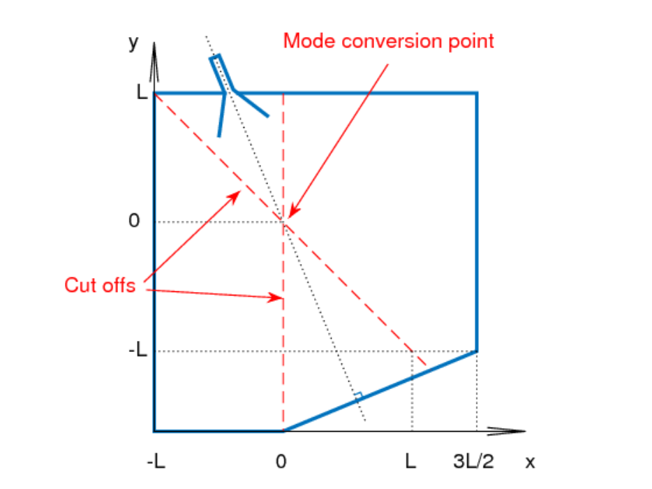
Then the antenna can be placed along any axis with an angle with respect to the axis, , as shown in Figure 5.

Along the main axis of the antenna, between the antenna and the mode conversion region, the zeroth order coefficient is constant on the antenna side and then varying as a quadratic function until the mode conversion point. It is odd as a function of t, the parameter describing the position along the steepest gradient line. Figure 5 also represents this coefficient along the main axis of the antenna, for different incident angles . The antenna is described by and , the parameter being negative between the antenna and the mode conversion point, and at the the mode conversion point.
The rest of the computational domain is a rectangle aligned with the and axis, except for the bottom right corner which is cut perpendicularly to the steepest gradient line . This cut is meant to avoid artificial reflections of waves outgoing from the transition zone toward the region.
The parameter in the boundary condition (31) determines the type of boundary condition. On the bottom wall of the antenna, an incoming plane wave, with wave length , is sent into the domain by a Robin type boundary condition, setting . On the other walls of the antenna, a perfect conductor type boundary condition is set by and . Absorbing boundary conditions are set on on all the other boundaries of the domain, setting and .
5.2 Results and comments
A series of results are proposed to illustrate the mode conversion phenomenon in the 2D model introduced in this work. Remember that by definition of the O- or X-mode cut-offs, a pure wave of the corresponding type can only propagate on one side of the cut-off. As a measure of mode conversion, define the transmission coefficient computed here as the relative difference between the maximum wave amplitude before the transition zone, i.e. on , and after the transition zone, i.e. on . All the following results were computed with basis functions per element, as the approximation order and with either or . The absolute value of the solution will always be represented with level curves. The transition lines between the constant and varying coefficient zones are indicated in blue. Note that the computational domain is meshed automatically by only imposing the mesh size, and so the mesh does not resolve the boundaries of the propagative and absorbing region, or the zones of constant and variable coefficients.
To present the type of results obtained, Figure 6 displays two solutions computed with the incident angle and , for both and . For the case, the antenna parameter is , the mesh is generated for a mesh size of , and is made of triangles. For the case, the antenna parameter is , the mesh is generated for a mesh size of , and is made of triangles. One can observe the same type of behavior: the outgoing wave propagates from the antenna, driven by the two cut-offs toward the mode conversion point. Reflection can be observed clearly in the transition zone where the coefficients are varying. Comparing these two solutions naturally suggests that the size of the transition zone plays an important role in the transmission process.


The transmission process is expected to depend strongly on the incident angle . Figure 7 displays this transmission coefficient as a function of the incident angle , for both and . Typical values of various geometry and mesh parameters used to produce Figure 7 are given in Table 1. As expected, the transmission is very low when is close to zero and , which correspond to launching the wave parallel one of the cut-offs, while a peak is observed between those two regimes, which corresponds to the wave propagation direction closer to the steepest gradient line of the variable coefficients. Figure 8 displays the solution with the maximum transmission as well as a solution completely reflected by the cut-off before reaching the mode conversion region.
| 6 | 7 | 8 | 9 | 10 | 11 | |
| 2.13 | 1.82 | 1.59 | 1.42 | 1.28 | 1.16 | |
| mesh size | 0.73 | 0.64 | 0.57 | 0.46 | 0.43 | 0.39 |
| number of triangles | 25157 | 36548 | 42412 | 60944 | 66511 | 78470 |

Figure 6 evidences the importance of the size of the transition zone on the mode conversion efficiency. Indeed the maximum transmission coefficient is a decreasing function of , which is a measure of the size of the transition zone. Moreover the size of the transition zone also influences the angle at which this maximum coefficient occurs. See Tables 2 and 3.
| 6 | 7 | 8 | 9 | 10 | 11 | |
|---|---|---|---|---|---|---|
| 3.49e-02 | 3.44e-02 | 3.18e-02 | 2.95e-02 | 2.48e-02 | 3.33e-02 | |
| 0.434 | 0.444 | 0.451 | 0.460 | 0.465 | 0.458 |
| 6 | 7 | 8 | 9 | 10 | 11 | |
|---|---|---|---|---|---|---|
| 6.50e-02 | 6.14e-02 | 6.09e-02 | 5.33e-02 | 4.57e-02 | 4.76e-02 | |
| 0.370 | 0.375 | 0.380 | 0.384 | 0.390 | 0.391 |
Acknowledgment
Many thanks to Harold Weitzner for introducing me to mode conversion and guiding me along the way, and to Jonathan Goodman for our many discussions. I also thank Teemu Luostari for providing his 2D PW-UWVF code for elasticity equations.
This work was supported in part by the U.S. Department of Energy, Office of Sci- ence, under Grant No. DE-FG02-86ER53223.
References
- [1] I. Babuska and S.A. Sauter, Is the pollution effect of the FEM avoidable for the Helmholtz’s equation considering high wave numbers? SIAM Rev. 42 (2000) 451–484
- [2] P.T. Bonoli Review of recent experimental and modeling progress in the lower hybrid range of frequencies at ITER relevant parameters AIP Conference Proceedings 1580 15–24 http://dx.doi.org/10.1063/1.4864497
- [3] P.T. Bonoli Electromagnetic mode conversion: understanding waves that suddenly change their nature Journal of Physics: Conference Series 16 (2005) 35–39
- [4] A. Buffa and P. Monk, Error estimates for the Ultra Weak Variational Formulation of the Helmholtz equation, ESAIM: Mathematical Modelling and Numerical Analysis42 (2008) 925–940
- [5] O. Cessenat, and B. Després, Application of an ultra weak variational formulation of elliptic PDEs to the two dimensional Helmholtz problem, SIAM J. Numer. Anal., vol. 55 (1998) 255–299
- [6] P. G. Ciarlet, The finite element method for elliptic problems. Studies in Mathematics and its Applications Vol. 4 (1978) North-Holland Publishing Co., Amsterdam-New York-Oxford.
- [7] Courant-Hilbert, Methods of mathematical physics. Vol. II: Partial differential equations. Interscience Publishers, New York-London 1962
- [8] B. Després, Sur une formulation variationnelle de type ultra-faible, C. R. Acad. Sci. Paris Sér. I Math. 318 (1994) 939–944.
- [9] C. Gittelson, R. Hiptmair and I. Perugia, Plane wave discontinuous Galerkin methods: analysis of the -version, M2AN Math. Model. Numer. Anal. 43 (2009) 297–331doi = http://dx.doi.org/10.1051/m2an/2009002,
- [10] R.A. Herman A Treatise on Geometrical Optics University Press, 1900
- [11] R. Hiptmair, A. Moiola, and I. Perugia, Plane wave discontinuous Galerkin methods for the 2D Helmholtz equation: analysis of the p-version, SIAM J. Numer. Anal. 49(2011) 264–284
- [12] T. Huttunen, M. Malinen and P. Monk, Solving Maxwell’s equations using the ultra weak variational formulation, Journal of Computational Physics, 223(2007) 731–758.
- [13] T. Huttunen, P. Monk and J.P.Kaipio, Computational Aspects of the Ultra-Weak Variational Formulation, Journal of Computational Physics 182(2002) 27–46.
- [14] L.-M. Imbert-Gerard, Interpolation properties of generalized plane waves coefficients Numerische Mathematik (2015) doi: 10.1007/s00211-015-0704-y
- [15] L.-M. Imbert-Gerard and B. Despres, A generalized plane-wave numerical method for smooth nonconstant coefficients IMA Journal of Numerical Analysis (2013) doi: 10.1093/imanum/drt030
- [16] H. P. Laqua, V. Erckmann, H. J. Hartfuß, H. Laqua, and W7-AS Team ECRH Group, Resonant and Nonresonant Electron Cyclotron Heating at Densities above the Plasma Cutoff by O-X-B Mode Conversion at the W7-As Stellarator, Phys. Rev. Lett. 78 (1997)
- [17] H. P. Laqua, H. J. Hartfuß, and W7-AS Team, Electron Bernstein Wave Emission from an Overdense Plasma at the W7-AS Stellarator, Phys. Rev. Lett. 81 (1998)
- [18] H. P. Laqua, H. Maassberg, N. B. Marushchenko, F. Volpe, A. Weller, and W. Kasparek (W7-AS Team, ECRH-Group), Electron-Bernstein-Wave Current Drive in an Overdense Plasma at the Wendelstein 7-AS Stellarator Phys. Rev. Lett. 90 (2003)
- [19] B. Pluymers, B. Hal, D. Vandepitte and W. Desmet, Trefftz-Based Methods for Time-Harmonic Acoustics, Archives of Computational Methods in Engineering 14 (2007) 343–381
- [20] J. Preinhaelter and V. Kopecký, Penetration of high-frequency waves into a weakly inhomogeneous magnetized plasma at oblique incidence and their transformation to Bernstein modes. Journal of Plasma Physics 10 (1973) 1-12 doi:10.1017/S0022377800007649
- [21] E. Trefftz Ein Gegenstück zum Ritzschen Verfahren, Proceedings of the 2nd international congress on applied mechanics, Zürich, Switzerland, (1926) 131–137
- [22] F. Volpe, Analytical solution of the O-X mode conversion problem, Physics Letters A 374 (2010) 1737–1741
- [23] H. Weitzner, Lower hybrid waves in the cold plasma model, Communications on Pure and Applied Mathematics 38 (1985) 919–932
- [24] H. Weitzner, O-X mode conversion in an axisymmetric plasma at electron cyclotron frequencies,Physics of Plasmas 11 (2004) 866–877
- [25] H. Weitzner and D.B. Batchelor, Conversion between cold plasma modes in an inhomogeneous plasma, Physics of Fluids 22 (1979) 1355–1358 http://dx.doi.org/10.1063/1.862747.