Drag phenomena from holographic massive gravity
Abstract
We consider the motion of point particles in a strongly coupled field theory with broken translation invariance. We obtain the energy and momentum loss rates and drag coefficients for a class of such particles by solving for the motion of classical strings in holographic massive gravity. At low temperatures compared to the graviton mass the behaviour of the string is controlled by the appearance of an exotic ground state with non-zero entropy at zero temperature. Additionally we find an upper bound on the diffusion constant for a collection of these particles which is saturated when the mass of the graviton goes to zero.
Holography is an extremely successful tool for computing physical observables in strongly coupled theories by considering weak perturbations of a gravity theory in one higher dimension [1, 2, 3]. Recently, increasing interest and efforts have been devoted towards modelling condensed matter systems in an attempt to learn about real world strongly coupled systems.
To more closely approach real materials incorporating momentum dissipation mechanisms in the gravity framework is essential. Without such mechanisms weakly coupled and holographic computations often lead to unrealistic results such as the divergence of the optical conductivity at zero frequency [4]. Several methods to introduce non-conservation of momentum have been proposed such as turning on a lattice distortion at the boundary (either through the modulation of the chemical potential or a scalar source) [5, 6, 7], the use of probe brane models [8, 9], helical lattices [10, 11], striped phases [12] and finally disorder [13].
An alternative method that has proven to be a very convenient way of incorporating momentum relaxation is the introduction of a graviton mass [14]. Following the original work many generalizations have been pursued with the common aim of having a complete description of strongly coupled metals, insulators and the transitions between them. For example, models with linearly sourced scalars were introduced in [15] and further developed in [16, 17, 18]. A slightly richer model than the linear scalar uses a dilaton field [19] while others have exploited global symmetries [20].
While the framework of massive gravity reproduces Drude peaks [21] and the metal-insulator transitions associated with broken translation invariance, the precise interpretation of the deformation in terms of which operators we turn on in the boundary theory is unclear. For example, in many condensed matter systems non-conservation of momentum can be associated with several phenomena such as the existence of phonons or the introduction of impurities. We shall find, by examining the heat capacity and the drag coefficient, that turning on a graviton mass cannot be uniquely identified with either of these condensed matter phenomena alone. Nonetheless we do see features generic to our large class of massive gravity models, in particular, a pronounced peak in the diffusion constant.
To try and illuminate the role of graviton mass we return to one of the simplest models in condensed matter theory: the Drude model. This describes the motion of a probe particle interacting with a medium. Generally a moving probe particle loses energy and momentum to the surrounding material leading to an effective viscous drag. In a weakly coupled theory momentum is typically lost by two body collisions and the production of massless particles via bremsstrahlung. Examining the drag coefficient can generically give clues as to which mechanism is dominant, what types of collisions are occuring and the nature of the emitted massless particles.
If the medium has broken translation invariance, either by the introduction of impurities or periodic potentials, we expect there to exist additional channels into which the probe particle can lose energy. It is important to note that the behaviour of phonons and impurities in a material are well understood in the condensed matter community. As such holographic studies investigating these phenomena are unlikely to yield new physics.
In [22, 23] a probe string is used to calculate the drag on a charged particle due to thermal Yang-Mills. The string is a probe of the spacetime and experiences momentum loss to the background without significantly affecting the latter’s energy. When the applied force is due to an electric field this is the holographic analogue of the Drude model. One endpoint of the string enters the black hole horizon, which describes the thermal state of the boundary field theory and acts to absorb energy and momentum supplied to the other endpoint. The second endpoint of the string in [22, 23] is attached to a D7-brane. One can compute the diffusion constant for quark flavour [23],
| (1) |
where is the ’t Hooft coupling, by considering the motion of the free string endpoint after it is given some initial impulse. In this paper we shall compute the diffusion constants for point particles in the field theories dual to holographic massive gravity noting that these are distinct from the charge diffusion constants typically considered [14, 16, 17, 10, 11, 12, 19, 20, 13].
We shall perform string drag calculations in a particular class of massive gravity models. To study the effect of momentum loss one would ideally like to study the motion of a string in the fully back-reacted spacetime dual to a boundary theory with a lattice. Doing this however requires a complex numerical calculation for the metric which obscures some of the physics. We could instead consider a model like that discussed in [24] which uses a weak scalar source in an Einstein-Maxwell-scalar theory to produce a modulated lattice. As was noted however the effect of this weak lattice is to give the graviton a mass precisely in the manner of [14]. Since we are interested in the generic features of drag with momentum loss we shall allow arbitrary potentials for the translation breaking scalars which encode generic massive gravity theories. Thus we are taking a bottom-up approach. No consistent UV completion of these frameworks is known so far and determining such a string embedding represents an important research programme.
As the physics we are interested in concerns IR features of the theory, knowing the UV stringy completion of our model is not necessary. It is very likely that a generic string theory embedding would contain more degrees of freedom, such as a dilaton field. We would expect the dilaton, which could couple to our Stuckelberg sector, to have a radial running. Non-conformality of the boundary theory and its consequences for the drag mechanism, due to the presence of homogeneous and isotropic (in the boundary theory directions) dilaton, have already been investigated in [25]. Its effects in the context of holographic theories with momentum dissipation have also been determined [19, 26, 20, 27]. In particular, a strong dilaton can greatly modify the IR solutions of the system leading to new (often insulating and gapped) phases of matter. In order to separate the consequences of breaking translational invariance from those due to the running couplings, whose effect we already know, we have assumed that the background dilaton is vanishing.
We begin the paper by discussing the theory of drag and its relevance to the Drude model of charge transport. Subsequently we give a brief description of one model of massive gravity and discuss contributions to the heat capacity at constant volume. We then compute the drag coefficient and energy/momentum loss rates to the horizon for a probe string. At low temperatures with respect to the graviton mass we find that these observables are controlled by the formation of an exotic ground state with non-zero entropy at zero temperature. Our results also indicate the existence of an upper bound on the diffusion constant of a collection of the probe particles.
1 The theory of drag
Consider a particle moving with spatial momentum in a viscous medium under a driving force . We model the motion of this particle using the drag equation
| (2) |
where is called the drag coefficient. We shall generally examine situations where the speed of the particle is low enough that its motion can be considered non-relativistic so that the dispersion relation takes the form
| (3) |
where is the temperature of the medium. In this case we define the spatial momentum to be and for steady state behaviour at constant velocity we find . We are particularly interested in determining the drag coefficient of this particle.
Observing the stationary velocity the particle achieves under an applied force allows us to determine the combination . Moreover if we assume the particle is charged and the applied force is due to an electric field then (2) is exactly the Drude model. The DC conductivity11 1 In holographic theories with a charge sector can be shown to consist of two terms [19]: (4) The first term is due to quantum pair creation and can be non-zero at zero charge density. It corresponds to the conformal part of the conductivity. The second contribution is due to dissipative mechanisms and its value in the Drude model studied in undergraduate condensed matter courses is given by (5). of the Drude model is well known,
| (5) |
where is called the relaxation time, is the unit of fundamental charge and is the density of charge carriers. To obtain we then consider the late time unforced behaviour of the particle with some initial momentum and solve the drag equation (2) to find
| (6) |
A measurement of the ratio will then allow us to determine and subsequently .
Moreover, if the force in (2) contains a random element we can consider the Brownian motion of the particle through the medium. Under suitable assumptions on the nature of the statistical force it can be shown that the diffusion constant is given by (which is called the Einstein relation). Once again if the particle has charge and we place it in an external electric field it will accelerate. At late times the velocity of that particle is . Defining the mobility by we find
| (7) |
which is called the Nernst-Einstein relation. We shall use this expression later on to determine the diffusion constant of probe particles moving in a strongly coupled field theory assuming that the statistical force supplied by fluctuations of the black hole horizon satisfies the conditions necessary for (7) to apply. See [28] for further discussion.
2 Holographic massive gravity
We use a generalised model of massive gravity to supply the background upon which our string moves. This is inspired by [17] where massive gravity is realized in a fully covariant formalism through the explicit introduction of Stueckelberg fields. This is convenient in order to have easy control on the number of degrees of freedom and possible inconsistency issues for which we refer to [29]. The minimal covariantization in the present case requires a set of scalar fields transforming under an internal Euclidean group of translations and rotations in field-space (for further details about this procedure see [30]). Our massive gravity action is then recovered by a truncation to 2-derivative operators:
| (8) |
with some polynomial. This theory admits solutions where the scalars take on linear expectation values with the Kronecker delta22 2 This choice leaves the Ward identity for energy conservation unbroken while breaking spatial translation invariance.. On these solutions the mass matrix for the graviton is identified as . Note that the Lagrangian for the scalars has some similarities with the effective Lagrangian describing phonons [31, 32]. It is necessary for to be monotonically increasing in to avoid ghosts and we choose so that asymptotically AdS spaces are a solution when the scalars vanish.
As the Einstein equations are easy to derive we shall not present them here. A class of metrics which solve these equations are of the form
| (9) |
where , for general potential , reads:
| (10) |
with being related to some coupling between the scalars. For monomial choices of one of the parameters, or , is redundant and can be reabsorbed via an appropiate redefinition. For polynomial both the parameters are independent and can play a different role. Henceforth we set .
Considering (10) it can be seen that at we have a coordinate singularity. Despite the known potential issues of singularities in the context of black holes geometries in massive gravity theories [33], our solution seems to be totally healthy and smooth. This is because in our scenario the Stueckelberg fields have non trivial profiles only in the spatial directions as compared to the Lorentz invariant case discussed in [33]. Therefore the invariant object is regular at and we do not need to concern ourselves with the remedy to these problems described in [33]. Another quick, but non-comprehensive test, is to consider the standard curvature invariants , and which all remain finite at .
As all the emblackening factors of (10) have a zero at , where there is no curvature singularity, our spacetime can be interpreted as thermal with a temperature given by:
| (11) |
To obtain this temperature we follow the standard procedure of continuing to Euclidean time and imposing smoothness of the manifold at through suitable periodicity conditions. This ensures that correlation functions on the boundary share this property, the hallmark of a thermal field theory.
We can see from (11) that it is possible to set at non-zero and have extremal black holes. It is worth noting that the non-trivial scalars, in particular , enter the first law like a magnetic field [15] (or conversely a charge in four spacetime dimensions). As a consequence it is not surprising that one can reach an extremal limit by dialing the graviton mass appropriately as the scalar hair will support the black hole. Indeed assuming that the entropy density is given by the area of the black hole horizon we find
| (12) |
which is non-zero at zero temperature if there is a non-trivial solution to (11). The entropy density is also displayed in fig. 1 for vanishing graviton mass and an example potential . Indeed, for all but a few special cases where the emblackening factor has higher order degeneracies at the extremal IR geometry turns out to be ; typical of extremal black holes. It would be interesting to study such IR extremal geometries and their instabilities.
With the above remarks about the thermodynamics in mind we note that the position of the black hole horizon can be given as a function of the temperature and graviton mass by solving
| (13) |
for . This is bounded above by the zero graviton mass result33 3 To see this assume that both and must be positive (the possibility of having negative temperature goes beyond the scope of this paper). Thus, when this equation has a solution it must be the case that the quantity in square brackets is positive. Moreover because is monotonically increasing between zero and (to avoid ghosts) and (so asymptoticlly AdS spacetimes are a solution) the same term is bounded above by one. It equals one only when the second term is zero (for example when the graviton mass is zero). Thus proving the result.. For the square root () and linear () potentials, upon solving (13) for , we find the simple and exact results:
While there is no such simple result for higher power monomial potentials, generically we see that for larger powers of in the leading correction to the zero graviton mass result is smaller. At large temperatures () we can show that the leading correction to the zero graviton mass horizon position is
| (17) | |||||
| (18) |
where we have assumed the leading term in the potential at small is proportional to . Thus if then we can ignore the effect of graviton mass and our spacetime is thermal AdS.
At low temperatures we face an obstruction to determining in terms of small , namely the massive gravity spacetimes potentially exhibit zero temperature black holes with given by the smallest real solution to
| (19) |
These black holes are interesting and particularly worthy of independent study. We note that (19) always has a real solution if and is monotonically increasing. Let be the smallest real solution to (19). For the square root and linear potentials this is given by
For any potential we find the horizon position as a function of small is given by
| (23) |
The above asymptotic expansions for the horizon position at small and large temperature, (23) and (17) respectively, will be particularly useful for determining the behaviour of the drag coefficient and momentum loss rates at the relevant extremes.
There are of course many possible potentials we could consider here. We will often consider , the monomial potentials44 4 We have found that the features of generic potentials can often be identified from the features of the monomial potentials. We shall see that the smallest power of in is almost always dominant at large temperatures and small . In the opposite regime it is often the largest power of that dominates. The interest in non-linear combinations, such as comes from the fact that they give rise to metal-insulator transitions [17]., with . The choices and are due to the existence of the exact and simple results given in (2) and (2). For larger we are forced to use numerics exclusively but will also use these techniques for as the analytic results are not concise. For intuitive purposes we will consider , with some positive real number, where appropriate.
2.1 The heat capacity
For fixed potentials there are two thermodynamic state variables in our background - volume and temperature. We expect the thermodynamic potential to be extensive in volume and thus we can drop the former leaving only a single scale - the temperature - to be concerned with. The response of the system to thermodynamic forces is encoded in the susceptibilities and for us in particular the volumetric heat capacity at constant volume,
| (24) |
where is the entropy density of the system defined in (12). We note that for thermal AdS, i.e. , the heat capacity at constant volume is
| (25) |
In a typical material there can be several contributions to the heat capacity coming from distinct fields, for example, charged impurities55 5 Generically uncharged impurities do not contribute to the heat capacity. and phonon excitations. We now examine the behaviour of this quantity for various potentials to ensure the thermodynamic stability of our background.
Consider the monomial potentials . The heat capacities are displayed in fig. 2. We can see that for the zero graviton mass result, (25), as the temperature goes to zero the heat capacity vanishes. This remains true for non-zero graviton mass (left-hand plot of fig. 2) and the heat capacity is positive and at low temperatures. Thus the system, governed by the exotic ground states with non-zero entropy density, is at least locally stable to thermodynamic fluctuations at low temperatures [34]. This does not guarantee of course that it is stable to other types of fluctuations nor that we have a global thermodynamic minimum. See [35] for a general discussion of the thermodynamics of black holes in massive gravity.
From the left plot of fig. 2 we can see that for the linear potential there is something like a saturation temperature where the effect of the graviton mass is largest. It may be tempting to interpret this as a Debye temperature. However, we note that while calculating the difference between the heat capacity at zero and non-zero graviton mass certainly captures the change in this quantity due to spatial translation symmetry breaking it is difficult to argue that the additional heat capacity is due to the introduction of a new species, such as phonons, alone.
Higher monomial and polynomial potentials have heat capacities that are reduced from the vanishing graviton mass value over some intermediate range of temperature (fig. 2 bottom right and top left). Naïvely one would expect the addition of extra modes to increase heat capacity. This result suggests that some of the entities that contribute to the zero graviton mass heat capacity require more energy to excite as the graviton mass is increased. This would offset the introduction of more modes and lead to the reduced heat capacity observed.
For square root and linear potentials the heat capacity can be expressed analytically as
At large temperatures compared to we find the difference in the heat capacity from its zero graviton mass value (25) is
| (29) |
except when where the next to subleading term must be considered. It is clear that for at large temperature the change in the heat capacity increases with increasing temperature. When however the opposite is true. This can clearly be seen in the left plot of fig. 2. This expression confirms for large temperatures that the correction to the zero graviton mass result is negative when and positive when .
Importantly, for the monomial potentials we consider and , with appropriate choices of , the total heat capacity is positive and grows with temperature in the range of temperatures and examined. Thus our background is at least locally stable to thermal fluctuations.
3 Motion of a string in holographic massive gravity
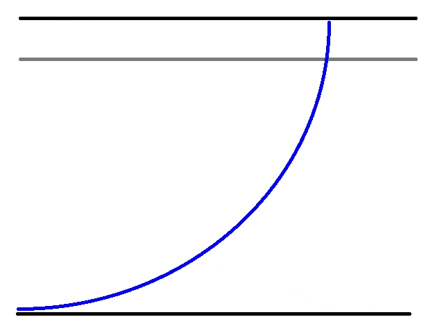
Now that we have discussed the background we turn to calculating the motion of a string in it. We wish to consider a string dangling into the black hole horizon with the other end fixed to a constant hyperplace (see fig. 3). We shall assume that the translation breaking scalars only affect the string through the pullback of the bulk metric to the worldsheet. Thus the string action is just
| (30) |
where is the string tension, are the embedding scalars and are the worldsheet coordinates. The equations of motion for the string take the form
| (31) |
where , are given by varying the Lagrangian density with respect to and respectively. Assuming the string action takes the form (30) may be inconsistent if we attempt to embed (8) in string theory but as an exercise this allows us to isolate how much the change in the background metric from thermal AdS affects the string and subsequently the drag on the point particle.
We shall always choose static gauge , and let the only non-trivial string profile be . The Lagrangian density is
| (32) |
and the canonical momenta are
The equations of motion for the string worldsheet embedding are
| (47) |
with the outgoing boundary condition at and where the string is subject a force on the constant surface. We note in [23] that this force is supplied by a constant electric field on a -brane whose embedding terminates at due to the finite quark mass. Here we shall assume the force can be supplied by some mechanism and remain agnostic about its origin.
3.1 The low velocity dispersion relation
Generically we shall choose the string endpoint not dangling into the horizon to move at small velocities. This allows us to extract analytically the form of the dispersion relation. In this section we shall argue that it takes the non-relativistic form independent of the string length. Firstly we calculate the static energy of the string. Choosing the string to sit at a constant value of solves (62) and gives a total static energy
| (48) |
The momentum of this static string is zero. While the expression for the static energy (48) in terms of the horizon position and string endpoint is the same as that found for thermal AdS [22, 23] we note that the dependence of on temperature, through , is different.
Now consider a string imparted with some initial momentum and allowed to relax. At very late times the drag on the string will make it static. Prior to this point we can consider it as having some small velocity which deforms the string from the static profile. Such an embedding can be described by , where is a parameter of smallness, and the equation of motion for the fluctuation becomes
| (49) |
Solving for the fluctuation and using (3), which we do in appendix A, it is possible to determine the dispersion relation at low velocities. For ease we repeat the result, (94), here
| (50) |
with given by (48). The quantity defined above is the mobility of (7). To produce this result we have assumed that the velocity of the string endpoint is given by , at late times, with the as yet undetermined drag coefficient. We shall compute in section 3.3 and thus show that this assumption is valid at late times.
It is important to note before moving on that the mobility of (50) is inversely proportional to the entropy density of the field theory. Given that the entropy density increases for non-zero potential (see right plot of fig. 1 for example) the decreased mobility of fig. 4, for non-vanishing potentials, is consistent with the interpretation of broken translation invariance in the boundary theory. The reason for this is that when we remove the requirement that microstates of the system must preserve spatial translation invariance the number of allowed states increases and there are more channels by which the particle can lose momentum.
Although the graviton mass and potential enter in the definition of quantities like the entropy and energy there is a single thermodynamic parameter for the background - the temperature - once we fix the potential. Thus we should compare the mobilities in theories with the same temperature normalised by .
Due to the bound on the temperature defined by (13), the mobility is bounded above by
| (51) |
The expression for zero graviton mass is equal to , displayed in (51). For the square root and linear potentials, using (2), we find
These and more general results for the mobility with various choices of the free parameters are displayed against temperature in fig. 4. We see that the mobility generically decreases with increasing and decreasing temperature. For all potentials we see that for low values of with respect to , on applying (17),
| (55) |
where the leading power of in at small is assumed to be proportional to . From (55) it is also clear that the higher the power of in the weaker the correction to the case of zero graviton mass. We have observed that the situation switches at large with respect to . Monotonicity of the potential with these two results is then sufficient to indicate the existence of a value of where any pair of mobilities will have the same value (see left plot of fig. 4). For the monomial potentials66 6 The mobility can be used to partially classify the potentials . Consider where is a polynomial in . The horizon position can be determined by solving (56) As we noted earlier, by the monotonicity property of the potential and assuming that at large larger powers of give greater corrections to the zero graviton mass result, there must be a crossing point for any two potentials. In particular consider and . Because the right hand side of the above equation is independent of it must be the case that (57) The crossing point is given by solving this equation and is independent of . Thus all the potentials of the form have a fixed value of the mobility at some value of . this happens when . It would be interesting to understand whether the existence of this point has some physical implications such as enhanced symmetries.
From (7) and (50) we can additionally determine the diffusion constant for a collection of string endpoints which has the form
| (58) |
Examples of the diffusion constant are displayed in 5. Except for the case of vanishing potential there is a peak in the diffusion constant at some value of temperature which moves to larger temperature as the power of the monomial increases. It is also interesting to notice that the diffusion constant goes to zero at in the case of non-zero graviton mass where the exotic ground state is formed.
Moreover, because the mobility is bounded above by the zero graviton mass result the diffusion constant is also bounded above by its zero graviton mass value. The existence of this upper bound is deeply related to the fact that is monotonically increasing (no ghosts) and that (asymptotically AdS spaces are a solution to the background equations of motion). A naïve argument of what should happen to the diffusion constant in the presence of broken translation invariance would be that breaking a symmetry permits previously forbidden processes. We expect these to contibute positively to dissipation and thus the diffusion constant to increase. Clearly this cannot be correct alone and the results displayed in fig. 5 are consistent with the idea that there is an increased energy gap for processes that contribute to dissipation. This naturally makes the interpretation of our results in terms of new processes, like phonon production or interaction with impurities, more difficult because the change in the diffusion constant, drag coefficient and so on cannot be attributed to such a process alone.
Were the reader to have picked up the paper at this point they may be a little surprised as the famous result for thermal transport in holographic systems places a lower bound on the diffusion constant. A bound for diffusion in strongly interacting systems with charge was recently proposed in [36] which our system violates badly at sufficiently small temperatures with respect to . See [37] for another model which possibly violates this bound. If we are to accept that the conjectured bound of [36] is indeed universal this perhaps suggests an instability in our system at low temperatures. To help decide which, if either, solution is correct it is necessary to better understand the interpretation of the string in the field theory dual to massive gravity spacetimes.
We note in passing that many of the dynamical properties of a collection of particles are related to the mobility. It would be interesting to understand whether there are consequences of our bound for other transport quantities such as the thermo-electric transport coefficient recently investigated in [38, 39] for duals to massive gravity.
3.2 Steady state motion at constant velocity
For completeness we shall work at arbitrary velocity initially and only take the low velocity limit at the end of the calculation. We consider the following ansatz for the string profile
| (59) |
which describes a particle moving at constant velocity in the direction on each constant -plane. We substitute (59) into the equations of motion (62) and solve for taking the string to stretch from the horizon to the boundary (). We must impose a force on the string equal to the momentum loss rate to achieve steady state behaviour. Shorter string profiles, where , can then be found by slicing the profile of the “full” string.
The Lagrangian of (32), assuming (59), becomes
| (60) |
From this expression it is clear that is a cyclic coordinate so we define
| (61) |
where is a constant. This expression can be inverted to give a first order differential equation for ,
| (62) |
where the sign is fixed to by requiring the string to trail behind the free endpoint. We note that because interpolates monotonically between zero and one and there is a value of where changes sign. If the string turns over at this point and returns to the boundary then this is not a problem. However the situation with two string endpoints terminating on the boundary describes a pair of interacting particles. For a single particle the string must past through the black hole horizon and thus the denominator must change sign at the same point (lest the induced metric of the string not be real). As such we must find solutions to the equation
| (63) |
and set .
When the spacetime is thermal AdS it is straightforward to solve (63) to find
| (64) |
However there are corrections for the massive gravity spacetimes and solving (63) will generically require a numerical approach. In the case of small velocities we can however determine that
| (65) |
and thus
| (66) |
It is sufficient to know from solving (63) to determine the energy and momentum loss rates. Substituting our profile (59) into (61) we see that . Thus is constant along the string following (31). Hence we can evaluate at any point on the string including at the horizon. Using (61) we can thus determine the loss rates to be
| (67) |
respectively. In the low velocity limit the momentum loss rate becomes
| (68) |
It is important to now clarify that there is non-zero energy loss for the string even in the case of non-zero graviton mass due to the probe limit. The way that linear sources for our scalars were chosen in (8) means we are only breaking the subgroup of the full Lorentz symmetry responsible for momentum conservation. The Ward identity for the time component is kept untouched and energy is a completely conserved quantity in the background theory.
For the square root and linear potentials we can determine the momentum loss rate analytically as is at most quadratic in . Only the linear potential has a compact form however which we display for posterity
| (69) | |||||
| (70) |
Noting that enters as a square we see that only for quite relativistic velocities is there a signficant difference from the result. We display the momentum loss for generic potentials in fig. 6. Beginning with the linear potential in the left plot we see that at large temperatures the momentum loss tends to the same large behaviour i.e. . This large behaviour is the same as the momentum loss of the zero graviton mass case,
| (71) |
which is sensible because the effect of graviton mass is reduced by large temperature. At small temperatures however there is a non-vanishing momentum loss for non-zero graviton mass unlike in the case of zero graviton mass. Gravitationally this is because there are non-trivial solutions to (19) for the linear potential. In terms of the field theory we can see that the entropy density is non-zero at zero temperature. Thus there are states that the point particle can lose energy and momentum to.
The other monomial potentials follow the same generic pattern. At large temperatures and small we find that the momentum loss tends to (71). At the opposite extreme we find that the formation of the zero temperature black holes leads to a momentum loss approximately independent of temperature. Physically there is a non-zero density of states for the string to radiate momentum to at zero temperature as indicated by the non-zero entropy density. Again, we can understand this from the gravity side by solving for the position of the horizon at zero temperature
| (72) |
As the power of the monomial potential increases the momentum loss at small temperatures increases (see top-left of fig. 6). Finally, from the physical point of view, increasing the power in the monomial potential should increase the strength of the interactions responsible for momentum dissipation and therefore increase the momentum loss itself. This can be seen from the bottom plot in fig. 6.
On the condition that the velocity is small the momentum loss has the following generic behaviour
| (73) |
where again is the entropy density. This is a lower bound for the momentum loss in the velocity as for non-zero we see that . Unsurprisingly the momentum loss increases as the velocity increases. The approximate relation for the momentum loss (73) at small velocity also indicates that for as increases the momentum loss increases while for it decreases. This can be seen in fig. 6 where the zero temperature momentum loss increases with increasing .
Having computed the value of the embedding equation (62) must generically be numerically integrated to determine . At small we see from (62) that
| (74) |
and thus we require that is a constant. Subsequently we can integrate (62) to determine the string profile
| (75) |
which we display in fig. 7. To describe a string stretching from a constant -surface, , to the horizon that starts at at we simply slice our embedding and use the coordinate shift
| (76) |
As we noted the canonical momenta along the string do not vanish. Following [22, 23] a force must be applied to the string endpoint at so that we cancel the momentum loss and subsequently satisfy the variational principle. Setting the force equal to the momentum loss rate and substituting into the force balance equation yields
| (77) |
where here indicates the usual dot product and we have assumed low velocities so that . We see that the expression for to the lowest order in matches that given in (50).
3.3 Late time unforced motion
Earlier, in section 3.1, we described the behaviour of a particle at late times but neglected to determine the decay constant as this required a numerical quasi-normal mode analysis. We now seek to remedy this omission. Using the Fourier decomposition of (89) and substituting into (49) leads to
| (78) |
We will solve this equation numerically for the lowest quasi-normal mode as a function of the temperature and by imposing outgoing conditions on the past horizon and then searching for such that at some choice of . There are also two regimes where we can find analytic results to compare against these numerics: small and large static energies.
Before performing this analysis we note that our major results so far (namely the mobility and momentum loss rates) in sections 3.1 and 3.2 were independent of the string length. However the drag coefficient is dependent on this quantity. We have already argued we should compare theories of massive gravity at the same temperature. Now we make the choice to compare strings in those theories with the same static energy (48). For a choice of mass and potential picking the temperature amounts to fixing . Comparing strings of the same static energy then fixes . Thus the free parameters are the temperature , static energy , and the potential.
We display the results of numerical computations of the drag coefficient for various potentials in fig. 8 and fig. 9. We begin first with vanishing graviton mass summarising the results of [22, 23]. For small static energies the decay constant of the string is linear in the temperature and independent of ,
| (79) |
For large static energies the decay constant is
| (80) |
On fixing the temperature and varying the static energy we see in the top left plot of fig. 8 a smooth interpolation between a constant and behaviour at small and large respectively.
Turning now to the linear potential, in the bottom plot of fig. 8 we display the drag coefficient for various values of the graviton mass, with , against temperature normalised by the zero graviton mass result. The difference is always positive indicating that there is an increased drag when the graviton mass is non-zero. As expected when the temperature increases this effect diminishes as the spacetime begins to resemble thermal AdS. When the temperature is small with respect to both and we find that the drag coefficient tends to a constant. It then increases with increasing temperature before peaking and subsequently decaying in a manner consistent with the high temperature result. In the top right plot of fig. 8 we can see that as increases the drag coefficient also increases. The amount that the drag coefficient grows by is dependent upon the static energy of the string with smaller energies and larger energies being less affected by the graviton mass.
In the top right plot of fig. 9 we display the drag coefficient for various potentials against . Again we see that as increases the drag coefficient also increases. When vanishes we get the zero graviton mass value for the drag coefficient which is generally dependent on the static energy and the temperature. For small values of the larger the power of the monomial potential the larger the drag coefficient. This switches at some finite value of so that potentials with greater powers have smaller drag coefficients.
From the top left plot of fig. 9 we also note that at large or small the dependence of the drag coefficient on the potential diminishes just as was seen in the top right plot of fig. 8. In the bottom left plot of fig. 9 we another generic feature of the drag coefficient - a peak in the temperature. It is interesting that the existence of this peak is a generic fingerprint of the model which does not rely strongly upon the choice of a particular potential. Additionally, for sufficiently large temperature, the difference in the drag coefficient scales as (where is the power of the monomial potential) as shown in bottom-right of 9.
Having discussed our numerical results we would like to interpret them. For small static energies at non-zero temperature we use the analytic results of appendix B, namely (96), to show that graviton mass has no effect on the decay constant. This is consistent with the top right and top left plots in fig. 8 and with going to zero for small in the top left plot of fig. 9. In terms of the gravity theory this is unsurprising because the near horizon geometry of (9) takes the same form for both thermal AdS and all our massive gravity spacetimes at non-zero temperature. The interpretation in the field theory is also relatively straightforward - namely the static energy is much less than the average thermal energy and thus the string is excited to the average thermal energy independent of the small differences in mass.
For small and large static energies we use (101) to find
Clearly in the limit of large temperatures compared to , where the graviton mass becomes negligible, this reproduces (79) and (80). More generally, for , where the behaviour of the mobility is displayed for various potentials in fig. 4. As we noted the mobility is bounded above at fixed temperature by the zero graviton mass result and is a decaying function as is increased and temperature decreased. Similarly therefore the decay constant of strings with large static energies is bounded below at fixed temperature and generically increases with decreasing and increasing temperature.
For completeness we also determine the effective kinetic mass. In the limits of small and large static energy it has the analytic form:
This is compared to numerics in fig. 10. The left-hand plot shows the dependence of the effective kinetic mass upon the static energy for the linear potential at various temperatures and fixed . It is clear that as the static energy is increased we get the linear result given in (3.3). As the temperature is increased in the limit of small static energies the effect of is diminished and we get the analytic result
| (87) |
This can be seen in the left hand plot of fig. 10 by the fact that for large temperature the brown lines at small have approximately linear spacing. The right hand plot of fig. 10 shows the effect of varying for the monomial potentials at fixed and . Above some value of the larger the power in the monomial, the larger the effective mass. Because we have chosen a relatively large compared to the temperature as is taken to zero the monomial potentials have a kinetic mass which is almost equal to the kinetic mass of the string at vanishing graviton mass.
4 Conclusions
| Broken translation invariance | Unbroken translation invariance | |||
| - | - | |||
| - | - | |||
We have calculated the momentum loss rates of probe strings in various solutions to a particular, very general, model of massive gravity. We have found that the mobility and subsequently the diffusion constant of the dual point particles is bounded above by the zero graviton mass result. Moreover we have extracted the contribution of the graviton mass to the decay rate of a particle given some initial impulse. These results are summarised in table 1.
We have argued that at low temperatures the behaviour of the string is governed by the existence of a set of non-trivial ground states. This is of course predicated on the idea that these ground states, which have non-zero entropy density at zero temperature, are stable. However, it is known that often such states are unstable. As these new ground states are quite exotic they are worthy of independent study which would simultaneously determine whether we can trust our results at low temperatures.
We have seen that it is not possible to assign the additional momentum loss felt by a probe particle in field theories dual to massive gravity to a unique condensed matter phenomenon such as phonons or impurities. Our work thus indicates that extreme caution must be employed when using condensed matter terminology to describe the outcome of holographic experiments with massive gravity spacetimes. However, it has been argued [24] that a small graviton mass can be generated by a weak lattice in a gravitational version of the Higgs’ mechanism. Understanding the relationship between a probe string moving in a background with a non-weak lattice and the subsequent effective massive gravity theory should in principle help to clarify the role of different mechanisms, such as phonon production and interactions with impurities, responsible for the additional momentum loss observed in this paper.
Finally, we made the simplifying assumption that our classical string was uncharged under the scalar fields. If the total action given by the sum of (8) and the string action is to preserve the shift symmetry , so that we can treat the -fields as Goldstone bosons for broken translation invariance, the action of the string can have the more general form
| (88) |
where and are two unknown functions of . The function describes how the string is charged under the fields while describes some effective tension. It is also possible to add a Fradkin-Tseytlin term to the action77 7 We thank the anonymous reviewers for pointing out that such a term could have non-trivial effects.. Such a term would couple any non-trivial background dilaton to the worldsheet curvature and significantly complicate the equations of motion. As we have assumed that the background dilaton vanishes we have not worried about such a term. Even in the presence of a non trivial dilaton profile however two comments are in order: firstly, the Fradkin-Tseytlin term would probably be an correction, which is certainly interesting but beyond the scope of the present paper. Secondly it is not clear from the holographic point of view whether such a term contributes to the on-shell action or whether it represents a pure counterterm88 8 We would like to thank E. Kiritsis for discussions on this point.. That said, it would certainly be interesting to understand the effects of such a term.
It may be interesting to ask how the physics changes when dependence on the scalar fields enters through more than the pullback of the bulk metric. We still expect to see non-zero momentum loss at zero temperature, if only due to the interaction of the string with the background scalars, although it is unclear to us whether our bound on the diffusion constant should survive. Moreover, it may be possible to motivate from a string model an effective field theory where the string is charged under the translation breaking scalars using methods similar to [24]. This would allow a precise interpretation of the string in terms of the boundary field theory as well as providing explicit forms for the undetermined functions in our string action.
Acknowledgements.
MB acknowledges support from MINECO under grant FPA2011-25948, DURSI under grant 2014SGR1450 and Centro de Excelencia Severo Ochoa program, grant SEV-2012- 0234. DB is supported by the Israeli Science Foundation (ISF) 392/09 and a Fine Fellowship. We would like to thank Oren Bergman, Mike Blake, Alessandro Braggio, Mikhail Goykhman, E. Kiritsis, Oriol Pujolás and Amos Yarom for reading early drafts and offering various insights into the problems presented here. MB would additionally like to thank Federico Caglieris, Giacomo Dolcetto, Francesca Telesio and Genis Torrents for useful conversations and comments.Appendix A Analytic results for the mobility
Consider the fluctuation equation (49). Shifting to Fourier space with the conventions,
| (89) |
we find the spatial momentum of the slow string is
| (90) |
where we have regulated the momentum in the IR with an explicit cut-off which in principle we should take to be . Satisfying the outgoing condition at the past horizon requires as . Integrating against frequency we see
| (91) |
Turning now to the energy density of the string,
| (92) |
and integrating against the string length we find the total energy of the string is equal to
| (93) |
where we have imposed the outgoing condition as .
If the free string endpoint is to satisfy the drag equation (2) it must be the case that . Using the low velocity limit and integrating the velocity against time implies up to an additive constant we set to zero. Substituting into (93) then gives
| (94) |
with given by (48).We have yet to show that we can arrange for the endpoint to move according to , and determine the drag coefficient , which we shall do this in section 3.3.
Appendix B Analytic results for the decay constant
We can extract some analytical behaviour for our drag coefficients in the regimes of small and large static energies. Beginning with the former we solve the fluctuation equation (78) in a near horizon expansion and find the derivative of the fluctuation is
where
| (95) |
Setting imposes a constraint on the frequency and we find
| (96) |
This is the same result one finds for a short string in thermal AdS [22, 23].
A second regime where we can find an analytic solution to compare with the numerics is the long string. To solve the fluctuation equation (78) assume that we can perform a small frequency expansion for non-trivial ,
| (97) |
We will find that non-trivial solutions exist only when is of order with . We impose the outgoing condition on the past horizon and use an overall scaling of the linerised fluctuation equations
| (98) | |||||
to set
| (99) |
Solving the equations (98) up to second order in and calculating the derivative at we find (logarithmic term is not quite right)
| (100) | |||||
It is clear that for a non-trivial solution we cannot truncate to order but must cancel the order and terms. Expanding the Neumann condition to leading order in small we see find
| (101) |
This is small, as required by our expansion (97), on the condition that the string is long i.e. .
We see that the long string has fixed dependence on and as long as the line element has the form (9). The dependence on and is the same as that found by [22, 23]. However, once again, because depends on the temperature and graviton mass the drag coefficient of long strings is distinct between different theories of massive gravity at the same temperature.
References
- (1) J. M. Maldacena, The Large N limit of superconformal field theories and supergravity, Int.J.Theor.Phys. 38 (1999) 1113–1133, [hep-th/9711200].
- (2) S. Gubser, I. R. Klebanov, and A. M. Polyakov, Gauge theory correlators from noncritical string theory, Phys.Lett. B428 (1998) 105–114, [hep-th/9802109].
- (3) E. Witten, Anti-de Sitter space and holography, Adv.Theor.Math.Phys. 2 (1998) 253–291, [hep-th/9802150].
- (4) S. A. Hartnoll, Lectures on holographic methods for condensed matter physics, Class.Quant.Grav. 26 (2009) 224002, [arXiv:0903.3246].
- (5) G. T. Horowitz, J. E. Santos, and D. Tong, Optical Conductivity with Holographic Lattices, JHEP 1207 (2012) 168, [arXiv:1204.0519].
- (6) G. T. Horowitz, J. E. Santos, and D. Tong, Further Evidence for Lattice-Induced Scaling, JHEP 1211 (2012) 102, [arXiv:1209.1098].
- (7) P. Chesler, A. Lucas, and S. Sachdev, Conformal field theories in a periodic potential: results from holography and field theory, Phys.Rev. D89 (2014), no. 2 026005, [arXiv:1308.0329].
- (8) A. Karch and A. O’Bannon, Metallic AdS/CFT, JHEP 0709 (2007) 024, [arXiv:0705.3870].
- (9) S. A. Hartnoll, J. Polchinski, E. Silverstein, and D. Tong, Towards strange metallic holography, JHEP 1004 (2010) 120, [arXiv:0912.1061].
- (10) A. Donos, B. Goutéraux, and E. Kiritsis, Holographic Metals and Insulators with Helical Symmetry, JHEP 1409 (2014) 038, [arXiv:1406.6351].
- (11) A. Donos, J. P. Gauntlett, and C. Pantelidou, Conformal field theories in with a helical twist, arXiv:1412.3446.
- (12) Y. Ling, P. Liu, C. Niu, J.-P. Wu, and Z.-Y. Xian, Holographic Superconductor on Q-lattice, JHEP 1502 (2015) 059, [arXiv:1410.6761].
- (13) A. Lucas, S. Sachdev, and K. Schalm, Scale-invariant hyperscaling-violating holographic theories and the resistivity of strange metals with random-field disorder, Phys.Rev. D89 (2014), no. 6 066018, [arXiv:1401.7993].
- (14) D. Vegh, Holography without translational symmetry, arXiv:1301.0537.
- (15) T. Andrade and B. Withers, A simple holographic model of momentum relaxation, JHEP 1405 (2014) 101, [arXiv:1311.5157].
- (16) M. Taylor and W. Woodhead, Inhomogeneity simplified, Eur.Phys.J. C74 (2014), no. 12 3176, [arXiv:1406.4870].
- (17) M. Baggioli and O. Pujolas, Holographic Polarons, the Metal-Insulator Transition and Massive Gravity, arXiv:1411.1003.
- (18) M. Baggioli and M. Goykhman, Phases of holographic superconductors with broken translational symmetry, arXiv:1504.0556.
- (19) B. Goutéraux, Charge transport in holography with momentum dissipation, JHEP 1404 (2014) 181, [arXiv:1401.5436].
- (20) A. Donos and J. P. Gauntlett, Holographic Q-lattices, JHEP 1404 (2014) 040, [arXiv:1311.3292].
- (21) M. Blake and D. Tong, Universal Resistivity from Holographic Massive Gravity, Phys.Rev. D88 (2013), no. 10 106004, [arXiv:1308.4970].
- (22) S. S. Gubser, Drag force in AdS/CFT, Phys.Rev. D74 (2006) 126005, [hep-th/0605182].
- (23) C. Herzog, A. Karch, P. Kovtun, C. Kozcaz, and L. Yaffe, Energy loss of a heavy quark moving through N=4 supersymmetric Yang-Mills plasma, JHEP 0607 (2006) 013, [hep-th/0605158].
- (24) M. Blake, D. Tong, and D. Vegh, Holographic Lattices Give the Graviton an Effective Mass, Phys.Rev.Lett. 112 (2014), no. 7 071602, [arXiv:1310.3832].
- (25) U. Gursoy, E. Kiritsis, L. Mazzanti, and F. Nitti, Langevin diffusion of heavy quarks in non-conformal holographic backgrounds, JHEP 12 (2010) 088, [arXiv:1006.3261].
- (26) E. Kiritsis and J. Ren, On Holographic Insulators and Supersolids, JHEP 09 (2015) 168, [arXiv:1503.0348].
- (27) A. Donos and J. P. Gauntlett, Novel metals and insulators from holography, JHEP 1406 (2014) 007, [arXiv:1401.5077].
- (28) J. de Boer, V. E. Hubeny, M. Rangamani, and M. Shigemori, Brownian motion in AdS/CFT, JHEP 0907 (2009) 094, [arXiv:0812.5112].
- (29) L. Alberte and A. Khmelnitsky, Stability of Massive Gravity Solutions for Holographic Conductivity, arXiv:1411.3027.
- (30) V. Rubakov, Lorentz-violating graviton masses: Getting around ghosts, low strong coupling scale and VDVZ discontinuity, hep-th/0407104.
- (31) H. Leutwyler, Nonrelativistic effective Lagrangians, Phys.Rev. D49 (1994) 3033–3043, [hep-ph/9311264].
- (32) A. Nicolis, R. Penco, and R. A. Rosen, Relativistic Fluids, Superfluids, Solids and Supersolids from a Coset Construction, Phys.Rev. D89 (2014), no. 4 045002, [arXiv:1307.0517].
- (33) L. Berezhiani, G. Chkareuli, C. de Rham, G. Gabadadze, and A. J. Tolley, On Black Holes in Massive Gravity, Phys. Rev. D85 (2012) 044024, [arXiv:1111.3613].
- (34) R. A. Davison and B. Goutéraux, Momentum dissipation and effective theories of coherent and incoherent transport, JHEP 1501 (2015) 039, [arXiv:1411.1062].
- (35) R.-G. Cai, Y.-P. Hu, Q.-Y. Pan, and Y.-L. Zhang, Thermodynamics of Black Holes in Massive Gravity, Phys.Rev. D91 (2015), no. 2 024032, [arXiv:1409.2369].
- (36) S. A. Hartnoll, Theory of universal incoherent metallic transport, Nature Phys. 11 (2015) 54, [arXiv:1405.3651].
- (37) A. Amoretti, A. Braggio, N. Magnoli, and D. Musso, Bounds on intrinsic diffusivities in momentum dissipating holography, arXiv:1411.6631.
- (38) A. Amoretti, A. Braggio, N. Maggiore, N. Magnoli, and D. Musso, Thermo-electric transport in gauge/gravity models with momentum dissipation, JHEP 1409 (2014) 160, [arXiv:1406.4134].
- (39) A. Amoretti, A. Braggio, N. Maggiore, N. Magnoli, and D. Musso, Analytic dc thermoelectric conductivities in holography with massive gravitons, Phys.Rev. D91 (2015), no. 2 025002, [arXiv:1407.0306].