Cages and anomalous diffusion in vibrated dense granular media
Abstract
A vertically shaken granular medium hosts a blade rotating around a fixed vertical axis, which acts as a mesorheological probe. At high densities, independently from the shaking intensity, the blade’s dynamics show strong caging effects, marked by transient sub-diffusion and a maximum in the velocity power density spectrum (vpds), at a resonant frequency Hz. Interpreting the data through a diffusing harmonic cage model allows us to retrieve the elastic constant of the granular medium and its collective diffusion coefficient. For high frequencies , a tail in the vpds reveals non-trivial correlations in the intra-cage micro-dynamics. At very long times (larger than s), a super-diffusive behavior emerges, ballistic in the most extreme cases. Consistently, the distribution of slow velocity inversion times displays a power-law decay, likely due to persistent collective fluctuations of the host medium.
pacs
45.70.-n,05.40.-a,47.57.GcA comprehensive theory of dense granular media is still lacking [1]. Unperturbed granular systems may support external forces without flowing, behaving like a solid: in this configuration, a granular packing may show an elastic response to small stresses. Under gentle tapping, the granular medium undergoes very slow rearrangements, which resemble the sluggish response of molecular glasses [2, 3, 4, 5]. The jamming transition, observed when reducing the vibration intensity, or increasing the density, is commonly compared to the glass transition in undercooled liquids [6]. When the energy of the external vibration is increased or the density is decreased, the granular medium enters a liquid-like phase [7] which has not received as much amount of attention as the glass/solid phases or the much more dilute gas phase [8]. Nevertheless, learning from molecular fluids, the dynamics of the liquid phase is rich of information: in particular, it gives important hints about the many timescales developing when the glass transition is approached from above [9]. Recent theoretical and experimental insights in the liquid phase have highlighted the differences between molecular glass-formers and driven granular media, in particular the presence of superdiffusive behavior [10, 11, 12, 13].
As rheometers are usually conceived to apply the excitation at the boundaries, standard rheology in granular liquids is typically limited by problems of slip and shear localization. Other techniques exist to probe the bulk response properties of granular media, e.g. magnetic resonance imaging, X-ray tomography and high-speed particle tracking [14], confocal microscopy [15] or multispeckle dynamic light scattering [11]. Microrheology [16] is also used, e.g. to probe transient subdiffusive behavior and cage effects [17]. However, it is not evident the ability of small intruders to probe the collective behavior at large spatial scales in the host granular medium.

We propose a technique which could be named passive mesorheology, see Fig. 1A, inspired from previous works [7, 18, 19, 20]. The granular medium made of spheres of diameter mm is placed in a cylindrical container of volume times that of a sphere. The container is vertically shaken with a signal whose spectrum is approximately flat in a range with Hz and Hz. A blade, our probe with cross section , is suspended into the granular medium and rotates around a vertical axis. Its angular velocity and the traveled angle of rotation are measured with a time-resolution of kHz. The blade, interacting with the spheres, performs a motion qualitatively similar to an angular Brownian motion. Two families of experiments have been performed: a) a series at high density (), varying the shaking intensity , and b) a series at high shaking intensity (), varying and the packing fraction as indicated in the Figures. Fig. 1B and C report the values of the mean squared angular velocity of the blade in the different experiments. Details on dimensions of the setup and shaken parameters are reported in Supplemental Material [21].


Velocity power density spectrum (vpds): in Fig. 2, we present our main results in the form of the power density spectrum of the velocity signal , which is defined as . We recognize frequency ranges, denoted as regions I, II, III and IV. In the experiments at fixed (maximum) density, , displayed in Fig. 2A, the spectrum conserves the same qualitative shape, vertically shifted due to the differences in . The most striking properties are observed in regions II and III: goes from a plateau in region II to a roughly parabolic maximum centered at a frequency in region III. The value of the resonant frequency slightly shifts from Hz to Hz as decreases. To avoid interference, we ensured that the shaker vibration is in a distant region ( Hz); we changed such a range (including trials with a single frequency, i.e. a harmonic vibration), obtaining always the same shape with same values of . A mechanical resonance is also observed at Hz, due to the non-perfect acoustic insulation of the plate on which the couple encoder/blade is mounted. In conclusion, the maximum in is a resonance experienced by the blade in its motion through the granular medium, and we interpret it as a transient trapping phenomenon, analogous to caging effects in low-temperature/high-density liquids. We will see that such an interpretation is well supported by other observations and by a theoretical model. In both “extremal” regions I and IV, is a decreasing function of . In particular, in region IV, the high-frequency decay presents a power law with , close to for the lowest values of . This is the evidence of collective effects, in the fast processes inside a cage (as ), occurring without a characteristic frequency [22]. The decay in region I is also anomalous and denotes the emergence of long characteristic times, possibly larger than the experiment duration s. Note that the asymptotic diffusion is governed by : therefore an increasing value of as (i.e. at increasing time) indicates a superdiffusive behavior, detailed below.
When the density is reduced, see Fig. 2B, the shape of drastically changes. The slope of the decay in region I decreases and eventually vanishes: at low densities a plateau spans both regions I and II. The maximum in region III is reduced and disappears for , called the “gas”-phase. The exponent of the power-law decay in region IV increases . The whole spectrum at the lowest densities is well fit by the Lorentzian , expected for diffusion in diluted gases at temperature with a collision frequency [23]. Here is the probe’s “kinetic temperature” .


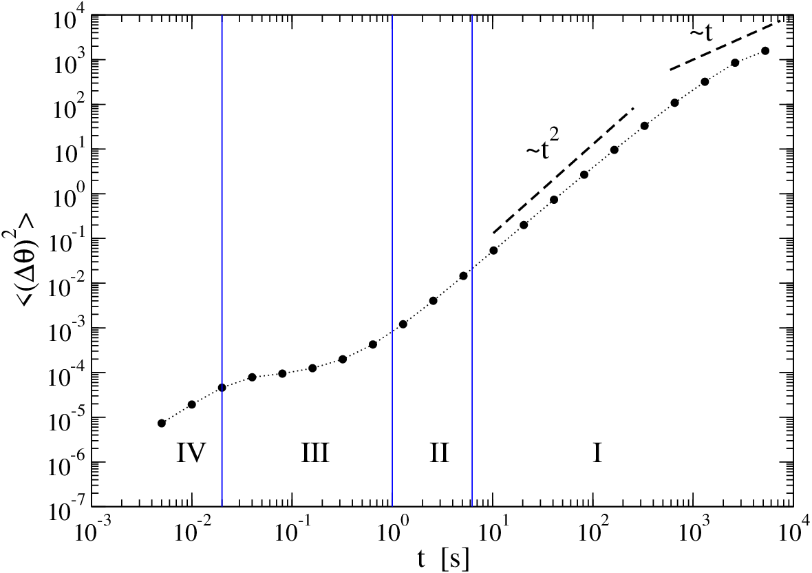
Mean-square-displacement (msd). The several phenomena observed in are reflected in the diffusion properties, see Fig. 3, where the mean-square displacement after a time is plotted. The four temporal regions corresponding to the frequency regions discussed above are marked on the graph. Our “cage-like” interpretation of the maximum of in region III is corroborated, in Fig. 3A, by the dramatic slowing-down of in the same region [24], resembling the typical dynamical slowdown in the diffusion of tracers dispersed in viscous liquids. At small times (region IV) the usual ballistic behavior appears. More remarkable is the behavior at large times. All the experiments with present a superdiffusive range in region II, with . For the largest values of , this behavior changes to a diffusive behavior in region I. On the contrary, at lower , the superdiffusive exponent remains the same of region II at large times. In particular, for , we find an almost ballistic superdiffusion . The situation is very different when the density is reduced (Fig. 3B): the long time behavior (region I) is always of the normal type . In the most dilute cases () the typical scenario of diffusion in a gas-like fluid is fully recovered in the form of a monotonic crossover from the ballistic region IV to the normal diffusion of region II and I. Changing the size and shape of the blade, see [21], does not lead to relevant changes in the above scenario.
The study of vpds and msd are consistent with measurements of the velocity-autocorrelation function (vacf) , which is the inverse Fourier transform of . In the very dilute cases, it is close to a simple exponential decay. The most dense and “cold” experiments, on the contrary, reveal a vacf with many features: a fast, though non-exponential, decay at small times, followed by a back-scattering oscillation through negative values, interpreted as the “cage”, and finally a slow decay to zero [25]. The final decay of the vacf could also light up the origin of superdiffusion. Unfortunately at large times the vacf is exceedingly noisy. A more promising way to probe long memory effects is to measure the times of persistency, i.e. the times during which the signal remains positively correlated. Our operative definition consists in two basic steps: 1) filter out high frequency oscillations which are not relevant for the behavior at large times of , by taking the running average over a large time ; and then 2) compute the statistics of the times separating two consecutive zeros of , which we call inversion time , see Fig. 4A and 4B for experimental samples of , and . The statistics of is a natural measurement of long term memory of the signal. The experimental probability density (pdf) of is shown in Fig. 4C- 4F for a few choices of parameters and values of . We observe that it rapidly decays with an exponential cut-off smaller or equal than in all cases where the msd asymptotically showed normal diffusion, signaling a finite memory of the dynamics. The cut-off apparently jumps to a much larger value in the cases where the msd displays superdiffusion: in such cases, the pdf decays to zero as a power or even slower. This is a fair evidence that long memory effects arise together with the observed superdiffusion. Long memory may be due to a slow rotating creeping motion of the surrounding granular medium, which acts as a coherent block and drags the blade. Such a “secondary” motion has long relaxation times due to the involved large inertia. New experiments are being designed with the aim of demonstrating this picture. We mention that longer experiments (shown in the SM [21]) still display superdiffusion that evolves in normal diffusion after many hours.


Modelling the dynamics of the blade. In the most dense and cold experiments, the vpds and the msd display an intriguing superposition of phenomena over almost decades of time-scales. It seems hopeless to reduce such a complexity to a model with a simple physical interpretation. It is tempting to disentangle the two main phenomena, i.e. caging (occurring at times smaller than ) and superdiffusion (more evident at times larger than ), by decomposing the dynamics into a slow and a fast component , with defined above. Experimental data demonstrate that the standard deviation of is much larger than that of and therefore dominates at short times (large frequencies). At long times (small frequencies), on the contrary, the fast dynamics averages out and emerges as the leading signal. For the fast dynamics, we propose a simple interpretation of the transient caging phenomena through a “diffusing harmonic cage” (dhc) model: this is a simplified version of the Itinerant Oscillator model describing translational and rotational diffusion of particles in liquids [26, 27], and reads
| (1a) | ||||
| (1b) | ||||
where and are white normal Gaussian noises. The model represents the diffusion of a particle in a harmonic potential with “stiffness” and unfixed minimum, under the effect of a thermal bath at temperature and relaxation time . The harmonic potential, representing the cage due to the confining effect of the dense granular host fluid, is not fixed but moves, as behaves as Brownian motion with diffusivity . Motivation for this model is twofold: 1) the main features of the vpds, i.e. an elastic resonance (region III) and a plateau revealing loss of memory at larger times (region II); 2) in the dilute limit it can be rigorously derived [28], while at intermediate densities a series of studies showed that memory effects (coming from correlated collisions) are well described by a coupling with an additional degree of freedom fluctuating at slower time-scales [23]. The vpds of the above model can be calculated and reads
| (2) |
Two limiting cases are recovered: when , the Ornstein-Uhlenbeck process is obtained, with taking the Lorentzian form mentioned before. When and , one has the Klein-Kramers process in a fixed harmonic potential, and for , expressing the absence of diffusion at large times: the cage does not move and fully confines the particle. Formula (2) fairly fits all experimental spectra in regions II and III, with parameters given in Tables 2 and 3 of [21]. Reasonably, the “cage stiffness” decreases at increasing shaking intensity. It also decreases as the density is reduced, and abruptly goes to zero for . The “cage diffusivity” rapidly increases with increasing and with decreasing . A more detailed study of the transition from the cage behavior to the free behavior is postponed to future investigations.
A more ambitious task is to devise a simple mechanism for , leading to superdiffusion. In driven granular systems it has been observed below the jamming transition [12] and in a few cases above it, where it was imputed to “zero”-modes of the host fluid [10], to Taylor dispersion [13], or to turbulence-like cascade effects [29]. We stress that, at variance with standard diffusion, for anomalous diffusion there is nothing similar to universality [30]. A systematic derivation of anomalous diffusion is a hard task and it is possible only in few specific cases [30]. Of course, the basic ingredient must be an enduring memory: a way to achieve it is to replace standard time derivatives with fractional derivatives in the Fokker-Planck equations, an approach which is subject of a vast literature [31]. Such an approach is capable, in principle, of describing both caging and superdiffusion within a single model equation, at the price of losing immediate interpretation and plain calculations. In a complementary approach [32] a coarse-grained value of (where only the sign of this quantity is traced) follows a continuous time random walk (ctrw): It takes discrete values with random transition times extracted from a given distribution. A simplified version of the ctrw is discussed in the SM [21]. We highlight that the ctrw gets a suggestive experimental confirmation in the observations of Fig. 4: indeed the ctrw model quantitatively connects the observed slow decay of to superdiffusion.
Conclusion: an experimental study of dense granular mesorheology allows to probe time-scales in a range of six orders of magnitude. Such an investigation reveals a complex scenario with different dynamical behaviors in four frequency or time regions. Three crucial features are observed at large density and low temperature: a “resonant” caging phenomenon at intermediate scales, non-white noise at fast scales, and super-diffusion at long times. The caging phenomenon is compatible with a diffusing harmonic cage model, while superdiffusion seems to be rooted in the long inversion times appearing in the dynamics , possibly related to creeping rotating motion of the granular media. A more detailed investigation of transitions is in order: a gas-liquid transition could be put in evidence by studying how when decreases; a liquid-glass transition could be taking place at the lowest values of or, eventually increasing . Superdiffusion and large values of could be signaling such a transition. Another promising line of investigation is active mesorheology, i.e. probing the response of the system to the application of an external force, achieved by coupling a controllable motor to the blade [19].
Acknowledgements.
We wish to thank A. Lasanta Becerra and A. Sarracino for useful discussions. AP acknowledges the support of the Italian MIUR grants FIRB-IDEAS n. RBID08Z9JE.References
- [1] B. Andreotti, Y. Forterre and O. Pouliquen, Granular Media. Between Fluid and Solid., Cambridge University Press (2013).
- [2] R. A. Bagnold, Proc. Royal Soc. London 225, 49 (1954).
- [3] G. H. Wortel, J. A. Dijksman, and M. van Hecke, Phys. Rev. E 89, 012202 (2014).
- [4] P. Wang, C. Song and H. A. Makse, Nat. Phys. 2, 526 (2006).
- [5] C. Song, P. Wang and H. A. Makse, Proc. Nat. Acad. Sci 102, 2299 (2005).
- [6] M. van Hecke, J. Phys.: Condens. Matter 22, 033101 (2010).
- [7] G. D’Anna, P. Mayor, A. Barrat, V. Loreto and F. Nori, Nature 424, 909 (2003).
- [8] N. V. Brilliantov and T. Pöschel, Kinetic Theory of Granular Gases, Oxford University Press (2004).
- [9] J. C. Dyre, Rev. Mod. Phys. 78, 953 (2006).
- [10] C. Heussinger, L. Berthier and J.-L. Barrat, Europhys. Lett. 90, 20005 (2010).
- [11] L. Cipelletti, S. Manley, R. C. Ball, and D. A. Weitz, Phys. Rev. Lett. 84, 2275 (2000).
- [12] F. Lechenault, O. Dauchot, G. Biroli and J. P. Bouchaud, Europhys. Lett. 83, 46003 (2008).
- [13] B. Utter and R. P. Behringer, Phys. Rev. E 69, 031308 (2004).
- [14] D. M. Mueth, G. F. Debregeas, G. S. Karczmar, P. J. Eng, S. R. Nagel and H. M. Jaeger, Nature 406, 385 (2000).
- [15] J. Brujić, C. Song, P. Wang, C. Briscoe, G. Marty, and H. A. Makse, Phys. Rev. Lett. 98, 248001 (2007).
- [16] T. M. Squires and T. G. Mason, Annu. Rev. Fluid. Mech. 42, 413 (2010).
- [17] G. Marty and O. Dauchot, Phys. Rev. Lett. 94, 015701 (2005).
- [18] A. L. Sellerio, D. Mari, G. Gremaud, and G. D’Anna, Phys. Rev. E 83, 021301 (2011).
- [19] A. Gnoli, A. Puglisi, A. Sarracino and A. Vulpiani, Plos One 9, e93720 (2014).
- [20] A. Naert, Europhys. Lett. 97 20010 (2012).
- [21] See Supplemental Material at [URL will be inserted by publisher] for details on experimental setup, theory and simulations.
- [22] M. B. Weissman, Rev. Mod. Phys. 60, 537 (1988).
- [23] A. Sarracino, D. Villamaina, G. Gradenigo, A. Puglisi, Europhys. Lett. 92, 34001 (2010).
- [24] P. M. Reis, R. A. Ingale, and M. D. Shattuck, Phys. Rev. Lett. 98, 188301 (2007).
- [25] A. Fiege, T. Aspelmeier, and A. Zippelius, Phys. Rev. Lett. 102, 098001 (2009).
- [26] V. F. Sears, Proc. Phys. Soc. 86, 953 (1965).
- [27] W. Coffey, Yu. P. Kalmykov and J. T. Waldron, The Langevin Equation: With Applications in Physics, Chemistry, and Electrical Engineering, World Scientific (Singapore, 1996)
- [28] A. Sarracino, D. Villamaina, G. Costantini and A. Puglisi, J. Stat. Mech. P04013 (2010).
- [29] F. Radjai and S. Roux, Phys. Rev. Lett. 89, 064302 (2002).
- [30] R. Klages, G. Radons and I. M. Sokolov (eds.), Anomalous transport, Wiley&Sons (2008).
- [31] J.Klafter, S. C. Lim and R. Metzler (eds.), Fractional Dynamics: Recent Advances, World Scientific (Singapore, 2012).
- [32] K.H. Andersen, P. Castiglione, A. Mazzino and A. Vulpiani, Eur. Phys. J. B 18, 447 (2000).
SM: SUPPLEMENTAL MATERIAL
I Details of the experimental setup
The scheme of our experimental setup is shown in Fig. 1A. A Poly(methyl methacrylate) (PMMA) container (diameter 90 mm, maximum height 47 mm and total volume 245 cm3) with an inverse-conical-shaped base, is filled with steel spheres (diameter 4 mm) and mounted on an electrodynamic shaker (LDS V450) which is fed, through an amplifier, with a noisy signal whose spectrum is approximately flat in a range with Hz and Hz. The shaker responds roughly linearly in the same range of frequencies, as verified with an accelerometer placed on the container. The elevation of the container at time is denoted by . We give the range of values for the relevant variables: for the maximum acceleration g, the maximum velocity mm/s and the maximum displacement mm. Details are reported below in Table 1. A PMMA blade (dimensions mm, momentum of inertia gmm2), suspended to a mounting which is mechanically isolated from the container/shaker apparatus, is immersed into the granular medium and can rotate around a vertical axis placed at the center of the container. The angular velocity of the blade and its absolute (i.e. without the modulus operation) angle of rotation are measured by an angular encoder (AEDA-3300) at a time-resolution of kHz and angular resolution 40000 divisions per revolution. The granular medium is in a liquid state because of the vibration. The blade, under the effect of the interactions with the spheres, performs a motion qualitatively similar to an angular Brownian motion. It is important to remark that the blade can only rotate and therefore moves along the “free flow” direction, i.e. it only probes the fluctuations of granular modes parallel to the boundaries of the container. Moreover, the blade’s size is such that, in the dense cases, its rotation is only allowed by the rearrangement of a large number of surrounding particles. We have performed two families of experiments: experiments at high density () and different normalized (i.e. in units) shaking intensities , and experiments at high shaking intensity () and different densities . In Fig. 1B and C we have reported the values of the mean squared angular velocity of the blade in the different experiments.
| 39.8 | 35.2 | 30.6 | 26.8 | 23 | 19.5 | |
|---|---|---|---|---|---|---|
| 0.25-0.06 | 0.22-0.05 | 0.19-0.05 | 0.17-0.04 | 0.14-0.04 | 0.12-0.03 | |
| 310.4-155.2 | 274.5-137.3 | 238.6-119.3 | 209-105 | 179.4-89.7 | 152-76 |
II Fits of the experimental data: parameters
| 39.8 | 0.54 | 0.0042 | ||||
| 35.2 | 0.53 | 0.0035 | ||||
| 30.6 | 0.51 | 0.0024 | ||||
| 26.8 | 0.5 | 0.0018 | ||||
| 23 | 0.47 | 0.0011 | ||||
| 19.5 | 0.44 | 0.00079 |
| 2600 | 0.54 | 0.0042 | ||||
| 2000 | 0.52 | 0.0055 | ||||
| 1300 | 0.54 | 0.0074 | ||||
| 700 (gas) | 0 | 1.1 | 0.069 | |||
| 350 (gas) | 0 | 1.1 | 0.2 |
III Experiments with blades of different sizes
We have performed a number of experiments with different blades, changing the total scattering surface and its shape. The thickness of the blades being constant, as well as its material, the mass and momentum of inertia are also varied accordingly.
In Figure 5a we portray the four shapes used. Shape “A” is the one used in the rest of the paper. Panels b and c of Figure 5 represent the vpds and the msd respectively, with the four shapes, in the case with and , corresponding to packing fraction . It appears that the general features of the vpds and msd are conserved when the size and shape of the blade are changed. Higher or smaller energy is obviously observed, when the inertia is reduced (shapes C and D) or increased (shape B). Differences in the mechanical (spurious) resonance at Hz are due to some modifications of the mounting mechanism on which the blade is fixed, occurred between the old and the new experiments. In the msd of the larger balde (shape B) it is observed - at large times - a saturation of the mean squared displacement which we impute to border effects. Note also that at very large time the measurement of the msd is noisy and prone to errors.


IV Very long experiments
The finite size of the experiment suggests that all relaxation times, even if long, are finite: the displacement , therefore, is expected to reach asymptotically a normal diffusive behavior. We have performed a -hours-long experiment in order to check such a hypothesis. The mean squared displacement is shown in Fig. 6. Indeed, at large times the superdiffusive behavior shows a crossover toward normal diffusion, which is slowly approached after many hours.
V The continuous time random walk model
A possible mechanism for superdiffusion is the continuous time random walk model (ctrw) [32, 30]. In the ctrw the variable (here the velocity) performs a random walk taking discrete values : it remains constant for a random time and then jumps to a new value. The choice of the statistics (pdf) of is the main parameter of the model and determines the properties of the autocorrelation of the velocity and, therefore, of the mean squared displacement.
Here we consider in details a simplified version of the ctrw model, where the velocity can take only two values. Such a simplification does not change the substance of the demonstration, which can be easily generalised to models with many possible values. Note that a comparison between this model and the experimental results should be made only at long time scales (i.e. such that is well approximated by ) and in the spirit of a strong coarse-graining, as if a dramatic loss of resolution allows to measure only the sign of the velocity.
In the model, changes its value at times with and . In the interval between and , takes the value . The intervals , with , are random and independent with the following probability density function
| (3) |
where is a smooth function: its shape and the value of (assumed to be always finite) are not relevant for the long time behavior of the displacement. The cut-off may eventually be taken to (see below).
For the msd therefore we have
| (4) |
and the values being independent and with zero average, one may drop the last term obtaining
| (5) |
The presence of the cut-off allows us to write
| (6) |
and therefore one finally has
| (7) |
The dependence on the cut-off (at large values of ) of the moments of order of are determined by the distribution at times larger than , i.e.
| (8) |
The last equality, together with Eq. (7), gives three possible behaviors for the msd at large times :
- •
for : normal diffusion, independently of the cut-off ;
- •
for : ;
- •
for : .
For , in the range , one expects . The value of can be determined by asking that it matches, at , the asymptotic behavior given above: for instance in the case the behaviors and can match only if ; the same argument for gives . The situation is therefore summarized here
| (9) |
Fig. 4 of the Letter shows that has an exponential cut-off at seconds for all the experiments where diffusive behavior is observed, that is in the most dilute or energetic cases. The cut-off rapidly grows and reaches times of the order of the duration of the experiment when and : a power law tail with emerges. Equation (9) makes this power law decay fully consistent with the ballistic behavior observed in Fig. 3 of the Letter.