Hierarchy problem, gauge coupling unification at the Planck scale, and vacuum stability
Abstract
To solve the hierarchy problem of the Higgs mass, it may be suggested that there are no an intermediate scale up to the Planck scale except for the TeV scale. For this motivation, we investigate possibilities of gauge coupling unification (GCU) at the Planck scale () by adding extra particles with the TeV scale mass into the standard model. We find that the GCU at the Planck scale can be realized by extra particles including some relevant scalars, while it cannot be realized only by extra fermions with the same masses. On the other hand, when extra fermions have different masses, the GCU can be realized around . By this extension, the vacuum can become stable up to the Planck scale.
I Introduction
The standard model (SM) like Higgs boson has discovered at the LHC experiment, and its mass is obtained by the ATLAS and CMS combined experiments as [1]. In the SM, this value of the Higgs mass leads the vacuum to be unstable, that is, the Higgs quartic coupling becomes zero below, but close to, the Planck scale ( GeV) [2]. The vacuum stability problem may suggest appearance of new physics below the Planck scale. If new particles appear beyond the SM, runnings of the gauge couplings become larger compared to the SM case. Then, the vacuum can be stable up to the Planck scale, since runnings of also becomes larger. Furthermore, the change of the running gauge couplings can realize the gauge coupling unification (GCU) at a high energy scale (see Ref. [3] for a general discussion).
In addition to the vacuum instability, the hierarchy problem of the Higgs mass would be appeared in the SM. In fact, the quadratic divergence of the Higgs mass term can be always multiplicatively subtracted at some energy scale from the Bardeen’s argument [4]. Since a renormalization group equation (RGE) of the Higgs mass term is proportional to itself in the SM, once it is zero at a high energy scale, e.g., the Planck scale, it continues to be zero at lower energy scales. However, if there are heavy particles coupling with the Higgs doublet, the Higgs mass term gives logarithmic correction as , where and are mass of the heavy particle and renormalization scale, respectively. Therefore, the hierarchy problem can be solved if no large intermediate scales exist between the electroweak and the Planck scales.
In this paper, we will consider that the Planck scale as a fundamental scale, in which the quadratic divergences are assumed to be completely removed out. To solve the hierarchy problem, we do not consider any intermediate scale except for the TeV scale. Under this context, we will investigate possibilities for the realization of the GCU at the Planck scale, and discuss the vacuum stability. This paper is based on our previous work [5].
II Requirement for the GCU
We investigate possibilities for the realization of GCU at some high energy scales. Solving the RGEs, we can see the behavior of the gauge couplings in an arbitrary high energy scale. The one-loop level RGEs of the gauge couplings are given by , where , 2, and 3, and the coefficients of , , and gauge couplings are given by (, , )=(41/6, , ) in the SM. For simplicity, we only consider a GUT normalization factor of 3/5 as in GUT, i.e. . Once particle contents in the model are fixed, contributions to are systematically calculated as in Table 1 [6]. In this table, fermions included vector-like to avoid the gauge anomalies.
| Irreducible representation | Contribution to (, , ) |
| (, , ) | by fermions |
| (1, 1, 0) | (0, 0, 0) |
| (1, 1, )(1, 1, ) | (, 0, 0) |
| (1, 2, )(1, 2, ) | (, , 0) |
| (1, 3, 0) | (0, , 0) |
| (1, 3, )(1, 3, ) | (, , 0) |
| (3, 1, )(, 1, ) | (, 0, ) |
| (3, 2, )(, 2, ) | (, 2, ) |
| (3, 3, )(, 3, ) | (, 8, 2) |
| (6, 1, )(, 1, ) | (, 0, ) |
| (6, 2, )(, 2, ) | (, 4, ) |
| (6, 3, )(, 3, ) | (, 16, 10) |
| (8, 1, 0) | (0, 0, 2) |
| (8, 1, )(8 1, ) | (, 0, 4) |
| (8, 2, )(8, 2, ) | (, , 8) |
| (8, 3, 0) | (, , 6) |
| (8, 3, )(8, 3, ) | (, , 12) |
| Irreducible representation | Contribution to (, , ) |
|---|---|
| (, , ) | by scalar particles |
| (1, 1, ) | (, 0, 0) |
| (1, 2, ) | (, , 0) |
| (1, 3, ) | (, , 0) |
| (3, 1, ) | (, 0, ) |
| (3, 2, ) | (, , ) |
| (3, 3, ) | (, 2, ) |
| (6, 1, ) | (, 0, ) |
| (6, 2, ) | (, 1, ) |
| (6, 3, ) | (, 4, ) |
| (8, 1, ) | (, 0, 1) |
| (8, 2, ) | (, , 2) |
| (8, 3, ) | (, , 3) |
To realize the GCU, we will consider extra particles with the TeV scale mass, which is motivated by avoiding the gauge hierarchy problem. Using the solution of the one-loop RGEs, one can obtain the GCU conditions as
| (1) |
where and are the mass scale of extra particles and the GCU scale, respectively. And, are contributions of the extra particles as . From Table 1, one can see and 1/6 for fermions and scalars, respectively. Figure 1 shows relations between and for fixed .

We can see that does not strongly depend on once a value of is fixed. It is worth noting that only or 1/2 can realize the GCU at the Planck scale, which are represented by two horizontal grid lines.11 1 If, however, we use two-loop RGEs and one-loop threshold corrections, values of gauge couplings in a high energy scale could have uncertainty. Thus, the GCU could be realized at the Planck scale even for and 2/3. Thus, one can find that, when all extra particles are fermions, the GCU at the Planck scale cannot be realized. This is the same result in Ref. [3]. On the other hand, when extra particles include some relevant scalars such as (1, 2, ), the GCU can be realized at the Planck scale as follows. For , the GCU can be realized at by extra particles satisfying
| (2) |
where the minimum value of is determined to satisfy , and the largest value of is determined to avoid the Landau pole. In the same way, for , the GCU can be realized at by extra particles satisfying
| (3) |
III Realization of the GCU at the Planck scale
According to the above discussions, we systematically investigate possibilities of the realization of GCU at the Planck scale, and find that a number of combinations of extra particles satisfy Eq. (2) or (3). For example, when we consider extra scalars are two doublets (1, 2, 0), the GCU can be realized around by extra fermions shown in Table 2. For simplicity, representation of extra fermions are the same as the SM fermions (with vector-like partners) and an adjoint fermion denoted by .22 2 Stable TeV-scale particles with fractional electric charge (such as the doublet scalar (1, 2, 0)) might cause cosmological problems. In order to avoid the problems, the reheating temperature after the inflation should be about 40 times lower than the particle masses [7], that is, in our cases.
| Extra fermions | (, , ) | ||
|---|---|---|---|
| (, , 4) | 28.0 | 7 | |
| (, 4, ) | 24.3 | 11 | |
| (, 4, ) | 24.3 | 11 | |
| (, , ) | 20.5 | 15 | |
| (, , ) | 20.5 | 15 | |
| (, , 6) | 16.8 | 19 | |
| (, 6, ) | 13.1 | 23 | |
| (, 6, ) | 13.1 | 23 |
Next, we consider extra fermions having different masses, which are taken as . Actually, we take only lepton masses 0.5 TeV, since lower bounds of vector-like lepton and quark masses are around 200 GeV and 800 GeV, respectively [8, 9, 10]. In Table 3, we show extra fermions which realize the GCU around . In the table, ” (0.5)” shows one (1, 3, 0) fermions with a mass of 0.5 TeV, and so on.
| Extra fermions | (, , ) | |
|---|---|---|
| (0.5) (1) (10) (10) | (, , 6) | 19.1 |
| (0.5) (2) (10) (10) | (, 6, ) | 14.9 |
| (0.5) (0.5) (1) (1) (10) (10) | (, , ) | 11.1 |
| (0.5) (0.5) (4) (10) (10) | (, , 8) | 7.95 |

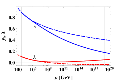
In Fig. 2 we show runnings of the gauge, the top Yukawa, and the Higgs quartic couplings, which correspond to the first one of Table 3. Here, we assume extra fermions do not strongly couple with the Higgs doublet, and then significantly change runnings of the top Yukawa and the Higgs quartic couplings. Since -functions of the gauge couplings change several times, our previous naive analyses are modified, that the GCU can be realized around by extra fermions satisfying . To realize the GCU, all the gauge couplings are large compared to those in the SM, which lead the smaller . Then, becomes larger and remains in positive value up to the Planck scale, since both the smaller and the larger make become larger. Thus, when the GCU is realized at the Planck scale, we expect the vacuum can become stable.
IV Summary
We have investigated possibilities of the GCU at the Planck scale in the extended SM which includes extra particles around the TeV scale. We have found that the GCU at the Planck scale can be realized when extra particles include some relevant scalars, while it cannot be realized (up to one-loop level) when all extra particles are fermions and their masses are the same. On the other hand, when extra fermions have different masses, the GCU around can be realized. In this case, the vacuum can become stable because of the change of the running gauge couplings.
Acknowledgements.
We thank N. Haba, R. Takahashi and H. Ishida for useful discussion and fruitful collaborations. The works of Y.Y. is supported by Research Fellowships of the Japan Society for the Promotion of Science for Young Scientists, Grants No. 262428.References
- [1] G. Aad et al. [ATLAS and CMS Collaborations], arXiv:1503.07589 [hep-ex].
- [2] D. Buttazzo, G. Degrassi, P. P. Giardino, G. F. Giudice, F. Sala, A. Salvio and A. Strumia, JHEP 1312, 089 (2013) [arXiv:1307.3536].
- [3] G. F. Giudice and A. Romanino, Nucl. Phys. B 699, 65 (2004) [Erratum-ibid. B 706, 65 (2005)] [hep-ph/0406088].
- [4] W. A. Bardeen, FERMILAB-CONF-95-391-T, C95-08-27.3.
- [5] N. Haba, H. Ishida, R. Takahashi and Y. Yamaguchi, arXiv:1412.8230 [hep-ph].
- [6] D. R. T. Jones, Phys. Rev. D 25, 581 (1982).
- [7] D. J. H. Chung, E. W. Kolb and A. Riotto, Phys. Rev. D 60, 063504 (1999) [hep-ph/9809453].
- [8] S. Chatrchyan et al. [CMS Collaboration], Phys. Lett. B 718, 348 (2012) [arXiv:1210.1797 [hep-ex]].
- [9] S. Chatrchyan et al. [CMS Collaboration], Phys. Lett. B 729, 149 (2014) [arXiv:1311.7667 [hep-ex]].
- [10] G. Aad et al. [ATLAS Collaboration], JHEP 11, 104 (2014) [arXiv:1409.5500 [hep-ex]].