An analysis of transient impulsive noise in a Poisson field of interferers for wireless channel in substation environments

Stochastic geometry approach is used to derive the first order of the characteristic function of interfering sources in presence of impulsive noise. Mathematical notations are inspired by [24]. First, we need to define the statistics of the interference field. Let $\Pi(\mathbf{r},t)$ be a random space-time field as a linear superposition of individual fields randomly produced by activated sources (emission of radiations) in a domain of sources. We postulate the Poisson random field $\Pi(\mathbf{r},t)=\sum_{i}\delta_{\mathbf{r}_{i},t_{i}}$ where $\delta_{\mathbf{r},t}$ is the Dirac measure on a finite space-time domain $\Lambda\subset\mathcal{R}^{3}\times\mathcal{R}$ where the three dimensional space is considered. We note that $\boldsymbol{\Psi}=\left\{\mathbf{r},t\right\}_{i}$ is a set of points representing active sources in the space-time domain $\Lambda$. Thus, the interference field can be written as :

where $\boldsymbol{\Upsilon}\in\mathcal{L}^{2}(\Omega,\mathcal{F},P)$ is an ensemble of measurable random waveforms of emitting sources, $d(\mathbf{r},\mathbf{r}_{0})$ is a distance parameter where $\mathbf{r}_{0}$ is the position of the antenna and $t|d(\mathbf{r},\mathbf{r}_{0})$ is related to the delay of propagation induced by the position of an interference source and the receiver. We now assume that these impulsive noise are separable functions such that the interference field can be written as :

where $N_{\mathbf{r}}$ is the point process related to emitting sources and $N_{t}$ is the point process of radiations in time domain. The intensity of measure of the point process $\mathcal{Z}\left(B\right)=E\left[\boldsymbol{\Psi}(B)\right]$, where $B$ is a Borel set, has a density $\lambda(\psi)=\lambda(\mathbf{r},t)$. By using Campbell’s theorem, the mean interference field is :

By assuming the ergodicity of the ensemble $\boldsymbol{\Upsilon}$ such that :

where $U_{\mathbf{r},t}$ is the basic waveform of interference sources. From the Laplace functional of the equation (3), the first order of characteristic function $Q(j\xi)$ of the superposition of these emitting radiations is given by :

The first order statistics such as moments, cumulants, amplitude distribution and density can be derived from the characteristic function which depends on the definition of the basic waveform of interference sources. It will be specified for impulsive interference sources in substation environments. The first order statistics of the interfering sources can be extended by considering an additive background noise.

In substation environments, radiations from interferers received at the antenna are impulsive and are caused by partial discharges mainly in air. They can be located in HV equipments when physical conditions are reached to discharge such as presence of defects, high electric field, free electrons etc, [25]. In presence of multiple interference sources in the vicinity of the antenna, a low density of space Poisson process $N_{\mathbf{r}}$ can be assumed where impulsive sources are randomly located in the three dimensional space in far-field region. For the activated impulsive sources, charge particles and currents produced by a discharge radiate impulsive electromagnetic radiations. The fields $\mathbf{E}$ and $\mathbf{B}$ can be obtained from retarded potentials $\mathbf{A}$ and $V$ respectively the magnetic potential vector and the scalar potential by :

The retarded vector and scalar potentials satisfying the Lorenz gauge condition can be written as a wave equation :

where $\rho(\mathbf{r},t)$ and $\mathbf{J}(\mathbf{r},t)$ are charge density and current density respectively of an activated sources $S_{i}$ on the emitting element $d\mathbf{v}^{{}^{\prime}}_{i}$ in $\mathbf{v}^{{}^{\prime}}_{i}$ as depicted on Fig. 1. The sum $\sum_{\mathbf{r}\in N_{\mathbf{r}}}$ represents the superposition of individual source randomly located in the vicinity of the antenna $R$. The speed of light in the medium is represented by $c$, $\varepsilon_{0}$ and $\mu_{0}$ are the permittivity and the permeability of the vacuum respectively. Each activated source $S_{i}$ radiates electromagnetic waves in the medium induced by retarded potentials. A receiver $R$ can received these waves on the receiving element $d\mathbf{v}_{R}$ in $\mathbf{v}_{R}$. By considering successive radiations from each source in the time domain, the Poisson process should be extended to space-time process.

Solution of equations in (7) is given by :

The interference sources are independent such that radiations at the antenna surface is a superposition of independent impulsive noise. Generally, the receiver has a directional radiation pattern not necessarily omnidirectional. The antenna has an effective length related to the induced voltage or current at the terminals to the incident field $\mathbf{E}$. The receiver may also have RF and IF (intermediate frequency) stages e.g, low noise amplifier and linear filters. As a result, the superposition of these radiations gives the typical waveform obtained from the receiver $R$ by :

where $a_{R}(\theta,\zeta,t)$ is the aperture weighting function in spherical coordinate system $(r,\theta,\zeta)$ respectively represented by the radial distance, the polar and the azimuthal angles. The aperture weighting function includes both the radiation pattern of the antenna and the linear impulse response of filters. It can be seen as an impulse response of the receiver where the receiving field is converted into a time waveform alone. The convolution product operates for temporal impulse response. The antenna receives the electric field $\mathbf{E}$, induced by the activated interferers, on the receiving element $d\mathbf{v}_{R}$ in $\mathbf{v}_{R}$. The resulting waveform $I_{t}$ is a superposition of independent impulsive noise $U_{t}$ produced by activated interference sources. The process $I_{t}$ is excited by a Poisson process $N_{t}$ related to the number of impulses in time domain. It is denoted as a shot-noise process [19, 26]. The typical impulsive noise $U_{t}$ after any RF and IF stages of (linear) filtering is written as :

where $\|u(\theta,\zeta)/r\|$ is the amplitude scale factor induced by geometry of interfering source and the receiver. $u(t)$ is the amplitude envelope and $\varphi(t)$ the instantaneous phase of the impulsive interference. In practice, receiving the signal at the receiver is distorted due to multipath propagation. Thus, the resulting impulsive noise is a random process where amplitude envelope and instantaneous phase are random processes. The propagation law may also induce the randomness of the amplitude scale factor. In addition, a background noiseshould be considered as combination of multiple independent interference sources below impulsive interference sources e.g, ambient noise from substations, thermal noise from receiver, etc.

We then fully write the random process $X_{t}$ as a combination of the shot-noise process $I_{t}$ with an additive background noise $n_{t}$ such that :

A common receiver design operates at a given carrier or center frequency. Therefore, the noise process has a resonant frequency such that impulsive noise is a transient signal with damped oscillation (see Fig. 2). It is seen that impulsive noise is distorted randomly due to constructive and destructive waves induced by the multipath channel related to the geometry of interference source and the receiver. It is argued that $U_{t}$ is generally non-stationary process where noise samples are non-i.i.d.

The receiver may have a local oscillator to recover any desired signals in baseband. In this condition, signals can be demodulated at the desired resonant frequency $\omega_{0}$. In complex domain, the baseband representation is given by :

where the instantaneous phase of any analytic signal is expressed as $\varphi(t)=\sum_{i}\omega_{i}t$ where the resonant frequency $\omega_{0}$ exist in $\varphi(t)$. Baseband signals may be more tractable for impulsive noise signal processing. Indeed, the power spectrum density can be estimated by using classical parametric spectral density estimation such as Yule-Walker method. As a result, these impulsive noise can be reproduced by using discrete-time series models such as autoregressive process.

Fig. 3 is an example of typical impulsive waveform and psd measured in a $735$ kV substation in baseband, demodulated at $f_{0}=800$ MHz. It is seen that a second order of AR process model gives suitable estimation of the decay of $\sim 1/f^{k}$ of the noise process. The non-i.i.d of noise samples in presence of an impulsive noise is induced by the decay of the power spectral density. The innovation process should be defined to compute distortions. The determination of first and second order statistics of the non-Gaussian process $X_{t}$ strongly depends on the specification of the impulsive shapes $U_{t}$, see the characteristic function in the equation (5). The basic waveform of the impulsive noise should take account physical parameters such as the duration of radiations, the non-stationary behaviour of the impulsive noise $U_{t}$ in which the amplitudes of the random process are non-i.i.d.

We consider real-valued random process $U_{t}$, the impulse shape received at the antenna produced by partial discharges as a discrete-time series such as an AR($p$) process model is given by :

where amplitude at the past samples $U_{t-i}$ are weighted by $\phi_{i}$ named AR($p$) coefficients. $\varepsilon_{t}$ is the innovation process that leads to distortions of $U_{t}$. We assume a second order of the AR($2$) process such that :

The AR coefficients $\phi_{1}$ and $\phi_{2}$ will be defined to ensure the stability of the process, i.e all its roots from the characteristic function lie outside the unit circle. Thus, the stationarity conditions should be verified. The second order of the AR process model allows to determined roots and the autocorrelation function of the random process $U_{t}$ easily.

The randomness of the process $U_{t}$ is induced by the innovation process $\varepsilon_{t}$. The latter should take account many random phenomena such as distortion of the impulsive shape and the non-stationary behaviour of the process linked by the duration of radiations received at the antenna. The definition of $\varepsilon_{t}$ is based on physical assumptions :

• •

  When an interference source is activated, radiations received at the antenna is a superposition of the constructive and destructive impulsive waves caused by multipath effects. These can be seen as a wave distorted by an i.i.d random variable $\varepsilon_{t}$ such that the equation (14) is satisfied.

• •

  Reflectors in substations cause multiple delayed paths that obey to the propagation law. In this condition, the amplitude of the impulse received at the antenna is necessarily decaying with respect to time until it vanishes below to the background noise i.e, $\varepsilon_{t}$ has a time-dependent parameter denoted by $\vartheta_{t}$ with the constraint that $\varepsilon_{t}$ is a function that decay over time or samples.

From these assumption, we can define $\varepsilon_{t}$ as a white noise where the variance is a discrete-time function, i.e, heteroscedastic white noise process [27, 28] :

where $\vartheta_{t}$ is the time-dependent standard deviation of the white noise process $W_{t}\sim\mathcal{N}(0,1)$. For those complex-valued random process $U_{t}$, one can consider complex-valued white noise process $W_{t}$. The discrete-time function $\vartheta_{t}$ can be defined as a positive power-law or log-normal function. The latter takes account rise time and a fall time of impulsive noise. Hence we write $\vartheta_{t}$ as :

where $\sigma_{t}$ is related to the time decay of the impulse. $\mu_{t}$ may refer to the time where the envelope of an impulse is maximum and may be related to the presence of the main path received at the antenna. $\vartheta_{0}$ is a normalized parameter. It is convenient that these parameters should be set such that the rise time and the decay time of an impulse are much shorter than the sample size of the non-Gaussian process.

A basic waveform of impulsive noise received at the antenna has been specified based on physical assumptions. The model produce impulsive noise waveforms where amplitude are distorted randomly by the innovation process as depicted on Fig. 4 where $dt$ is a time-increment defining a sample. The lined curve is the real-valued impulsive noise process where amplitudes should decay with respect to time represented by the dashed curve. The process is non-stationary due to the time-dependent of the standard deviation of the innovation process $\varepsilon_{t}$.

To ensure the stability of the process $U_{t}$, the stationarity conditions should be verified. By using the AR($2$) process model, we use the Box-Jenkins modelling approach [29]. The non-stationary process is differenced until stationary is achieved. Hence, from the equation (14), we write the difference-stationary process such that :

where $\Phi(L)=1-\phi_{1}L-\phi_{2}L^{2}$ and $L$ is the lag operator such that $U_{t}L^{i}=U_{t-i}$. Characteristic equation of the AR($2$) process is given by :

The quadratic equation (18) has two roots $r_{1}$ and $r_{1}$ where :

The roots depends on the value of the terms $\phi_{1}^{2}+4\phi_{2}$. The process has a stationary solution if and only if :

These AR coefficients specify the behaviour of the waveform of the impulsive noise $U_{t}$. They would help us to determine the problem statement for the determination of first and second order statistics of the non-Gaussian process $X_{t}$ in section IV.

By remembering that the innovation process is a heteroscedastic white noise process, the power spectral density of $U_{t}$ has a classical AR($2$) psd form given by :

where $S_{\varepsilon}(f)$ is the psd of $\varepsilon_{t}$. By using the equation (61) in Appendix A, we write the complete psd of $U_{t}$ as :

where $\sigma_{\vartheta}^{2}$ is the variance of $\vartheta_{t}$. The variance of the white noise is $\sigma_{W}^{2}=1$. Depending on the roots of the AR process, the psd of $U_{t}$ has different behaviour [30] :

• •

  For real roots, i.e, the terms $\phi_{1}^{2}+4\phi_{2}\geq 0$, if the characteristic equation has at least one real roots close to the unit circle, then $S_{U}(f)$ will have peak at $f=0$ if $\phi_{1}$ is positive. The psd will have peak at $f=0.5$ if $\phi_{1}$ is negative.

• •

  For complex roots, i.e, the terms $\phi_{1}^{2}+4\phi_{2}<0$, if the roots are closed to the unit circle, a peak occurs near the resonant frequency at $f_{0}$ given by :

  $$f_{0}=\frac{1}{2\pi}\cos^{-1}\left(\frac{\phi_{1}}{2\sqrt{-\phi_{2}}}\right)$$

  (23)

The impulse shape has a complex form due to the randomness of the amplitude. It may useful to provide the autocorrelation function (ACF) of the process $U_{t}$. From the roots of the characteristic equation on (18), the equation (17) is rewritten as :

where $G_{1}=1/r_{1}$ and $G_{2}=1/r_{2}$ remembering that $r_{1,2}$ are the roots of the quadratic equation (18). The autocorrelation denoted by $E\left[U_{t}U_{t-k}\right]\equiv\rho_{k}$ of the process $U_{t}$ following a closed form solutions :

The behaviour of the ACF $\rho_{k}$ depends on the nature of the roots of the quadratic function :

• •

  For real roots, with the constraint that $|G_{1}|$ and $|G_{2}|<1$, the ACF $\rho_{k}$ can be seen as mixture of damped exponentials or damped exponential oscillation that decay to zeros when $k$ increases.

• •

  For complex roots, the ACF is a damped sinusoidal function where the explicit expression of $\rho_{k}$ is given by [30] :

  $$\left(\sqrt{-\phi_{2}}\right)^{k}\frac{\sin\left(2\pi kf_{0}+\varsigma\right)}{\sin\left(\varsigma\right)}$$

  (26)

  where $f_{0}$ is the resonant frequency of the system and $\varsigma=(1-\phi_{2})/(1+\phi_{2})\cdot\tan(2\pi f_{0})$.

A general impulsive noise $U_{t}$ has been specified by using AR process model. If the stationarity condition of the process is ensured, one can reproduce a complete random waveform impulsive noise $U_{t}$ with damped oscillation at a desired resonant frequency by set the AR coefficient $\phi_{1}$ and $\phi_{2}$ such that the roots of the characteristic equation has complex roots. The impulsive noise can be represented in baseband where the psd $S_{U}(f)$ should have a peak at $f=0$. In this condition, the roots of the characteristic equation have to be real and particularly the first AR coefficient has to be positive, $\phi_{1}>0$.

We are now ready to derive the first and second order statistics of the non-Gaussian noise process $X_{t}$ based on the equation (5) by using the basic waveform $U_{t}$ of an impulsive interference from AR process model. However, it may be a non-trivial task since the impulsive noise shape has random amplitude. Some simplifying assumptions have to be considered. The second order statistics is the power spectrum of the process. It is given by the Carson’s theorem [23, 19].

We need to made some simplifying assumptions in terms of statistics from the basic Poisson field of interferers as well as in terms of basic waveforms of impulsive noise.

The description of the shape of amplitude distributions and densities can be given, in some extent, by moments and cumulants. For example, the skewness is a measure the asymmetry of noise and the kurtosis, a measure of how outlier-prone the distribution is. We start by calculating the $m^{\mbox{\small{th}}}$ cumulant $\kappa_{m}$ of the shot-noise process $I_{t}$. In equation (29), we assume $K$ as a random variable which assume positive and negative values make distributions. Then, from the extension of the Campbell’s theorem, the $m^{\mbox{\small{th}}}$ cumulant $\kappa_{m}$ is given by [19] :

where $Q_{I}(s)$ is the first order moment generating function of the shot-noise process. $\left\langle\cdot\right\rangle$ is the expectation taken over the distribution of the random variable. From binomial formula, we write the $m^{\mbox{\small{th}}}$ cumulant $\kappa_{m}$ as :

A series can be identified with a binomial sequence. By using the ratio test, we prove that $\kappa_{m}$ is convergent for infinite value of $m$ as seen in appendix B. Hence, $\kappa_{m}$ is necessarily finite. We extend to the non-Gaussian noise and by assuming the independence between the shot-noise process and the background Gaussian noise. Hence, we have :

Finally, for an additive background noise in which an i.i.d Gaussian noise of zero mean and variance $\sigma_{n}^{2}$ is assumed, $n_{t}\sim\mathcal{N}(0,\sigma_{n}^{2})$. Thus, we have :

We assume a non-negative impulsive shape such that $b$ higher than $a$. In this condition, for a finite value of $m=\{1,2,3,4,5,6\}$, the $m$-cumulants $\kappa_{m}$ is a non-monotonic sequence if $\left\langle K^{m}\right\rangle$ is negative for odd values of $m$, i.e $\kappa_{m}$ is negative for odd values and $\kappa_{m}$ is positive otherwise. The $m$-cumulants can be linked with the $m$-moments of the non-gaussian model. The skewness $\chi_{1}$ and the kurtosis $\chi_{2}$ are determined by the $3^{\mbox{\small{rd}}}$ and the $4^{\mbox{\small{th}}}$ standardized moments of the non-Gaussian noise $X_{t}$ respectively. They can be written in terms of cumulants such that :

• •

  The skewness value only depends on $\left\langle K^{3}\right\rangle$. Indeed, if the skewness is $|\chi_{1}|\leq 0$, then the probability density function of amplitude (pdf) can be left-skewed or right-skewed, i.e presence of longer tail on the left or on the right. The pdf can be also symmetric if $\left\langle K^{3}\right\rangle=0$. In practice, the asymmetry may be induced by random distortions of impulse shapes.

• •

  In presence of impulsive noise, if $\left\langle K^{4}\right\rangle>0$ and $\kappa_{4}>\kappa_{2}^{2}$, then the kurtosis is always $\chi_{2}>0$. Hence, the pdf can be leptokurtic, i.e a peak around the mean and long tail at higher amplitude values.

The moment generating function of the non-Gaussian noise is expressed by :

where $s\in\mathcal{R}$ and $Q_{I}(s)$ and $Q_{n}(s)$ are the moment generating function of the shot-noise $I_{t}$ and the additive background Gaussian noise $n_{t}$. The moment generating function of Gaussian noise $Q_{n}(s)$ is given by :

The generating function of the shot-noise process is more difficult to obtain. Nevertheless, a closed expression form of the moment generating function can be provided in terms of cumulant and by using the series expansion. We emphasize that the cumulant $\kappa_{m}$ is finite when $m$ goes to infinite as we proved in Appendix B. Hence, we start by the series expansion of the cumulant generating function of the shot-noise process such that :

Extended to the non-Gaussian noise, we link all values of the cumulant $\kappa_{m}$ as defined in equations (34) to the moments of the distribution. The cumulant generating function can be linked by the moment generating function $Q_{X}(s)$ where the cumulant generating function is the logarithm of the moment generating function :

where $\mu_{m}$ are moments of the distribution of the non-Gaussian noise such that :

The cumulant generating function can be seen as an entire function for complex values of $s$ where the function converges everywhere in the complex plane, (see Appendix B). Thus, the characteristic function $Q_{X}(j\xi)$ can be expressed by replacing $s=j\xi$ in the equation (39).

The power spectral density of the shot-noise process $I_{t}$ can be given in terms of the rate $\lambda$ and the Fourier transform of the impulse response of the associated linear filter by the Carson’s theorem [23, 19]. The power spectral density is given by the autocorrelation function of the non-Gaussian noise process $X_{t}$ is given by [19, 37, 20] :

The Carson’s theorem allow to express the power spectral density with these terms if the integral of the autocorrelation function of $\gamma_{t}$ is finite or equivalently, the integral of the psd is finite [19, 20]. We assume that $\left\langle K^{2}\right\rangle<\infty$. One can find the integral of psd of $\gamma_{t}$ is finite, $\int_{\mathcal{R}}S_{\gamma}(f)df<\infty~\forall f\in\mathcal{R}$. In this condition, extended to the non-Gaussian process, the resulting expression of the psd of $X_{t}$ is given by :

where $\omega=2\pi f$. It is seen that the psd of the non-Gaussian noise process has a decay of $\sim 1/f^{k}$.

In this section, the first and second order statistics can be derived from the basic waveform of the impulsive noise. We proved that we can have high value of kurtosis in which the distribution is leptokurtic and also be asymmetric as discussed. Furthermore, we proved that amplitude distributions and densities of the non-Gaussian process can be approximated by classical non-Gaussian pdf forms such as Middleton class A or $\alpha$-stable. The power spectral density can also be derived where a decay of $\sim 1/f^{k}$ is observed induced by waveforms of impulsive noise.

In section III, a complete random impulsive noise can be computed based on discrete-time series such as AR process. According to the equation (14), a second order of the AR process is used. We only restrict the discussion where impulsive noise are in baseband, i.e, a decay of $\sim 1/f^{k}$ with a peak at $f=0$. In this condition, we restrict AR coefficients such that their roots is real values and the stationarity condition is ensured, see equations (18) and (20c). The innovation process induced by $\varepsilon_{t}$ is a heteroscedastic white noise process where the time-dependent standard deviation is given by the equation (16). Parameters of the latter must be set such that the rise time and the decay time of a random impulsive waveform $U_{t}$ are much shorter than the sample size of the non-Gaussian process. Many random impulsive noise can be simulated as depicted on Fig. 5 where parameters are set as follows :

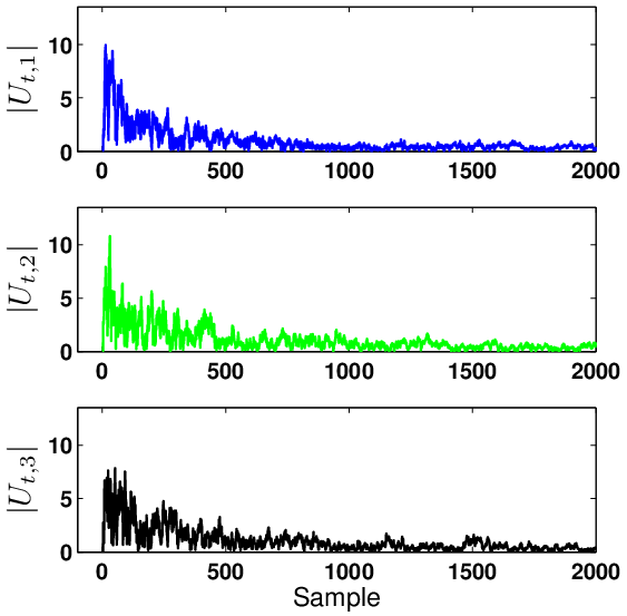
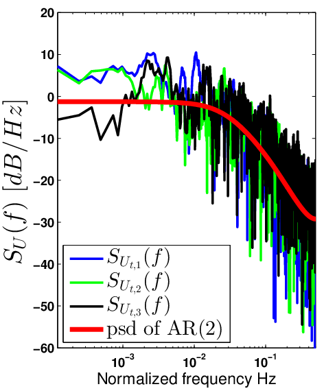
We see that the random process can generate many impulsive noise with random amplitudes but the power spectral densities have same behaviour, i.e a decay of $\sim 1/f^{k}$ closed to a Lorentzian form. The desired rise time and the decay time defining the duration of the impulse can be defined by setting parameters of the time-dependent standard deviation of the heteroscedastic process. One can be able to compute many random impulsive waveforms with many behaviours based on AR process as long as the stationarity condition is ensured.

Computer simulations and measurements are provided to validate the analysis.

References

- [1] E. J. Wegman, S. C. Schwartz, and J. B. Thomas, Topics in Non-Gaussian Signal Processing, S. N. York, Ed. Springer New York, 1989.
- [2] D. Middleton, “Non-gaussian noise models in signal processing for telecommunications : New methods and results for class A and class B noise models,” IEEE Transaction on Information Theory, vol. 45 no 4, pp. 1129–1149, 1999.
- [3] ——, “Statistical-physical models of electromagnetic interference,” IEEE Transactions on Electromagnetic Compatibility, vol. 19 Issue 3, pp. 106–127, 1977.
- [4] A. Spaulding and D. Middleton, “Optimum reception in an impulsive interference environment-part I: Coherent detection,” IEEE Transactions on Communications, vol. 25, pp. 910 – 923, 1977.
- [5] R. S. Blum, R. J. Kozick, and B. M. Sadler, “An adaptive spatial diversity receiver for non-gaussian interference and noise,” IEEE Transaction on Signal Processing, vol. 47 no 8, pp. 2100–2111, 1999.
- [6] G. Madi, B. Vrigneau, Y. Pousset, R. Vauzelle, and B. L. Agba, “Impulsive noise of partial discharge and its impact on a minimum distance-based precoder of MIMO system,” in 18th European Signal Processing Conference (EUSIPCO-2010), 2010, pp. 1602–1606.
- [7] G. Ndo, F. Labeau, and M. Kassouf, “A markov-middleton model for bursty impulsive noise : Modelling and receiver design,” IEEE Transactions on Power Delivery, vol. 28 no 4, pp. 2317–2325, 2013.
- [8] S. A. Bhatti, Q. Shan, I. A. Glover, R. Atkinson, I. E. Portugues, P. J. Moore, and R. Rutherford, “Impulsive noise modelling and prediction of its impact on the performance of WLAN receiver,” in 17th European Signal Processing Conference, 2009, pp. 1680–1684.
- [9] D. Middleton, “Man-made noise in urban environements and transportation system : Models and measurements,” IEEE Transactions on communications, vol. 21, no 11, pp. 1232–1241, 1973.
- [10] G. Tsihrintzis and C. Nikias, “Fast estimation of the parameters of alpha-stable impulsive interference,” IEEE Transactions on Signal Processing, vol. 44 Issue 6, pp. 1492–1503, 1996.
- [11] J. Chambers, C. Mallows, and B. Stuck, “A method for simulating stable random variables,” Journal of the American Statistical Association, vol. 71 no 354, pp. 340–344, 1976.
- [12] A. Weron and R. Weron, “Computer simulation of levy alpha-stable variables and processes,” Lecture Notes in Physics, vol. 457, pp. 379–392, 1995.
- [13] M. Zimmermann and K. Dostert, “Analysis and modeling of impulsive noise in broadband powerline communication,” IEEE Transactions on Electromagnetic Compatibility, vol. 44 no 1, pp. 249–258, 2002.
- [14] S. V. Vaseghi, Advanced Digital Signal Processing and Noise Reduction : Fourth Edition, J. W. . Sons, Ed. Wiley, 2008.
- [15] D. Middleton, Non-Gaussian Statistical Communication Theory, W.-I. Press, Ed. Wiley-IEEE Press, 2012.
- [16] X. Yang and A. Petropulu, “Co-channel interference modeling and analysis in a poisson field of interferers in wireless communications,” IEEE Transaction on Signal Processing, vol. 51 no 1, pp. 64–76, 2003.
- [17] K. Gulati, B. Evans, J. Andrews, and K. R. Tinsley, “Statistics of co-channel interference in a field of poisson and poisson-poisson clustered interferers,” IEEE transactions on Signal processing, vol. 58 no 12, pp. 6207–6222, 2010.
- [18] J. Llow and D. Hatzinakos, “Analytic alpha-stable noise modeling in a poisson field of interferers or scatterers,” IEEE transactions on Signal processing, vol. 46 no 6, pp. 1601–1611, 1998.
- [19] S. O. Rice, “Mathematical analysis of random noise,” Bell Syst. Tech. Journal, vol. 23, pp. 282–332, 1944.
- [20] S. B. Lowen and M. C. Teich, “Power-law shot noise,” IEEE Transactions on Information Theory, vol. 36 no 6, pp. 1302–1317, 1990.
- [21] ——, “Fractal shot noise,” Physical Review Letters, vol. 63 no 17, pp. 1755–1759, 1989.
- [22] D. Middleton, “Statistical-physical model of man-made radio noise, part I : First-order probability models of the instantaneous amplitude,” United States department of commerce office of telecommunications, Tech. Rep., 1974.
- [23] J. R. Carson, “The statistical energy-frequency spectrum of random disturbances,” Bell Syst. Tech. Journal, vol. 10 no 3, pp. 374–381, 1931.
- [24] F. Baccelli and B. Blaszczyszyn, Stochastic Geometry and Wireless Networks: Volume I Theory, N. Publishers, Ed. Now Publishers Inc, 2009.
- [25] R. Bartnikas and J. Novak, “On the character of different forms of PD and their related terminologies,” IEEE Transactions on Electrical Insulation, vol. 28, pp. 956–968, 1993.
- [26] E. N. Gilbert and H. O. Pollak, “Amplitude distribution of shot noise,” Bell Syst. Tech. Journal, vol. 39, pp. 333–350, 1960.
- [27] T. Bollerslev, “Generalized autoregressive conditional heteroscedasticity,” Journal of Econometrics, vol. 31, pp. 307–327, 1986.
- [28] R. F. Engle, “Autoregressive conditional heteroscedasticity with estimates of the variance of united kingdom inflation,” Journal of Econometrics, vol. 50 no 4, pp. 987–1007, 1982.
- [29] G. E. P. Box, G. M. Jenkins, and G. C. Reinsel, Time Series Analysis: Forecasting and Control 3rd ed., N. P. Hall, Ed. Englewood Cliffs, 1994.
- [30] W. A. Woodward, H. L. Gray, and A. C. Elliott, Applied Time Series Analysis, C. P. Taylor and F. Group, Eds. CRC Press Taylor and Francis Group, 2012.
- [31] J. E. Kolassa, Series Approximation Methods in Statistics, S. science + Business Media, Ed. Springer, 2006.
- [32] D. L. Wallace, “Asymptotic approximation to distribution,” Annals of Mathematical Statistics, vol. 29 no 3, pp. 635–654, 1958.
- [33] H. Daniels, “Tail probability approximations,” International statistical review, vol. 55 no 1, pp. 37–48, 1987.
- [34] R. Lugannani and S. O. Rice, “Saddle point approximation for the distribution of the sum of independent random variables,” Advances in Applied Probability, vol. 12 no 2, pp. 475–490, 1980.
- [35] G. Samarodnitsky and M. S. Taqqu, Stable non-Gaussian random processes : Stochastic models with infinite variance, C. P. LLC, Ed. CRC Press LLC, 2000.
- [36] B. V. Gnedenko and A. N. Kolmogorov, Limit distributions for sums of independent random variables, C. M. A.-W. P. Co., Ed. Cambridge Mass Addison-Wesley Pub Co., 1954.
- [37] S. O. Rice, “Mathematical analysis of random noise : part III,” Bell Syst. Tech. Journal, vol. 24, pp. 46–156, 1945.
- [38] R. J. V. Brunt, “Stochastic properties of partial-discharge phenomena,” IEEE Transactions on Electrical Insulation, vol. 26 no 5, pp. 902–947, 1991.
- [39] R. Schifani and R. Candela, “A new algorithm for mixed weibull analysis of partial discharge amplitude distributions,” IEEE Transactions on Dielectrics and Electrical Insulation, vol. 6 no 2, pp. 242–249, 1999.
- [40] M. Au, F. Gagnon, and B. L. Agba, “An experimental characterization of substation impulsive noise for a RF channel model,” Progress In Electromagnetics Research Symposium, PIERS Proceedings, vol. 1, pp. 1371–1376, 2013.
- [41] S. M. Zabin and H. V. Poor, “Efficient estimation of class A noise parameters via the EM [expectation-maximization] algorithms,” IEEE Transaction on Information Theory, vol. 37 no 1, pp. 60–72, 1991.
- [42] D. Middleton, “Procedures for determining the parameters of the first-order canonical models of class A and class B electromagnetic interference,” IEEE Transactions on Electromagnetic Compatibility, vol. 21 Issue 3, pp. 190–208, 1979.
- [43] I. A. Koutrouvelis, “Regression-type estimation of the parameters of stable laws,” Journal of the American Statistical Association, vol. 75 no 372, pp. 918–928, 1980.
- [44] ——, “An iterative procedure for the estimation of the parameters of stable laws,” Communications in Statistics-Simulation and Computation, vol. 10 no 1, pp. 17–28, 1981.
- [45] J. G. Proakis and D. G. Manolakis, Digital Signal Processing : Princples, Algorithms and Applications Fourth edition, P. P. Hall, Ed. Pearson Prentice Hall, 2007.
- [46] S. L. Marple, Digital spectral analysis with applications, P. P. Hall, Ed. Pearson Prentice Hall, 1987.