Index Coding and Network Coding via Rank Minimization
Abstract
Index codes reduce the number of bits broadcast by a wireless transmitter to a number of receivers with different demands and with side information. It is known that the problem of finding optimal linear index codes is NP-hard. We investigate the performance of different heuristics based on rank minimization and matrix completion methods, such as alternating projections and alternating minimization, for constructing linear index codes over the reals. As a summary of our results, the alternating projections method gives the best results in terms of minimizing the number of broadcast bits and convergence rate and leads to up to savings in average communication cost compared to graph coloring algorithms studied in the literature. Moreover, we describe how the proposed methods can be used to construct linear network codes for non-multicast networks. Our computer code is available online.
I Introduction
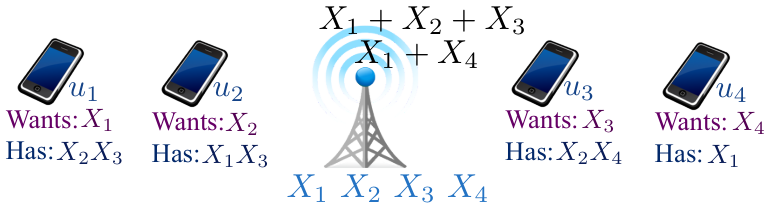
We investigate the performance of different rank minimization heuristics for constructing linear index codes [1, 2], and therefore linear network codes using the equivalence in [3, 4]. Index codes reduce the number of bits broadcast by a wireless transmitter that wishes to satisfy the different demands of a number of receivers with side information in their caches. Fig. 1 illustrates an index coding example. A wireless transmitter has packets, or messages, and there are users (receivers) . User wants packet and has a subset of the packets as side information. The packets in the cache could have been obtained in a number of ways: packets downloaded earlier, overheard packets or packets downloaded during off-peak network hours. Each user reports to the transmitter the indices of its requested and cached packets, hence the nomenclature index coding [5]. Assuming an error-free broadcast channel, the objective is to design a coding scheme at the transmitter, called index code, that satisfies the demands of all the users while minimizing the number of broadcast messages. For instance, the transmitter can always satisfy the demands of all the users by broadcasting all the four packets. However, it can save half of the broadcast rate by transmitting only coded packets, and to the users. Each user can decode its requested packet by using the broadcast packets and its side information. The problem that we focus on here is is how to construct linear index codes that minimize the number of broadcast messages.
Contribution
Answering the question above turns out to be an NP-hard problem in general [6, 7, 8]. Motivated by a connection between linear index codes and rank minimization [5] (details in Sec. III-B), we propose to use rank minimization and matrix completion methods to construct linear index codes. The underlying matrices representing an index coding problem have a special structure that affects the performance of these methods. For instance, the celebrated nuclear norm minimization method [9, 10] does not perform well here. We present our findings on the performance of different other methods, such as alternating projections, directional alternating projections and alternating minimization, through extensive simulation results on random instances of the index coding problem. These methods are performed over the real numbers and give linear index codes over the reals which have applications to topological interference management in wireless networks [11, 12]. As a sample of our results, Fig. 2 compares the performance of index codes obtained by the Alternating Projection (AP) method to other methods studied in the literature. We assumed that packets are cached independently and randomly with probability . The figure shows the savings in communication cost resulting from using index codes compared to no-coding and multicast network coding (all users decode all messages). The AP method leads to up to average savings in broadcast messages compared to graph coloring [1, 6].
Over the recent years, several connections have been established between index coding and other problems. These connections can be leveraged to apply the rank minimization methods presented here to these equivalent problems. For instance, using the reduction between index coding and network coding devised in [3, 4] to show the equivalence of the two problems, the methods proposed here could be readily applied to construct linear network codes over the reals [13, 14] for general non-multicast networks. Similarly, these methods can be used to construct certain class of locally repairable codes (over the reals) using the duality between index codes and locally repairable codes established in [15, 16]. Our computer code for constructing linear index codes, network codes and locally repairable codes is available online [17].
Related work
Index coding was introduced by Birk and Kol in [1] as a caching problem in satellite communications. The work of [5] established the connection between linear index codes and the minimum rank of the side information graph representing the problem. The sub-optimality of linear index codes was shown in [18, 19, 20]. The work of [21] further explored the connection to graph coloring and studied properties of index coding on the direct sums of graphs. Linear programming bounds were studied in [22] and connections to local graph coloring and multiple unicast networks were investigated in [23] and [16], respectively. The work in [24] investigated the property of index codes on random graphs. Tools from network information theory [25, 26] and distributed source coding [27] were also used to tackle the index coding problem. Related to index coding is the line of work on distributed caching in [28, 29]. Recently, a matrix completion method for constructing linear index codes over finite fields was proposed in [30], and a method for constructing quasi-linear vector network codes over the reals was described in [31].
Organization
The rest of the paper is organized as follows. In Section II, we describe the mathematical model of the index coding problem and the assumptions we make. In Section III, we summarize the connections of index coding to graph coloring, rank minimization and topological interference management. In Section IV, we focus on index coding instances that can be represented by undirected graphs. We describe the different rank minimization methods and our simulation results. In Section V, we describe the performance of these methods for directed graphs. In SectionVI, we elaborate more on the use of rank minimization methods for constructing linear network codes. We conclude in Section VII.
II Model
An instance of the index coding problem is defined as follows. A transmitter or server holds a set of messages or packets, , where the ’s belong to some alphabet. There are users, . Let (“wants” set) represents the packets requested by , and the set (“has” set) represents the packets available to as side information in its cache. WLOG, we can assume that contains only one packet, otherwise the user can be represented by multiple users satisfying this condition. We assume that initially the transmitter does not know which packets are cached at each user, and the users tell the transmitter the indices of the packets they have in an initial stage. Typically, the alphabet size (packet length) is much larger than the number of packets , so the overhead in the initial stage is negligible. The transmitter uses an error-free broadcast channel to transmit information to the terminals. The objective is to design a coding scheme at the transmitter, called index code, that satisfies the demands of all the users while minimizing the number of broadcast bits. We will focus on linear index codes in which the messages belong to a certain field ( or ) and the transmitted messages are linear combinations of these messages. Linear index codes are known not to be optimal [19] and the gap to optimality can be arbitrarily large [18]. However, we focus on linear codes due to their tractability. For clarity of exposition, we make the following two assumptions:
- 1.
The number of users is equal to the number of messages (). We will assume that user requests message , i.e., . It was shown in [32] that any general instance, , can be reduced to this model with no loss of generality for linear codes.
- 2.
The messages are atomic units that cannot be divided. This corresponds to scalar linear index codes. We refer to the number of broadcast messages as the index code length. We denote by the minimum number of broadcast messages achieved by scalar linear index codes. Our methods could be easily extended to vector linear index codes for a givenblock length.
III Connections to Other Problems
III-A Index Coding & Graph Coloring
The minimum scalar linear index codes length can be upper bounded by the chromatic number of a certain graph. An index coding problem, with messages and users11 1 In the case where there are more users than messages, i.e., , the index coding problem can be represented by a multigraph [21] or a bipartite graph [16]., can be represented by a directed graph , referred to as side information graph, defined on the vertex set . An edge is in the edge set of iff user has packet as side information.
The side information graph representing the instance in Fig. 1 is depicted in Fig. 3(a). Its maximal undirected subgraph in Fig. 3(b) is obtained from by replacing any two edges in opposite directions by an undirected edge, and removing the remaining directed edges. We will say that is undirected if and are the same graph. A fully connected subgraph (clique) of represents a subset of users that can be satisfied simultaneously by broadcasting a single coded packet that is the XOR of all the packets indexed by the clique. Therefore, a partition of into cliques gives a scalar linear index code over any field. We can optimize such a partition in order to obtain a minimum number of cliques. Such a number is called the minimum clique cover, , of (see Fig. 3(b)). Note that the minimum clique cover number is equal to the chromatic number of the complement graph (Fig. 3(c)), and therefore finding it is an NP-hard problem [33, 34]. Fig. 3(b) shows a minimum clique cover of and the resulting index code of rate , and therefore clique cover based index codes are not necessarily optimal. Nevertheless, it is the basis of many greedy heuristics in the literature [2, 6].
A lower bound on is the independence number which is the maximum number of vertices with no edge between any two of them. To see this, consider the sub-problem formed by the users corresponding to an independent set of and their messages. In this sub-problem, users do not have any side information and therefore all the messages must be transmitted. We summarize the results above in the following Lemma.
Lemma 1
.
III-B Index Coding & Rank Minimization
It was shown in [5] that finding an optimal scalar linear index code is equivalent to minimizing the rank of a certain matrix . For instance, this matrix for the example in Fig. 1 is given by
The matrix is constructed by setting all the diagonal elements to ’s, a star in the position if edge exists in , i.e., user caches packet , otherwise the entry is . The intuition is that the th row of represents the linear coefficients of the coded packet that user will use to decode . Hence, the zero entries enforce that this coded packet does not involve packets that does not have as side information. The packets that has as side information can always be subtracted out of the linear combination. The goal is to choose values for the stars “” from a certain field such that the rank of is minimized. The saving in transmitted messages can be achieved by making the transmitter only broadcast the coded packets that generate the row space of . It turns out that this formulation of index coding coincides with the minimum rank of a graph , , defined by Haemers [35]. Therefore, the optimal rate for a scalar linear index code is [5].
III-C Index Coding & Topological Interference Management
It was shown in [11] that, in the linear case, the index coding problem is equivalent to the topological interference management problem in wireless networks. The latter problem consists of finding optimal transmission schemes in interference networks with no channel state information at the transmitter. This equivalence holds over any field, in particular the field of real numbers on which we focus in this paper.
We will briefly describe this equivalence using an example and refer the interested reader to the results in [11] and related literature [12, 36] for more details. Fig. 4 depicts the wireless interference network that is equivalent to the index coding problem in Fig. 1. Black solid links connect a transmitter with its intended receiver . Dashed red links indicate the set of receivers with which a transmitter node interferes when transmitting. For example, transmitter interferes with receiver . Transmitted signals are added “in the air” and a receiver will receive the sum of his intended signal plus the interference on the red links. The intuition behind the connection to index coding can be explained as follows. Take for example receiver , it does not suffer of interference from and which is equivalent to getting interference from all the transmitters and possessing the messages of and as side information, so it can cancel them out. One communication scheme for this network consists of letting each transmitter sends his message during a different time slot while the other transmitters are “off”. This corresponds to the trivial index coding solution of sending all the messages. The index code in Fig. 1 gives a more efficient scheme for interference network in Fig. 4: nodes transmit together in the first time slot, then nodes transmit together in the second time slot.
IV Index Coding on Random Undirected Graphs
We start by considering undirected side information graphs (), i.e., for every directed edge in there is an edge in the opposite direction. Our approach is to use convex optimizing methods to find by minimizing the rank of the matrix over the reals. The problem of rank minimization has been extensively studied in system theory [37, 38]. In [10, 9], it was shown that the convex relaxation that replaces the rank function by the nuclear norm (sum of singular values) leads to finding the minimum rank with high probability under certain conditions on the matrix rank and the number of fixed (observed) entries in the matrix. However, these results do not carry over directly to the index coding problem because the model there assumes the location of the fixed entries is chosen uniformly at random. In contrast, the index coding matrix has a specific structure that dictates all the the diagonal entries to be equal to one. Indeed, the semi-definite program (SDP) relaxation in [9] always output the maximum rank (instead of the minimum rank) which is obtained by setting all the “*” entries in to zero making it the identity matrix (see Appendix A). Next, we will show that other rank minimization methods, such as the alternating projections (AP) method [38, 39], can be used to construct near-optimal scalar linear index codes.
IV-A Alternating Projection Method
Given two convex regions and , a sequence of alternating projections between these two regions converges to a point in their intersection as illustrated in Fig. 5(a) [40, 39, 38]. Therefore, completing the index coding matrix by choosing values for the “*” such that has a low rank can be thought of as finding the intersection of two regions and in , in which
| (1) |
is the set of matrices of rank less or equal to a given rank , and
| (2) |
Note that is not convex and therefore convergence of the AP method is not guaranteed. However, the AP method can give a certificate, which is the completed matrix , that a certain rank is achievable. Therefore, we will use the AP method as a heuristic as described in algorithm 1.
Algorithm 1: The projection of a matrix on the region is obtained by singular value decomposition (SVD) [41]. We noticed from our simulations that a considerable improvement in performance and convergence rate, (See Figs. 16 and 17 in Appendix F) can be obtained by projecting on , the set of positive semi-definite matrices of rank less or equal than ,
| (3) |
The projection on is obtained by eigenvalue decomposition and taking the eigenvectors corresponding to the largest eigenvalues, as done in Step 1. The Projection on region is obtained by setting the diagonal entries of the matrix to and the th entry to if edge does not exist in , as done in Step 1 and 1.
Theoretically, the time complexity of the algorithm can be reduced by doing a binary search on . However, we found that it is much faster to start with equal to the coloring number returned by the greedy coloring algorithm (Step 1). The stopping criteria in Step 1 uses the norm, , which is equal to the largest singular value of the matrix.
IV-B Simulation Results
We tested the performance of algorithm 1 on randomly generated graphs. We used the Erdos-Renyi model to generate random undirected graphs on vertices where edges between two vertices are chosen iid with probability . We compared the performance of algorithm 1 to greedy coloring22 2 We used the greedy coloring function in the mathgraph Matlab Library. and Least Difference Greedy (LDG) (see Appendix B for details on LDG). We also tested the Alternating Minimization method (AltMin) [38, 42, 43] described in Appendix C. It does not perform as good as AP (see Fig. 18) and suffers from a slow convergence rate.
Fig. 6 shows the average rank obtained by the APIndexCoding algorithm for between and and different values of . In all our simulations, each data point is obtained by running the algorithms on graph realizations and in the stopping criterion. The APIndexCoding algorithm always outperforms LDG and Greedy coloring. For instance, an improvement of over greedy coloring is obtained for and . Fig. 7 shows the histogram of the distribution of the rank by APIndexCoding which suggests a concentration around the mean of ranks returned by APIndexCoding33 3 The concentration of the minimum rank of around its average can be proven using the vertex exposition martingale method [44]. However, finding an expression of the average remains an open problem [24].. Fig. 8 shows the savings achieved by APIndexCoding over linear network codes which allow all users to decode all the messages (multicast)44 4 Linear network codes can achieve multicast by transmitting . Similarly, Figs. 19, 20 and 21 in Appendix F show the percentage savings of APIndexCoding over uncoded transmissions, greedy coloring and LDG.
Lower bounds: We tested the APIndexCoding algorithm on all non-homomorphic directed graphs on at most vertices and compared its performance to the optimal rates reported in [45]. APIndexCoding was always able to find the optimal index coding length except for when it is not an integer ( graphs on vertices). Moreover, we tested APIndexCoding on random 3-colorable graphs (3-partite graphs). For these graphs, we know a priori that the matrix could be completed to have rank or less. Fig. 9 shows that APIndexCoding beats greedy coloring and LDG and gives an average rank very close to .
IV-C Convergence Rate and Running Time
We ran the simulations on a DELL XPS i7 - 16GB Memory Desktop using Matlab software. Figs. 10 and 23 depict respectively the average time and average number of iterations taken by the APIndexCoding algorithm to converge on a random undirected graph . We notice that the time complexity of the algorithm roughly increases exponentially as increases (and constant) and as increases (and constant).
To speed up the converge time, we tested a variant of the AP method, called Directional Alternating Projections (DirAP) [46] which is described in Appendix D. DirAP can lead to considerable savings in time as seen in Fig. 11 ( for and for , both for ). We should mention that Greedy coloring and LDG have complexity quadratic in and are therefore much faster than Directional APIndexCoding as seen in Fig. 11. However, the savings in transmissions induced by DirAP or APIndexCoding may justify their computation overhead in scenarios where the computation can be done offline or can be amortized over a long time such as finding codes for interference networks with static or slowly changing topologies.
IV-D Decoding Error Analysis
The 1 algorithm returns a completed matrix with low rank . However, is not in in general, but is very “close” to a matrix in (in norm distance) as dictated by to the stopping criteria of the algorithm. This will cause a small decoding error at the users side.
Example 2
For the index coding instance of Fig. 1, our implementation of algorithm 1 with returns following matrix with rank ,
| (4) |
It can be seen that is not in since that the positions that are supposed to be zero are not exactly but relatively small numbers.
The next result shows that if the quantization interval of the messages ’s is not very small, the decoding error can be avoided. Assume , and let be the decoded message . Lemma 3 upper bounds the decoding error as a function of , where is the distance of the matrix to and is used as a stopping criteria in 1.
Lemma 3
Let be the message vector at the transmitter. Assume that the index code given by matrix is used and let be the messages decoded by the users. Then,
| (5) |
Proof:
See Appendix E. ∎
To illustrate the result in Lemma 3, we first elaborate on the encoding and decoding functions of the index code once is obtained from the algorithms.
Let be the rank of and Let be a submatrix of of rank . WLOG, we can assume that is formed of the first rows of . Let denotes the th row of , with .
The transmitter broadcasts
| (6) |
When decoding, user can obtain by the following decoding equation:
| (7) |
where is the Moore-Penrose pseudoinverse of and is a dimension vector that contains all the side information that user has, with ’s on all the other positions. For instance, in the example of Fig. 1,
Example 2 (continued): Suppose the transmitter wants to send to the users. Let
be a submatrix of in (4) of rank . Then, the transmitter should broadcast The decoding vector given by (7) is
The aggregate decoding error here is . This should be compared to the bound from Lemma 3 which gives
In general, it would be interesting to bound the decoding error per user. However, we found it more tractable to bound the aggregate decoding error. The bound on the decoding error in Lemma 3 is loose, but can give guidelines on how the stopping criteria affects the decoding error and can help design the quantization of the source if zero-decoding error is required. Fig. 12 shows the gap between the theoretical bound of Lemma 3 and the average error obtained in simulations.
V Index Coding on Random Directed Graphs
In this section, we consider the more general case in which the side information graph is a directed random graph. Each directed edge exists with probability and the graph edges are chosen independently. In this case, we can apply all the rank minimization methods described in the previous section on the graph , the maximal undirected subgraph of . In addition, we can apply the AP and Directional AP methods via SVD directly on the graph (SVD is needed here because the matrix is not symmetric). Fig. 13 depicts the top three among these methods having the best performance. For relatively small values of , DirSVDAP on the directed graph has the best performance. However, for large APIndexCoding on performs better. It is worth mentioning that this directed random graph model was used in Fig. 2 and the results on alternating projections there were also obtained by applying APIndexCoding algorithm on .
To address the practical setting in which users have a fixed cache size, we evaluated the performance of these methods on random directed regular graphs. These results are presented in Fig. 24 and show that APIndex coding gives the best results in terms of minimizing the index code length.
VI Network coding via Rank Minimization
Network coding can be thought as a generalization of routing schemes in networks. It allows intermediate nodes to forward coded packets that are functions of their incoming packets [47, 48, 49]. There are now efficient algorithms to construct capacity-achieving network codes for multicast networks and some related variants [50, 51, 52, 53]. However, making similar progress for general networks with non-multicast demands is believed to be a very hard problem [54, 55, 56, 57], even for two-unicast networks [58]. With this backdrop, the rank minimization heuristics presented here provide a computational tool that contribute to making progress towards constructing linear network codes for non-multicast networks.
The main idea here is to use the efficient reduction in [3, 4] to transform a given network coding problem to an index coding problem and then to apply the rank minimization methods presented here to . Suppose that is defined over a network with vertex set , edge set , and each edge has capacity . The reduction guarantees the following property: has a network code over a certain alphabet that allows all the destinations to decode their messages with zero probability of error if and only if has an index code of length over the same alphabet. This property gives the algorithm illustrated in Fig. 14. The proposed rank minimization methods are not guaranteed to find the minimum rank (i.e., minimum scalar linear index code length), but can give a certificate (the completed matrix) for the low rank it find. For this reason, the algorithm in Fig. 14 either outputs a linear network code solution or a “do not know” message. This algorithm was implemented in Matlab and can be found and tested on the link in [17].
VII Conclusion
We have investigated the performance of different rank minimization methods for constructing linear index codes over the reals. Our simulation results indicate that the Alternating Projections method and its directional variant, always outperform (smaller code length) graph coloring algorithms, and they converge much faster than the Alternating Minimization method. Due to the special structure of the underlying matrices representing the index coding problem (all ones diagonal), the well-studied nuclear norm minimization method performs badly here. Our results lead to the following open questions that we plan to address in our future work:
- 1.
Can the proposed methods here be adapted to construct linear index codes over finite fields?
- 2.
Under what conditions on the index coding matrices, can these methods be given theoretical guaranties to construct optimal linear index codes?
VIII Acknowldgement
The second author would like to thank Prof. Stephen Boyd for suggesting the use of the alternating projections method, Borja Peleato-Inarrea and Carlos Fernandez for discussions on the alternating minimization method and Alex Dimakis for insightful discussions on index coding and graph coloring.
Appendix A Nuclear norm minimization
Using the nuclear norm minimization method to minimize the rank of the index coding matrix will always give the maximum rank . This corresponds to the trivial index code obtained by replacing all the “*” in by zero. This follows directly from the results in [10] which we reproduce here for completion. Let denotes the nuclear norm.
Lemma 4
The nuclear norm can be written as,
where is the trace of a matrix.
In the previous lemma, if we pick to be the identity matrix then Therefore, applying the nuclear norm minimization to the index coding problem will always return the diagonal matrix as the optimal solution.
Appendix B LDG Algorithm:
Birk and Kol proposed a greedy algorithm named Least Difference Greedy (LDG) in [1, 2] for finding scalar linear index codes. LDG can be regarded as a heuristic for finding clique cover for graphs. The idea is to minimize the rank of the index coding matrix by greedily searching for rows that could be made equal and “merging” them. Two rows are mergeable if there does not exist any column in which one of these rows has a and the other a . Therefore, the two rows can be made the same by giving appropriate values to . For instance, in the example of Fig. 1, we start from matrix
Row and row are mergeable. After merging them we get
There are no more mergeable rows in . The remaining “*”’s can be set arbitrarily, for example they could be set all to . And, the LDG algorithm will output the transmitted messages , and . For completion, we give next the details of the LDG algorithm as proposed in [1, 2].
Appendix C Alternating Minimization Algorithm:
The Alternating Minimization (AltMin) is now a well studied method for rank minimization [38, 42, 43]. We briefly describe it here for completion.
If the matrix has rank then it can be factored as where and and is the transpose of . Thus, the problem becomes the following
| (8) |
where denotes the Frobenius norm. The optimization problem in (8) is not convex. However, it will become convex if either or is fixed. Algorithm 3 [38] shows the iterations between fixing and and solves the resulting convex problem at each time (Steps 5 and 6, respectively). Each of these steps is a least squares problem that has an analytical solution [59, p. 4-5].
Appendix D Directional Alternating Projections:
The Directional Alternating Projections (DirAP) method [46] can converge faster than AP and can give a low rank close to that of AP. Fig. 15 depicts geometrically the first steps of the DirAP method starting with a random point followed by the first four projection points . In the AP method, the fourth projection point would be , whereas in DirAP the fourth projection is onto the tangent space on at point which gives point obtained by the following equation:
It can be shown [46] that if and are two convex regions with intersection, then the series of these projections starting from will converge to a point in .
Appendix E Proof of Lemma 3
The decoding function in (7), can be rewritten as
| (9) |
where denotes the entry-wise matrix product (Hadamard product), and is a matrix, with ’s in the th positions if edge in and ’s in all the other positions. For instance, in the example of Fig. 1,
We can prove Lemma 3 as following:
| (10) | ||||
| (11) | ||||
| (12) | ||||
| (13) | ||||
| (14) | ||||
| (15) | ||||
| (16) | ||||
| (17) |
The matrix in (13) is the matrix in whose projection on in the last iteration of APIndexCoding gives the matrix returned by the algorithm. Eq (15) follows from the fact that if is the SVD of , with , then
Eq (14) follows from the definition of norm
Appendix F Figures
References
- [1] Y. Birk and T. Kol, “Informed-source coding-on-demand (ISCOD) over broadcast channels,” INFOCOM, vol. 3, pp. 1257–1264, 1998.
- [2] Y. Birk and T. Kol., “Coding on demand by an informed source (ISCOD) for efficient broadcast of different supplemental data to caching clients,” IEEE Transactions on Information Theory, vol. 52, pp. 2825–2830, June 2006.
- [3] S. El Rouayheb, A. Sprintson, and C. Georghiades, “On the index coding problem and its relation to network coding and matroid theory,” IEEE Transactions on Information Theory, vol. 56, July 2010.
- [4] M. Effros, S. El Rouayheb, and M. Langberg, “An Equivalence between Network Coding and Index Coding,” IEEE International Symposium on Information Theory, pp. 967–971, 2013.
- [5] Z. Bar-Yossef, Y. Birk, T. S. Jayram, and T. Kol, “Index Coding with Side Information,” In Proceedings of 47th Annual IEEE Symposium on Foundations of Computer Science, pp. 197–206, 2006.
- [6] S. El Rouayheb, M. A. R. Chaudhry, and A. Sprintson, “On the minimum number of transmissions in single-hop wireless coding networks,” in Information Theory Workshop (ITW), 2007.
- [7] R. Peeters, “Orthogonal Representations Over Finite Fields and the Chromatic Number of Graphs,” Combinatorica, vol. 16, no. 3, pp. 417–431, 1996.
- [8] M. A. R. Chaudhry, Z. Asad, A. Sprintson, and M. Langberg, “On the complementary index coding problem,” in IEEE International Symposium on Information Theory, pp. 244–248, IEEE, 2011.
- [9] E. J. Candès and B. Recht, “Exact matrix completion via convex optimization,” Foundations of Computational mathematics, vol. 9, no. 6, pp. 717–772, 2009.
- [10] B. Recht, M. Fazel, and P. A. Parrilo, “Guaranteed minimum-rank solutions of linear matrix equations via nuclear norm minimization,” SIAM review, vol. 52, no. 3, pp. 471–501, 2010.
- [11] H. Maleki, V. R. Cadambe, and S. A. Jafar, “Index coding: An interference alignment perspective,” in International Symposium on Information Theory, 2012.
- [12] S. A. Jafar, “Topological interference management through index coding,” Information Theory, IEEE Transactions on, vol. 60, no. 1, pp. 529–568, 2013.
- [13] B. K. Dey, S. Katti, S. Jaggi, D. Katabi, M. Médard, and S. Shintre, ““Real” and “Complex” Network Codes: Promises and Challenges,” Network Coding, Theory and Applications. NetCod 2008. Fourth Workshop on, pp. 1–6, January 2008.
- [14] N. Goela and M. Gastpar, “Reduced-dimension linear transform coding of correlated signals in networks,” IEEE TRANSACTIONS ON SIGNAL PROCESSING, vol. 60, no. 6, 2012.
- [15] A. Mazumdar, “On a duality between recoverable distributed storage and index coding,” in IEEE International Symposium on Information Theory (ISIT), pp. 1977–1981, July 2003.
- [16] K. Shanmugam and A. G. Dimakis, “Bounding multiple unicasts through index coding and locally repairable codes,” in IEEE International Symposium on Information Theory, pp. 296–231, IEEE, 2013.
- [17] X. Huang and S. El Rouayheb, “APIndexCoding Matlab Code.” http://www.ece.iit.edu/~salim/software.html, 2015.
- [18] E. Lubetzky and U. Stav, “Non-linear Index Coding Outperforming the Linear Optimum,” In Proceedings of 48th Annual IEEE Symposium on Foundations of Computer Science, pp. 161–168, 2007.
- [19] S. El Rouayheb, A. Sprintson, and C. Georghiades, “On the Relation Between the Index Coding and the Network Coding Problems,” In proceedings of IEEE International Symposium on Information Theory (ISIT), 2008.
- [20] A. Blasiak, R. Kleinberg, and E. Lubetzky, “Lexicographic products and the power of non-linear network coding,” In Proceedings of 52nd Annual IEEE Symposium on Foundations of Computer Science, pp. 609–618, 2011.
- [21] N. Alon, E. Lubetzky, U. Stav, A. Weinstein, and A. Hassidim, “Broadcasting with side information.,” In Proceedings of 49th Annual IEEE Symposium on Foundations of Computer Science, pp. 823–832, 2008.
- [22] A. Blasiak, R. Kleinberg, and E. Lubetzky, “Index coding via linear programming,” in arXiv preprint arXiv:1004.1379, 2010.
- [23] K. Shanmugam, A. G. Dimakis, and M. Langberg, “Local graph coloring and index coding,” in International Symposium on Information Theory, 2013.
- [24] I. Haviv and M. Langberg, “On linear index coding for random graphs,” in IEEE International Symposium on Information Theory, pp. 2231–2235, IEEE, 2012.
- [25] F. Arbabjolfaei, B. Bandemer, Y.-H. Kim, E. Sasoglu, and L. Wang, “On the capacity region for index coding,” in IEEE International Symposium on Information Theory, pp. 962–966, IEEE, 2013.
- [26] F. Arbabjolfaei and Y.-H. a. Kim, “Local time sharing for index coding,” in 2014 IEEE International Symposium on Information Theory, pp. 286–290, IEEE, 2014.
- [27] S. Unal and A. B. Wagner, “General index coding with side information: Three decoder case,” in IEEE International Symposium on Information Theory, pp. 1137–1141, IEEE, 2013.
- [28] M. Maddah-Ali and U. Niesen, “Fundamental limits of caching,” in International Symposium on Information Theory, 2013.
- [29] M. A. Maddah-Ali and U. Niesen, “Decentralized coded caching attains order-optimal memory-rate tradeoff,” arXiv preprint arXiv:1301.5848, 2013.
- [30] H. Esfahanizadeh, F. Lahouti, and B. Hassibi, “A matrix completion approach to linear index coding problem,” Information Theory Workshop (ITW), IEEE, pp. 531–535, 2014.
- [31] M. Schwartz and M. Médard, “Quasi-linear network coding,” International Symposium on Network Coding, 2014.
- [32] S. A. Jafar, “Elements of cellular blind interference alignment—aligned frequency reuse, wireless index coding and interference diversity,” arXiv preprint arXiv:1203.2384, 2012.
- [33] R. M. Karp, “Reducibility among combinatorial problems,” Proc. Symp. Complexity of Computer Computations, pp. 85–103, 1972.
- [34] M. R. Garey and D. S. Johnson, Computers and intractability. Macmillan Higher Education, 1978.
- [35] C. E. Shannon, “The zero error capacity of a noisy channel,” Information Theory, IRE Transactions on, vol. 2, no. 3, pp. 8–19, 1956.
- [36] H. Sun and S. A. Jafar, “Index coding capacity: How far can one go with only shannon inequalities?,” arXiv preprint arXiv:1303.7000, 2013.
- [37] M. Fazel, H. Hindi, and S. P. Boyd, “A rank minimization heuristic with application to minimum order system approximation,” in Proceedings of the 2001 American Control Conference, vol. 6, pp. 4734–4739, IEEE, 2001.
- [38] M. Fazel, H. Hindi, and S. Boyd, “Rank minimization and applications in system theory,” in American Control Conference, vol. 4, pp. 3273–3278, IEEE, 2004.
- [39] S. Boyd and J. Dattorro, “Alternating projections.” EE392o, Stanford University, 2003.
- [40] L. M. Bregman, “The relaxation method of finding the common point of convex sets and its application to the solution of problems in convex programming,” USSR Computational Math. and Math. Physics, vol. 7, no. 3, pp. 200–217, 1967.
- [41] G. Y. C. Eckart, “The approximation of one matrix by another of lower rank,” Psychometrika, vol. 1, pp. 211–218, September 1936.
- [42] P. Jain, P. Netrapalli, and S. Sanghavi, “Low-rank matrix completion using alternating minimization,” in Proceedings of the forty-fifth annual ACM symposium on Theory of computing, pp. 665–674, ACM, 2013.
- [43] M. Hardt, “Understanding alternating minimization for matrix completion,” Foundations of Computer Science (FOCS), IEEE 55th Annual Symposium on, pp. 651–660, 2014.
- [44] N. Alon and J. H. Spencer, The Probabilistic Method. Wiley-Interscience publication, 1992.
- [45] http://circuit.ucsd.edu/~yhk/indexcoding.html.
- [46] L. E. Ghaoui and S. lulian Niculescu, Advances in Linear Matrix Inequality Methods in Control. the Society for Industrial and Applied Mathematics., 1987.
- [47] C. Fragouli and E. Soljanin, “Monograph on network coding: Fundamentals and applications,” Foundations and Trends in Networking, vol. 2, no. 1, 2007.
- [48] T. Ho and D. Lun, Network coding: an introduction. Cambridge University Press, 2008.
- [49] R. W. Yeung, “Information Theory and Network Coding,” Springer, 2008.
- [50] S. Jaggi, P. Sanders, P. A. Chou, M. Effros, S. Egner, K. Jain, and L. Tolhuizen, “Polynomial time algorithms for multicast network code construction,” IEEE Transactions on Information Theory, vol. 51, pp. 1973–1982, June 2005.
- [51] R. Koetter and M. Médard, “An Algebraic Approach to Network Coding,” IEEE/ACM Transactions on Networking, vol. 11, no. 5, pp. 782–795, 2003.
- [52] T. Ho, M. Médard, R. Koetter, D. R. Karger, M. Effros, J. Shi, and B. Leong, “A Random Linear Network Coding Approach to Multicast,” IEEE Transactions on Information Theory, vol. 52, no. 10, pp. 4413–4430, 2006.
- [53] D. S. Lun, N. Ratnakar, M. Médard, R. Koetter, D. R. Karger, T. Ho, E. Ahmed, and F. Zhao, “Minimum-cost multicast over coded packet networks,” Information Theory, IEEE Transactions on, vol. 52, no. 6, pp. 2608–2623, 2006.
- [54] R. Dougherty, C. Freiling, and K. Zeger, “Insufficiency of Linear Coding in Network Information Flow,” IEEE Transactions on Information Theory, vol. 51, no. 8, pp. 2745–2759, 2005.
- [55] R. Dougherty, C. Freiling, and K. Zeger, “Networks, Matroids, and Non-Shannon Information Inequalities,” IEEE Transactions on Information Theory, vol. 53, no. 6, pp. 1949–1969, 2007.
- [56] A. R. Lehman and E. Lehman, “Complexity classification of network information flow problems,” in Proceedings of the fifteenth annual ACM-SIAM symposium on Discrete algorithms, pp. 142–150, Society for Industrial and Applied Mathematics, 2004.
- [57] M. Médard, M. Effros, D. Karger, and T. Ho, “On coding for non-multicast networks,” in Proceedings of the Annual Allerton Conference on Communication Control and Computing, vol. 41, pp. 21–29, The University; 1998, 2003.
- [58] S. Kamath, D. N. C. Tse, and C.-C. Wang, “Two-unicast is hard,” in IEEE International Symposium on Information Theory, pp. 1–5, 2014.
- [59] S. Boyd, Convex Optimization. Cambridge University Press, 2004.