∎

Gaussian Anisotropy In Strange Quark Stars

H. Panahi Affiliation: Department of Physics, University of Guilan, Rasht 41635-1914, Iran E-mail: t-panahi@guilan.ac.ir R. Monadi Affiliation: Department of Physics, University of Guilan, Rasht 41635-1914, Iran E-mail: reza.monadi.90@gmail.com I. Eghdami Affiliation: Department of Physics, University of Guilan, Rasht 41635-1914, Iran E-mail: issaeghdami@phd.guilan.ac.ir

Received: date / Accepted: date

Abstract

In this paper for studying the anisotropic strange quark stars, we assume that the radial pressure inside the anisotropic star is a superposition of pressure in an isotropic case plus a Gaussian perturbation term. Considering a proportionality between electric charge density and the density of matter, we solve the TOV equation for different cases numerically. Our results indicate that anisotropy increases the maximum mass $M_{max}$ and also its corresponding radius $R$ for a typical strange quark star. According to our calculations, an anisotropy amplitude of $A=3\times 10^{33}Nm^{-2}$ with a standard deviation of $\sigma=3\times 10^{3}m$ leads to a neutron star of 1.97 $M_{\odot}$ . Furthermore, electric charge not only increases the maximum mass and its corresponding radius, but also raises up the anisotropy factor. We can see that the tangential pressure $p_{t}$ and anisotropy factor $\Delta$ unlike the radial pressure $p_{r}$ have a maximum on the surface and this maximum increases by adding electric charge effect. However, we show that anisotropy can be more effective than electric charge in rasing maximum mass of strange quark stars.

Keywords:

Strange quark matter Anisotropy Gaussian Electric charge

1 Introduction

Strange quark stars are hypothetical type of compact exotic stars which are firstly speculated in Refs. [1, 2, 3]. Describing the structure of stars, including mass $(M)$ and radius ( $R$ ) will be available by solving hydrostatic equilibrium equations. In the case of compact stars, due to high density, General Relativity (GR) dominates and Newtonian hydrostatic equilibrium should be replaced by its GR counterpart. Assuming a static and spherical symmetric geometry and an isotropic matter, Einstein field equations lead to Tolman $-$ Oppenheimer $-$ Volkoff equation (TOV) [4]. The structure of compact stars has been investigated by Refs. [5, 6, 7, 8] and many others by solving TOV equation using a suitable equation of state. Now in this paper, we deal with the strange quark matter (SQM) which its EOS is well described by MIT Bag Model [5].
nuclear matter in very high densities can be anisotropic and it is a great motivation to study the effect of anisotropy in the structure of relativistic stars [6, 9]. Additionally, existing a solid core and a strong magnetic field in neutron stars can be related to anisotropy in the matter of star [6, 10]. Solving anisotropic TOV equation requires a physically reasonable assumption. For instance, in Ref. [6] a specific density profile $\rho(r)$ has been chosen and in Ref. [8] a special metric function $\Lambda(r)$ has been utilized to solve it analytically. But in this paper, we try to apply a numerical method for solving modified TOV equation by considering a perturbation term. Initially, we consider an isotropic and free charge matter and obtain a solution for radial pressure $p_{r}(r)$ . Then in anisotropic case we use the previous $p_{r}(r)$ as the unperturbed solution in order to study $R$ and $M$ in this kind of stars. It should be noted that in this work we are dealing with a non-rotating strange quark star but we can expect that rotation allow a larger maximum mass (about $40\%$ ) according to Ref. [5].
This paper is organized as follows: In §2 we first solve the TOV equation for an isotropic matter and then compare it with a charged and anisotropic one. Discussion and concluding remarks are represented in §3.

2 TOV Equation

For describing mass and radius of a self gravitating configuration in relativistic term we have to consider a suitable metric. The line element in interior of star, assuming a static and spherically symmetric geometry can be written as:

ds^{2}=-c^{2}e^{2\phi}dt^{2}+e^{2\Lambda}dr^{2}+r^{2}d\Omega^{2},

(1)

where $c$ is the light speed while $\phi$ and $\Lambda$ are spherically symmetric metric functions.
In order to obtain a General Relativistic hydrostatic equilibrium, we have to solve the Einstein equations:

G_{\mu\nu}=\frac{8\pi G}{c^{4}}T_{\mu\nu},

(2)

for the metric given in Eq. (1). Also we must choose a reasonable energy-momentum tensor which satisfies the following conservation law:

\nabla_{\nu}T^{\mu\nu}=0.

(3)

Now in the next subsections we try to obtain the TOV equation for two different cases.

2.1 Uncharged Isotropic Matter

First of all we consider an uncharged perfect fluid. The energy-momentum tensor of a perfect fluid is given by [11]:

T^{\mu}_{\nu}=\begin{pmatrix}-\rho c^{2}&0&0&0\\ 0&p&0&0\\ 0&0&p&0\\ 0&0&0&p\end{pmatrix},

(4)

where $p$ and $\rho$ are the pressure and mass density respectively which are spherical symmetric [6]. We also define the gravitational mass as [12]:

m(r)=\int_{0}^{r}4\pi x^{2}\rho(x)dx.

(5)

By using the above equation, the Einstein equations (2) and the conservation law (3) for metric (1) yield to hydrostatic equilibrium equation:

\frac{dp}{dr}=-(\rho c^{2}+p)\frac{4\pi Gpr^{3}+mGc^{2}}{rc^{2}(rc^{2}-2mG)}.

(6)

Noticeably $m$ , $p$ , and $\rho$ are functions of radial coordinate ( $r$ ). Equation (5) together with Eq. (6) is called TOV equation which for its solvability it has to be supplemented by an EOS [13]. In this work we consider the MIT Bag Model for EOS of SQM as:

\frac{p}{c^{2}}=\alpha(\rho-\rho_{s}).

(7)

According to Ref. [14] for SQM2 model $\rho_{s}=3.056\times 10^{17}kg$ $m^{-3}$ and $\alpha=0.324$ . Now we can solve TOV equation numerically, using physical boundary conditions [11]:


$\displaystyle p(0)$	$\displaystyle=p_{c}$	(8a)
$\displaystyle m(0)$	$\displaystyle=0$	(8b)
$\displaystyle p(R)$	$\displaystyle=0$	(8c)
$\displaystyle m(R)$	$\displaystyle=M$	(8d)

In addition, in the stellar interior, following conditions should be satisfied:


	$\displaystyle p>0$		(9a)
	$\displaystyle\frac{dp}{dr}<0$		(9b)
	$\displaystyle\sqrt{\frac{dp}{d\rho}}\leq c$		(9c)
	$\displaystyle\frac{dp}{d\rho}\geq 0$		(9d)

Conditions (9a) and (9b) are trivial for preserving hydrostatic equilibrium and (9c) refers to causality inside the star which does not permit $\alpha>1$ in Eq. (7) [5]. Also the EOS should satisfy the microscopic stability condition (9d), otherwise the star collapses spontaneously[15]. In the next section we will use the obtained pressure $p(r)$ as the unperturbed radial pressure for anisotropic case.

2.2 Charged Anisotropic Matter

In this section instead of a perfect fluid we are dealing with an anisotropic matter. It means that pressure in radial and tangential directions are not necessarily the same. With this assumption, which is predicted in very high density ranges[6], the energy momentum tensor in CGS unit system will be [8, 16]:

T^{\mu}_{\nu}=\begin{pmatrix}-(\rho c^{2}+\frac{E^{2}}{8\pi})&0&0&0\\ 0&p_{r}-\frac{E^{2}}{8\pi}&0&0\\ 0&0&p_{t}+\frac{E^{2}}{8\pi}&0\\ 0&0&0&p_{t}+\frac{E^{2}}{8\pi}\end{pmatrix},

(10)

where $p_{t}$ and $p_{r}$ are tangential and radial pressure respectively. The gravitational mass which is the total contribution of the energy density takes the new form as [17]:

m(r)=\int_{0}^{r}4\pi x^{2}\left(\rho(x)+\frac{E(x)^{2}}{8\pi c^{2}}\right)dx,

(11)

where $E$ is the radial electric field, defined as:

E(r)=\frac{1}{r^{2}}\int_{0}^{r}4\pi x^{2}\rho_{ch}e^{\Lambda}dx

(12)

and $\rho_{ch}$ is the charge density. Defining $\Delta=p_{t}-p_{r}$ as anisotropy factor [6], Einstein equations (2) and conservation equation (3) lead to:

e^{-2\Lambda}=1-\frac{2mG}{rc^{2}},

(13)

\frac{dp_{r}}{dr}=\left(\frac{2}{r}\Delta-\rho c^{2}-p_{r}\right)\frac{4\pi Gr^{3}(p_{r}-\frac{E^{2}}{8\pi})+mGc^{2}}{rc^{2}(rc^{2}-2mG)}+E\rho_{ch}e^{\Lambda}.

(14)

It should be noted that if $\Delta>0$ , in Eq. (14) the magnitude of radial pressure derivative decreases. This causes a softer falling of radial pressure which results higher maximum masses and their corresponding radii. Equations (11) and (14) represent the modified form of TOV equation. It is easy to see that putting $E=0$ and $\Delta=0$ in Eq. (14), simply return uncharged and isotropic cases. In an anisotropic matter, MIT Bag Model is [6]:

\frac{p_{r}}{c^{2}}=\alpha(\rho-\rho_{s}).

(15)

We should notice that tangential pressure $p_{t}$ does not necessarily vanish on the surface of star, in contrary to $p_{r}$ [6, 8]. Solving modified TOV equation requires some extra assumptions. Assuming that anisotropy has a slight effect on $p_{r}$ , we add a perturbation to isotropic pressure profile to obtain $p_{r}$ as:

p_{r}(r)_{Anisotropic}=p(r)_{Isotropic}+\delta p(r).

(16)

The following perturbation function has to satisfy these boundary conditions:


	$\displaystyle p_{r}(0)=p_{c},$		(17a)
	$\displaystyle p_{r}(R)=0,$		(17b)
	$\displaystyle\frac{dp_{r}}{dr}\|_{r=0}=0,$		(17c)
	$\displaystyle\frac{dp_{r}}{dr}\|_{r=R}=0.$		(17d)

Regarding to Eq. 16, $p(r)_{Isotropic}$ and $p_{r}(r)_{Anisotropic}$ have to satisfy mentioned boundary conditions. So $\delta p(r)$ must meet those conditions too. Gaussian function is the simplest choice (but not the only one¹¹ 1 For example Lorentzian function could be another choice for $\delta p(r)$ which yields no significant difference.) for fulfilment of the conditions 17a through 17d by setting the position of Gaussian pressure profile at $\mu=\frac{2R}{3}$ in the following equation:

\delta p(r)=A\exp\left(\frac{-(r-\mu)^{2}}{2\sigma^{2}}\right).

(18)

One can see that this Gaussian perturbation can satisfy mentioned boundary conditions physically. We need $\delta$ and its derivative to be nearly zero at origin and also on the surface. In fact we can tune $A$ and $\sigma$ so that the perturbation to be so small at those points. According to Ref. [6] the anisotropy can cause an increase in the radial pressure. Hence we have chosen a positive and small enough value compared to $p_{r}$ for parameter $A$ . Eventually studying charged case requires one more physically assumption. According to Ref. [17] electrical charge density can be related to the density of matter as follows:

\rho_{ch}=f\times\rho,

(19)

which is a physically reasonable assumption[17]. In this equation $f$ is the charge fraction that can be considered $f\leq 10^{-5}esu$ $g^{-1}$ to satisfy causality, stability, and electrical neutrality conditions of stars [12]. Therefore in the most general case (charged anisotropic matter), there is 7 variables namely $m,p_{r},p_{t},\rho,\rho_{ch},E,\Lambda$ and 7 equations (11) - (16) and (19). We have used Runge Kutta Fehlberg fourth-fifth order method (RKF45 Method) to solve the corresponding coupled ODE systems in each cases below:

1.

Isotropic uncharged ( $\Delta=0,E=0$ ),
2.

Isotropic charged ( $\Delta=0,E\neq 0$ ),
3.

Anisotropic uncharged ( $\Delta\neq 0,E=0$ ),
4.

Anisotropic charged ( $\Delta\neq 0,E\neq 0$ ).

3 Discussion

In this paper unlike the analytical solutions for anisotropic matter such as Ref. [6] and Ref. [8] we have used numerical result of isotropic solution and a Gaussian perturbation rather than using a totally assumed function. In the following subsections we will discuss the result of adding anisotropy and electric charge to TOV equations. Our solution indicate that adding positive Gaussian anisotropy and electric charge to TOV equation increase the maximum mass of neutron star and can predict more massive neutron stars in agreement with Ref. [18].

3.1 Charge Effect

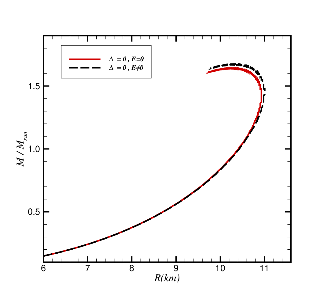
Solving modified TOV equation reveals that adding electric charge makes the radial pressure $p_{r}$ to be increased, as we can see in Fig. 1. But the sensitivity of tangential pressure $p_{t}$ to the electric charge is much more, so $\Delta$ raises up in charged case as is apparent from Fig. 2. This behavior is not only the direct result of our speculation about $p_{r}$ , but also comes from the nature of TOV equation.
Fig. 3 and Fig. 4 refer to uncharged and charged isotropic cases. One may expect adding electric charge to TOV equation causes an increase in the maximum mass of strange quark star $M_{max}$ and also in the corresponding radius $R$ for obtained $M_{max}$ . Since in GR gravitational mass of star and total energy are proportional, adding charge density $\rho_{ch}$ increases the total energy and therefore the above result makes sense. [12]. However, electrical neutrality condition of stars does not allow a significant growth in maximum masses and their corresponding radii.

3.2 Anisotropy Effect

It is shown in Fig. 5 and Fig. 6 that the maximum mass of strange quark star has been raised by adding Gaussian perturbation for obtaining $p_{r}$ . Furthermore, according to Fig. 2 the tangential pressure $p_{t}$ and anisotropy $\Delta$ have a maximum and they do not vanish on the surface. In fact our solution indicate that if there is an anisotropy in the star, it should be maximum on the surface.
Recent measurements indicate that there exist a pulsar of mass 1.97 $\pm$ 0.04 $M_{\odot}$ and this mass rules out nearly all currently proposed equations of state[18]. We have used a trial and error method to get the mentioned mass above. Our calculations indicate that an anisotropy amplitude of $A=3\times 10^{33}Nm^{-2}$ with a standard deviation of $\sigma=3\times 10^{3}m$ and $\mu=\frac{2R}{3}$ in Eq. (18) can survive SQM equation of state which satisfies boundary and hydrostatic equilibrium conditions by $1\%$ and $10\%$ uncertainties at the origin and on the surface respectively as is depicted in Fig. 1.

Refer to caption — Figure 1: Radial pressure $p_{r}$ for various cases: isotropic uncharged, isotropic charged, and anisotropic uncharged matter with $f=5\times 10^{-5}esu$ $g^{-1}$ , $A=3\times 10^{33}Nm^{-2}$ , $\sigma=3\times 10^{3}m$ and $\mu=\frac{2R}{3}$ versus radial coordinate $r$ , all having the same central density of $\rho_{c}=1\times 10^{18}kg$ $m^{-3}$ .

4 Summary

We have studied anisotropic charged strange quark stars with a Gaussian perturbation. Our calculations have shown that the electrical charge effect is much less effective in increasing the maximum mass of star in comparison to anisotropy effect. Also our work has supported that anisotropy can be one of the candidates of describing massive neutron stars with current equations of state.

References

(1) C. Alcock, E. Farhi and A. Olinto, The Astrophysical Journal, 310, 261-272.(1986)
(2) P. Haensel, J. L. Zdunik and R. Schaeffer, A&A, 160, 121.(1986)
(3) E. Farhi and R. L. Jaffe, Physical Review D, 30(11), 2379.(1984)
(4) S. Weinberg, applications of the general theory of relativity, John Wiley and Sons, New York.(1972)
(5) P. Haensel and P. Haensel, EAS Publications Series, 7, 249-249.(2003)
(6) M. K. Mak and T. Harko Chinese Journal of Astronomy and Astrophysics, 248-259.(2002)
(7) T. Singh, G. P. Singh and A. M. Helmi, Il Nuovo Cimento B Series 11, 110(4), 387-393.(1995)
(8) S. Hansraj, S. D. Maharaj and T. Mthethwa, Pramana, 81(4), 557-567.(2013)
(9) M. Ruderman, Annual Review of Astronomy and Astrophysics 10, 427.(1972)
(10) D. Bailin, A. Love, Phys. Rept., 107, 325.(1984)
(11) M. Camenzind, Compact objects in astrophysics, Springer Berlin Heidelberg. (2007)
(12) N. K. Glendenning, Compact Stars, Nuclear Physics, Particle Physics, and General Relativity, Springer. (2000)
(13) P. Haensel, A. Y. Potekhin and D. G. Yakovlev, Neutron stars 1: Equation of state and structure, (Vol. 326). Springer.(2007)
(14) P. S. Negi, International Journal of Modern Physics D, 20(07), 1171-1182. (2011)
(15) S. L. Shapiro and S. A. Teukolsky, Black holes, white dwarfs and neutron stars: the physics of compact objects., John Wiley & Sons. (2008)
(16) R. P. Negreiros, F. Weber, M. Malheiro and V. Usov, Physical Review D, 80(8), 083006. (2009)
(17) S. Ray, A. L. Espindola, M. Malheiro, J. P. Lemos and V. T. Zanchin, Physical Review D, 68(8), 084004. (2003)
(18) P. B. Demorest, T. Pennucci, S. M. Ransom, M. S. E. Roberts and J. W. T. Hessels, Nature, 467(7319), 1081-1083. (2010)