ROBUS: Fair Cache Allocation for Multi-tenant Data-parallel Workloads
Abstract
Systems for processing big data—e.g., Hadoop, Spark, and massively parallel databases—need to run workloads on behalf of multiple tenants simultaneously. The abundant disk-based storage in these systems is usually complemented by a smaller, but much faster, cache. Cache is a precious resource: Tenants who get to use cache can see two orders of magnitude performance improvement. Cache is also a limited and hence shared resource: Unlike a resource like a CPU core which can be used by only one tenant at a time, a cached data item can be accessed by multiple tenants at the same time. Cache, therefore, has to be shared by a multi-tenancy-aware policy across tenants, each having a unique set of priorities and workload characteristics.
In this paper, we develop cache allocation strategies that speed up the overall workload while being fair to each tenant. We build a novel fairness model targeted at the shared resource setting that incorporates not only the more standard concepts of Pareto-efficiency and sharing incentive, but also define envy freeness via the notion of core from cooperative game theory. Our cache management platform, ROBUS, uses randomization over small time batches, and we develop a proportionally fair allocation mechanism that satisfies the core property in expectation. We show that this algorithm and related fair algorithms can be approximated to arbitrary precision in polynomial time. We evaluate these algorithms on a ROBUS prototype implemented on Spark with RDD store used as cache. Our evaluation on an industry-standard workload shows that our algorithms provide a speedup close to performance optimal algorithms while guaranteeing fairness across tenants.
1 Introduction
Two recent trends in data processing are: (i) the use of multi-tenant clusters for analyzing large and diverse datasets, and (ii) the aggressive use of memory to speed up processing by caching datasets. The growing popularity of systems like Apache Spark [4], SAP HANA [24], Hadoop with Discardable Distributed Memory [1], and Tachyon [45] highlight these trends.
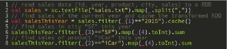
For example, Spark introduces an abstraction called Resilient Distributed Dataset (RDD) to represent any data relevant to modern analytics: files (on a local or distributed file-system), tables (horizontally or vertically partitioned), vertices or edges of graphs, statistical models learned from data, etc. A user can create an RDD directly from data residing on a local or distributed file-system, or by applying a transformation to one or more other RDDs. The user can then direct the system to cache the RDD in memory. Figure 1 gives an example. Computations done on RDDs cached in memory run 10-100x faster than when the data resides on disk [4].
Can User-Directed Caching and Multi-tenancy Coexist? User-directed caching brings some major challenges in a multi-tenant data analytics cluster:
-
A precious resource: Tenants who get to use the in-memory cache see many orders of magnitude of performance improvement. However, the cache is also a limited resource since the total size of memory in a cluster is usually orders of magnitude smaller than the data sizes stored and queried in the cluster.
-
Complications from sharing: Unlike a resource like a CPU core which is used by one tenant at a time, a cached data item can simultaneously benefit a high-priority and a low-priority tenant.
-
Avoiding cache hogs: Low-priority tenants should not be able to hog the available cache, and prevent other tenants from getting the performance benefits they deserve.
-
Utilities differ: Different tenants have different utilities for datasets that could be placed in the cache.
When faced with such challenges, traditional cache allocation policies can lead to user dissatisfaction, poor or unpredictable performance, and low resource utilization. We will illustrate the problems and opportunities through an example. Consider a social-networking company, SpaceBook, that runs a multi-tenant cluster for analyzing datasets about how its users are using the service.
Multiple tenants: The predominant practice in the industry is to group similar users—e.g., users in the same department—into queues (or, pools). Each queue forms a tenant in the cluster. The cluster at SpaceBook is used by three tenants: (i) Analyst, the business analysts in the company, (ii) Engineer, the developers in the company who develop data-driven applications such as recommendation models, and (iii) VP, the top-level management in the company such as the CEO and the Chief Security Officer who look at hourly and daily reports.
Cacheable entities: These three tenants will benefit from caching one or more of three views—R, S, and P—each of size M bytes. Throughout this paper, “view” refers to any data item that can be cached to give a performance benefit. For SQL workloads, a view corresponds to a SQL expression, like any candidate view generated by a materialized view selection algorithm [32, 58, 8, 42]. For broader data analytics—e.g., machine learning and graph processing—a view corresponds to a dataset on which the user has put a cache directive (recall the example Spark program from Figure 1).
| Tenant | |||
|---|---|---|---|
| Analyst | 2 | 1 | 0 |
| Engineer | 2 | 1 | 0 |
| VP | 0 | 1 | 2 |
Utilities: The matrix in Table 1 shows the utility that each tenant gets if the corresponding view were to be cached in memory. A simple definition of utility we will use in this paper is the savings in I/O because data is read from the in-memory cache versus disk. For example, if view R is cached in memory, then tenant Analyst will get a utility of two units. One common pattern in multi-tenant clusters that we bring out in Table 1 is that view R could be the detailed logs that business analysts and developers access quite often; view P could be a table that only the top-level management has access to; while view S could be a materialized view with aggregated information shared by all tenants.
Scenario 1: Debbie, the cluster DBA, is responsible for allocating resources so that the tenants get good performance while all resources are used effectively. Suppose the in-memory cache at SpaceBook has a total size of M bytes. Debbie first configures a static and equal partitioning of the cache so that each tenant is entitled to bytes of cache memory. Recall that each of the views R, S, and P are M bytes each; so none of them will fit in their bytes of cache. Hence, resource utilization will be poor and none of the tenants will receive any performance boost.
Scenario 2: Next, Debbie switches to a more common cache allocation policy, Least Recently Used (LRU). The view R is used the most at Spacebook, so it will likely remain cached for the most time. Thus, the Analyst and Engineer tenants will see performance speedups. However, the VP tenant’s workload will see poor performance, causing these users—including Zuck, SpaceBook’s CEO—to complain that important reports needed for their decision-making are not being generated on time.
Scenario 3: Debbie decides to give the VP tenant 50% higher priority than the other tenants. So, she assigns weights to the Analyst, Engineer, and VP tenants in the ratio . Debbie now switches to a policy that allocates the cache based on the weighted utility of the tenants. She tells Zuck that his reports will now be generated faster. Unfortunately, Zuck will not see any performance improvement: view R will still be the only one cached since it has the highest weighted utility of (); higher than view S’s weighted utility of (), and view P’s weighted utility of ().
Scenario 4: To improve the poor performance seen by the VP tenant, Zuck gives Debbie the money needed to double the cache memory in the cluster. Now two views will fit in the -sized cache. However, even after this massive investment, the VP tenant will only see a minor increase in performance compared to the Analyst and Engineer tenants: views R and S will now be cached since they together have the highest weighted utility of ( for R + for S); higher than for R and P, and for S and P.
Scenario 5: Zuck is very unhappy with Debbie. She now tries to improve things by switching back to static partitioning of for every tenant, causing everyone to get poor performance because none of the views fit. In desperation, Debbie now has to go to the Analyst and Engineer tenants to request them to stop adding cache directives to their workloads. The whole multi-tenant situation becomes extremely messy.
Better scenarios: Let us consider what Debbie would have wanted ideally. An alternative in Scenario 3 is to cache view S instead of R. While S has a slightly lower weighted utility of compared to for , all three tenants will see peformance improvements from caching S. An alternative in Scenario 4 is to cache R and P which will also give performance benefits to all three tenants while only being slightly lower in overall weighted utility than caching R and S. In particular, the VP tenant will now see major benefits from doubling the cache size.
The above example shows non-trivial nature of the problem of cache allocation in multi-tenant setups. There is a need to make principled choices when it comes to picking data items to cache. This motivates the main challenge we address.
Develop a cache allocation policy that provides near-optimal performance speedups for tenants’ workload while simultaneously achieving near-optimal fairness in terms of the tenants’ performance.
Our Contributions.
- •
In Section 2, we propose ROBUS, a platform to optimize multi-tenant query workloads in an online manner using cache for speedup. This framework groups queries in small time-based batches and employs a randomized cache allocation policy on each batch.
- •
In Section 3, we consider the abstract setting of shared resource allocation within a batch, and enumerate properties that we desire from any allocation scheme. We show that the notion of core from cooperative game theory captures the fairness properties in a succinct fashion. We show that when restricted to randomized allocation policies within a batch, a simple algorithm termed proportional fairness generates an allocation which satisfies fairness properties in expectation for that batch.
- •
The policies we construct are based on convex programming formulations of exponential size. Nevertheless, in Section 4, we show that these policies admit to arbitrarily good approximations in polynomial time using the multiplicative weight update method. We present implementations of two fair policies: max-min fairness and proportional fairness. We also present faster and more practical heuristics for computing these solutions.
- •
We show a proof-of-concept implementation of ROBUS on a multi-tenant Spark cluster. Motivated by practical use cases, we develop a synthetic workload generator to create various scenarios. Implementation details and evaluation are provided in Section 5. Results show that our policies provide desirable throughput and fairness in a comprehensive set of setups.
- •
Finally, our policies are specified abstractly, and as such easily extend to other resource allocation settings. We discuss this in Section 3.4.
2 ROBUS Platform
ROBUS (Random Optimized Batch Utility Sharing), shown in Figure 2, is the cache management platform we have developed for multi-tenant data-parallel workloads. ROBUS is designed to be easily pluggable in systems like Hadoop and Spark. Each tenant submits its workload in an online fashion to a designated queue which is characterized by a weight indicating the tenant’s fair share of system resources. (Recall our example from Section 1.)

As illustrated in Figure 2, ROBUS processes the workload in batches by running five steps in a repeated loop. Step 1 removes a batch of queries that were submitted in a fixed time interval into the tenants’ queues. Step 2 runs an algorithm over this entire batch to select a set of views to cache. This computation simultaneously optimizes performance and fairness; designing this algorithm is the main focus of this paper.
Step 2 takes three inputs: (i) a set of candidate views for the query batch, (ii) a utility estimation model for cached views, and (iii) the total cache budget (i.e., memory available for caching). The candidate view generation in ROBUS is a pluggable module. By default, the candidate views for a SQL query are the base tables accessed by the query. For workloads like machine learning and graph processing, the candidate views are datasets on which the user has put a cache directive (recall the example Spark program from Figure 1).
Any candidate view selection algorithm from the literature can be plugged in to ROBUS [32, 58, 8, 42]. To support this feature, ROBUS has a pluggable Step 4 where a query can be rewritten to use the views selected for caching in Step 2 before being run in Step 5. We make use of ROBUS’s pluggability in Section 5 to run a candidate view selection algorithm that considers different vertical projections of input tables in the workload. In future, we plan to extend Step 4 to support re-optimization of the query based on the cached views. Re-optimization may change the query plan entirely.
The utility estimation model is used in the view selection procedure to estimate the utility provided to a query by any cached view. ROBUS currently models these utilities as savings in disk I/O costs if the view were to be read off of in-memory cache versus disk. This approach keeps the models simple and widely applicable. In future, we plan to incorporate richer utility models from the literature that can account for more complex candidate view selection algorithms that consider interactions among views (e.g., use of views can completely change the query plan for a query [44]). Total utility of a cache configuration to a tenant is computed by summing up estimated utilities of the queries submitted by the tenant. The tenant utilities thus computed are used by view selection algorithm to recommend optimal set of views to cache.
In Step 3, the cache is updated with the views selected by our algorithm (if they are not already in the cache). The query batch is then run via Steps 4 and 5. Every query runs as data-parallel tasks in a system like Hadoop or Spark. Our current prototype of ROBUS runs on Spark. A task scheduler (e.g., [2, 27]) is responsible for allocating system resources to the tasks. Cluster memory is divided into two parts: a heap space for run-time objects and a cache for the selected views. While the heap is divided across tasks and is allocated by the task scheduler, the cache is shared by all the queries in the batch simultaneously and managed by ROBUS.
3 Fairness Properties and Policies for Single Batch
In this section we study various notions of fairness when restricted to view selection for queries from a single batch. We consider policies that compute allocations that simultaneously provide large utility to many tenants, and enforce a rigorous notion of fairness between the tenants. Since this is very related to other resource allocation problems in economics [18, 6, 16], we draw heavily on that work for inspiration. However, the key difference from standard resource allocation problems is that in our setting, the resources (or views) are simultaneously shared by tenants. In contrast, the resource allocation settings in economics have typically considered partitioning resources between tenants. As we shall see below, this leads to interesting differences in the notions of fairness.
3.1 Fairness and Randomization
It is well-known in economics [19] that the combination of fairness and indivisible resources (in our case, the cache and views) necessitates randomization. To develop intuition, we present two examples.
First consider a simple fair allocation scheme that for tenants simply allows each tenant to use of the total cache for her preferred view(s). It is plausible that some tenants prefer a large view that does not fit in this partition but does fit in the cache. Therefore, letting tenants have probability of using the whole cache can have arbitrarily larger expected utility than the scheme which with probability 1 lets them use fraction of the whole cache.
Next, consider a batch wherein two tenants each request a different large view such that only one can fit into the cache. In this case, there can be no deterministic allocation scheme that does not ignore one of the tenants. Using randomization, we can easily ensure that each tenant has the same utility in expectation. In fact, utility in expectation will be the per batch guarantee we seek, which over the long time horizon of a workload will lead to deterministic fairness.
Notation for Single Batch
Since our view selection policy works on individual batches at a time, the notation and discussion below is specific to queries within a batch. Let denote the total number of tenants. Define:
Definition 1
A configuration is the set of views feasible in that the sum of the view sizes is at most the cache size.
denotes the utility to tenant that would result from caching , which is defined as the sum over all queries in ’s queue of the utility for that query.
ROBUS generates a set of configurations which by definition can fit in the cache, and assigns a probability to cache each configuration . Define the vector of all such probabilities as:
Definition 2
An Allocation is the vector corresponding to probabilities of choosing configuration normalized so .
We denote as the expected utility of tenant in allocation . ROBUS implements allocation by sampling a configuration from the probability distribution.
For each tenant , let denote the maximum possible utility tenant can obtain if it were the only tenant in the system. For allocation , we define the scaled utility of as . We will use this concept crucially in defining our fairness notions.
3.2 Basic Fairness Desiderata
The first question to ask when designing a fair allocation algorithm is what properties define fairness. There has been much recent work in economics and computer science on heterogeneous resource allocation problems and we begin by considering the properties that this related work examines [27, 52, 39]. Note that because we work within a randomized model, all of these properties are framed in terms of expected utility of tenants.
- •
Pareto Efficiency (PE): An allocation is Pareto-efficient if no other allocation simultaneously improves the expected utility of at least one tenant and does not decrease the expected utility of any tenant.
- •
Sharing Incentive (SI): This property is termed individual rationality in Economics. For tenants, each tenant should expect higher utility in the shared allocation setting than she would expect from simply always having access to of the resources. Since our allocations are randomized, allocation satisfies SI if for all allocations with and for tenants , . In other words, for all tenants , where is the scaled utility function defined above.
One property that is widely studied in other resource allocation contexts is strategy-proofness on the part of the tenants (the notion that no tenant should benefit from lying). In our case, since the queries are seen by the query optimizer, strategy-proofness is not an issue. The above desiderata also omit envy-freeness (that no tenant should prefer the allocation to another tenant) which is something we revisit later.
We now consider a progression of view selection mechanisms on a single batch from very simple to more sophisticated. As a running example, suppose there is a cache of capacity . There are three views , , or that are demanded by tenants. Each view has unit size, so that we can cache only one view any time. Note that this is a drastically simplified example setup only intended to build intuition about why certain view selection algorithms might fail or are superior to others; our results and experiments do not only have unit views, are not limited to three tenants, and may have arbitrarily complex utilities compared to these examples.
We can summarize the input information our view selection might see in a given batch in a table (e.g., Table 2) where the numbers represent utilities tenants get from the views. An allocation here is a vector of three dimensions and that gives the probabilities in our randomized framework for selecting the views.
| Tenant | R | S | P |
|---|---|---|---|
| A | 1 | 0 | 0 |
| B | 0 | 1 | 0 |
| C | 0 | 0 | 1 |
Static Partitioning
Recall that static partitioning is the algorithm that simply deterministically allows each of the tenants to use of the shared resource. This algorithm does not take advantage of randomization. For the example in Table 2, this algorithm cannot cache anything because each user only gets to decide on the use of of the cache. The algorithm is sharing incentive in the standard deterministic setting, but is trivially not Pareto efficient and is not sharing incentive in expectation either. As mentioned previously, such examples motivate the randomization framework to start with.
Random Serial Dictatorship
A natural progression from static partitioning is to consider random serial dictatorship (RSD), a mechanism that is widely considered [16, 6] for problems such as house allocation and school choice. We order the tenants in a random permutation. Each tenant sequentially computes the best set of views to cache (in the residual cache space) to maximize its own utility. In the example in Table 2, each tenant gets a chance of picking her preferred resource (since in a random permutation each tenant has a chance of appearing first) so the allocation is , where each tenant has the same utility in expectation. In fact, it is easy to prove that RSD is always SI: Each tenant has chance of being first in the random ordering, so its scaled utility is at least .
However, in contrast with resource partitioning problems, our problem has a shared aspect that RSD fails to capture. For example, consider the situation in Table 3; RSD computes the same allocation as in the example in Table: 2, . However, on this example, though RSD is SI, it is not Pareto-efficient (PE). Tenants A and C have expected utility of 1 (a chance of getting if they come first in the permutation and a chance of getting if B does) and tenant B has expected utility of with this allocation. However, if we used allocation then tenants A, B, and C all have utility 1, which is strictly better for tenant B and as good for tenants A and C. RSD fails to capture the fact that while each tenant may have different top preferences, many tenants may share secondary preferences.
| Tenant | R | S | P |
|---|---|---|---|
| A | 2 | 1 | 0 |
| B | 0 | 1 | 0 |
| C | 0 | 1 | 2 |
Utility Maximization Mechanism
We next consider the mechanism which simply maximizes the total expected utility of an allocation, i.e., . It is easy to check that this mechanism can ignore tenants who do not contribute enough to the overall utility. In other words, it cannot be SI.
Max-min Fairness (MMF)
In this algorithm we combine previous insights to optimize performance subject to fairness constraints to get a mechanism that is both SI and PE. For allocation , let denote the vector of scaled utilities of the tenants. We choose an allocation so that the vector is lexicographically max-min fair. This means the smallest value in is as large as possible; subject to this, the next smallest value is as large as possible, and so on. We present algorithms to compute these allocations in Section 4.
Theorem 1
The MMF mechanism is both PE and SI.
Proof 3.2.
The RSD mechanism guarantees scaled utility of at least to each tenant. Since the MMF allocation is lexicographically max-min, the minimum scaled utility it obtains is at least the minimum scaled utility in RSD, which is at least . To show PE, note that if there were an allocation that yielded at least as large utility for all tenants, and strictly higher utility for one tenant, the new allocation would be lexicographically larger, contradicting the definition of MMF.
| Tenant | R | S |
|---|---|---|
| 1 | 0 | |
| 1 | 0 | |
| … | … | … |
| 0 | 1 |
Consider the example in Table 4. It is easy to see that the MMF value is and can be achieved with an allocation of . This allocation is both SI and PE.
3.3 Envy-freeness and the Core
The above discussion omits one important facet of fairness. A fair allocation has to be envy free, meaning no tenant has to envy how the allocation treats another tenant. In the case where resources are partitioned between tenants, such a notion is easy to define: No tenant must derive higher utility from the allocation to another tenant. However, in our setting, resources (views) are shared between tenants, and the only common factor is the cache space. In any allocation , each tenant derives utility from certain views, and we can term the expected size of these views as the cache share of this user.
One could try to define envy-freeness in terms of cache space as follows: No tenant should be able to improve expected utility by obtaining the cache share of another tenant. But this simply means all tenants have the same expected cache share. Such an allocation need not be Sharing Incentive. Consider the example in Table 5, where each view and has size and the cache has size . The only allocation that equalizes cache share caches entirely. But this is not SI for tenant .
| Tenant | R | S |
|---|---|---|
| 0 | 1 | |
| 100 | 1 |
This motivates taking the utility of tenants into account in defining envy. However, this quickly gets tricky, since the utility can be a complex function of the entire configuration, and not of individual views. In order to develop more insight, we use an analogy to public projects. The tenants are members of a society, who contribute equal amount of tax. The total tax is the cache space. Each view is a public project whose cost is equal to its size. Users derive utility from the subset of projects built (or views cached). In a societal context, users are envious if they perceive an inordinate fraction of tax dollars being spent on making a small number of users happy. In other words, if they perceive a bridge to nowhere being built. Let us revisit the example in Table 4. Here, the MMF allocation sets and ignores the fact that an arbitrarily large number of tenants want R, compared to just one tenant who wants S. If we treat as a school and as a park, an arbitrarily large number of users want a school compared to a park, yet half the money is spent on the school, and half on the park. This will be perceived as unfair on a societal level.
Randomized Core
In order to formalize this intuition, we borrow the notion of core from cooperative game theory and exchange market economics [29, 55, 13, 22]. We treat each user as bringing a rate endowment of to the system. If they were the only user in the system, we would produce an allocation with and maximize their utility. An allocation over all tenants lies in the core if no subset of tenants can deviate and obtain better utilities for all participants by pooling together their rate endowments. More formally,
Definition 3
An allocation is said to lie in the (randomized) core if for any subset of tenants, there is no feasible allocation such that , for which and for at least one .
It is easy to check that any allocation in the core is both SI and PE, by considering sets of size and respectively. In the above example (Table 4), the allocation lies in the core. Tenant gets its SI amount of utility and cache space. The more demanded view is cached by a proportionally larger amount. In societal terms, each user perceives his tax dollars as being spent fairly. Similarly, in the example in Table 5, the allocation lies in the core.
In the context of provisioning public goods, there are two solution concepts that are known to lie in the core: The first, termed a Lindahl equilibrium [25, 46] attempts to find per-tenant prices that implement a Walrasian equilibrium, while the second, termed ratio equilibrium [38] attempts to find per-tenant ratios of cache-shares. However, these concepts are shown to exist using fixed-point theorems, which don’t lend themselves to efficient algorithmic implementations. We sidestep this difficulty by using randomization to our advantage, and show that a simple mechanism finds an allocation in the core.
Proportional Fairness
Definition 4
An allocation is proportionally fair (PF) if it is a solution to:
| (1) |
We show the following theorem using the KKT (Karush-Kuhn-Tucker) conditions [43]. The proof also follows easily from the classic first order optimality condition of PF [50]; however, we present the entire proof for completeness. Subsequently, in Section 4, we show how to compute this allocation efficiently.
Theorem 3.3.
Proportionally fair allocations satisfy the core property.
Proof 3.4.
Let denote the optimal solution to (PF). Let denote the dual variable for the constraint . By the KKT conditions, we have:
Multiplying the first set of identities by and summing them, we have
This fixes the value of . Next, consider a subset of users, with , along with some allocation with . First note that the KKT conditions implied:
Multiplying by and summing, we have:
Therefore,
Therefore, if for some , then there exists for which . This shows that no subset can deviate to improve their utility, so that the (PF) allocation lies in the core.
3.4 Discussion
Our notion of core easily extends to tenants having weights. Suppose tenant has weight . Then an allocation belongs to the core if for all subsets of tenants, there does not exist with such that for all tenants , , and for at least one . The proportional fairness algorithm is modified to maximize subject to .
We note that the PF algorithm finds an allocation in the (randomized) core to any resource allocation game that can be specified as follows: The goal is to choose a randomization over feasible configurations of resources. Each configuration yields an arbitrary utility to each tenant. This model is fairly general. For instance, consider the setting in [27, 52], where resources can be partitioned fractionally between agents, and an agent’s rate (utility) depends on the minimum resource requirement satisfied in any dimension. Suppose we treat each agent as being endowed with fraction of the supply of resources in all dimensions, the above result shows that the (PF) allocation satisfies the property that no subset of users can pool their endowments together to achieve higher rates for all participants.
Utilities under MMF and PF
We now compare the total utility, for the optimal MMF and (PF) solutions. We present results showing that (PF) has larger utility than MMF in certain canonical scenarios. Our first scenario defines the following grouped instance: There are views, each of unit size. The cache also has size . There are groups of tenants; group has tenants all of which want view .
Lemma 3.5.
The total utility of (PF) is at least the total utility of MMF for any grouped instance.
Proof 3.6.
On grouped instances, MMF sets rate for each tenant, yielding a total utility of for tenants. The (PF) algorithm sets rate for all tenants in group . This yields total utility of . Next note that
Noting that , it is now easy to verify that (PF) yields larger utility.
In fact, the ratio of the utilities of MMF and PF is precisely the Jain’s index [37] of the vector . By setting , and , this shows that (PF) can have times larger total utility than MMF. Our next scenario focuses on arbitrary instances with only two tenants.
Lemma 3.7.
For two tenants, the total utility of (PF) is at least the total utility of MMF.
Proof 3.8.
Let the utilities of the two tenants be in (PF) and in MMF. Assume . Since MMF maximizes the minimum utility, we have . Let and , so that . Since is maximized by definition of PF and is an increasing function, we have , so . Since , this implies . Therefore
This shows completing the proof.
Summary of Fairness Properties
In summary, Table 6 shows the fairness properties that hold for all of our candidate algorithms. We abbreviate the properties SI for sharing incentive and PE for pareto efficiency. Based on this analysis, we suggest that proportional fairness is likely to be a preferable view selection algorithm for our ROBUS framework. The theoretical properties of proportional fairness suggest that it should perform fairly and efficiently.
Algorithm SI PE CORE Random Serial Dictatorship ✓ Utility Maximization ✓ Max-Min Fairness ✓ ✓ Proportional Fairness ✓ ✓ ✓
4 Approximately Computing PF and MMF Allocations
In this section, we show that the PF and MMF allocations can be computed to arbitrary precision. We then present fast heuristic algorithms for approximately computing PF and MMF allocations, which we implement in our prototype.
One key issue in computation is that the number of configurations is exponential in the number of views and tenants, so that the convex programming formulations have exponentially many variables. Nevertheless, since the programs have constraints, we use the multiplicative weight method [11, 26] to solve them approximately in time polynomial in and accuracy parameter . These algorithms assume access to a welfare maximization subroutine that we term Welfare.
Definition 5
Given weight vector , Welfare computes a configuration that maximizes weighted scaled utilities, i.e., solves .
The scaled utilities are computed using the tenant utility model described in Section 2. In our presentation, we assume Welfare solves the welfare maximization problem exactly. Our algorithms will make polynomially many calls to Welfare.
Multiplicative Weight Method
We first detail the multiplicative weight method, which will serve as a common subroutine to all our provably good algorithms. This classical framework [11, 26] uses a Lagrangian update to decide feasibility of linear constraints to arbitrary precision.
We first define the generic problem of deciding the feasibility of a set linear constraints: Given a convex set , and an matrix ,
LP: such that ?
Let be an dimensional dual vector for the constraints . We assume the existence of an efficient Oracle of the form:
Oracle .
The Oracle can be interpreted as follows: Suppose we take a linear combination of the rows of , multiplying row by . Suppose we maximize this as a function of , and it turns out to be smaller than . Then, there is no feasible way to satisfy all constraints in , since the feasible solution would make . On the other hand, suppose we find a feasible . Then, we check which constraints are violated by this , and increase the dual multipliers for these constraints. On the other hand, if a constraint is too slack, we decrease the dual multipliers. We iterate this process until either we find a which proves is infeasible, or the process roughly converges.
More formally, we present the Arora-Hazan-Kale (AHK) procedure [11] for deciding the feasibility of LP. The running time is quantified in terms of the Width defined as:
This procedure has the following guarantee [11]:
Theorem 4.9.
If LP is feasible, the AHK procedure never declares infeasibility, and the final satisfies:
4.1 Proportional Fairness
Our algorithm uses the AHK algorithm as a subroutine and considers dual weights to find an additive approximation solution. The primary result is the following theorem:
Theorem 4.10.
An approximation algorithm computes an additive approximation to (PF) with calls to Welfare, and polynomial additional running time.
Proof
For allocation , let . Let denote the optimal value of (PF), and let denote this optimal value. We first present a Lipschitz type condition, whose proof we omit from this version.
Lemma 4.11.
Let satisfy for . Then, for all , .
The proof idea is to use the concavity of the log function to exhibit a convex combination of and whose value exceeds , which is a contradiction. It is therefore sufficient to find to an additive approximation in order to achieve at least half the welfare of (PF) for all tenants. Towards this end, for a parameter , we write (PF) as a feasibility problem PFFeas as follows:
Definition 6
PFFeas decides the feasibility of the constraints
subject to the constraints:
The above formulation is not an obvious one, and is related to virtual welfare approaches recently proposed in Bayesian mechanism design [20, 15]. The key idea is to connect expected values (utility) to their realizations in each configurations via expected value variables, the . The constraints (P2) and (P1) are over expected values, and realizations respectively. The Oracle computation in the multiplicative weight procedure will decouple into optimizing expected value variables over (P2), and optimizing Welfare over (P1) respectively, and both these problems will be easily solvable.
We note that (P2) has additional constraints . These are in order to reduce the width of the constraints (F). Note that otherwise, can take on unbounded values while still being feasible to (P2), and this makes the width of (F) unbounded. The lower bound of on is to control the approximation error introduced. We argue below that these constraints do not change our problem.
Lemma 4.12.
Let denote the optimal value of the proportional fair allocation (PF). Then, PFFeas is feasible if and only if .
Proof 4.13.
In the formulation PFFeas, the quantity is simply the scaled utility of tenant . Consider the proportionally fair allocation . For this allocation, all scaled utilities lie in since the allocation is SI. Therefore, is feasible for PFFeas. On the other hand, if is feasible to PFFeas for , then is also feasible for (PF), contradicting the optimality of .
We will therefore search for the largest for which PFFeas is feasible. Since each , we have . Therefore, obtaining an additive approximation to by binary search requires evaluations of PFFeas for various , assuming constant .
Solving PFFeas. We now fix a value and apply the AHK procedure to decide the feasibility of PFFeas. To map to the description in the AHK procedure, we have , and is the LHS of the constraints (F). We have . Since any , and , the width of (F) is at most . Finally, for small constant , we will set . Therefore, .
For dual weights , the oracle subproblem is the following:
subject to (P1) and (P2). This separates into two optimization problems.
The first sub-problem maximizes subject to satisfying (P1). This is simply Welfare. The second sub-problem is the following:
subject to satisfying (P2). Let denote the dual multiplier to the constraint . Consider the Lagrangian problem:
subject to for all . The optimal solution sets , which is an non-decreasing function of . We check if . If so, we increase till we satisfy the constraint with equality. This parametric search takes polynomial time, and solves the second sub-problem.
The AHK procedure now gives the following guarantee: Either we declare PFFeas is infeasible, or we find such that for all , we have:
Since , the above implies:
so that the value is achievable with the allocation .
Binary Search. To complete the analysis, since PFFeas is feasible, the procedure will never declare infeasibility when run with , and will find an with , yielding an additive approximation. This binary search over takes iterations.
Thus, we arrive at the result of theorem 4.10.
4.2 Max-min Fairness
We present an algorithm SimpleMMF that computes an allocation maximizing . The MMF allocation can be computed by applying this procedure iteratively as in [28]; we omit the simple details from this version. We note that the idea of applying the multiplicative weight method to compute max-min utility also appeared in [21].
We write the problem of deciding feasibility as SimpleMMF:
subject to the constraints:
We have , where . Therefore, the width . Further, we can set . We can now compute from the AHK procedure, so that in order to approximate to a factor of . The procedure is described in Algorithm 2.
In order to compute MMF allocations, we use a similar idea to decide feasibility, except that we have to perform invocations. This blows up the running time to invocations of Welfare.
The algorithm gives the following result:
Theorem 4.14.
An approximation algorithm for SimpleMMF (Algorithm 2) finds a solution such that using calls to Welfare.
4.3 Fast Heuristics
In this section, we present heuristic algorithms that directly work with the exponential size convex programs. We directly implement these algorithms in software to gather our experimental results.
Configuration Pruning
For , generate random -dimensional unit vectors . For each , let be the configuration corresponding to Welfare. Denote this set of configurations by . We restrict the convex programming formulations of PF and MMF to just the set of configurations , and solve these programs directly, as we describe below. The intuition behind doing this pruning step is the following: The approximation algorithms for PF and MMF find convex combinations of configurations that are optimal for Welfare for some ’s that are computed by the multiplicative weight procedure. Instead of this, we generate random such Pareto-optimal configurations, giving sufficient coverage so that each tenant has a high probability of having the maximum weight at least once.
We compared two algorithms for SimpleMMF, one using the multiplicative weight procedure (Algorithm 2), and the other solving the linear program (Program (3) below) restricted to random optimal configurations. When run on 200 batches with five tenants, using 5 weight vectors gives a 10.4% approximation to the objective of SimpleMMF. With 25 random weight vectors, the approximation error is 1.4%, and using 50 random weights, the approximation error drops to 0.6%. This shows that a small set of configurations that are optimal solutions to Welfare for random vectors is sufficient to generate good approximations to our convex programs. In our implementation, we set to be the union of these configurations along with the configurations generated by the SimpleMMF algorithm (Algorithm 2).
Proportional Fairness
We first note that (PF) is equivalent to the following; the proof of equivalence follows from Theorem 3.3, where the dual variable corresponding to the constraint is precisely .
| (2) |
Given a configuration space , we can solve the program (2) using gradient descent, as shown in Algorithm 3. As precomputation, for each configuration , we precompute . Then .
Max-min Fairness
Using the precomputed configuration space , we solve SimpleMMF using the following linear program:
| (3) |
This can be solved using any off-the-shelf LP solver (our implementation uses the open source lpsolve package [14]). In order to compute the MMF allocation, we iteratively compute the lexicographically max-min allocation using the above LP. The details are standard; see for instance [28]. Briefly, in each iteration a value of is computed. All tenants whose rate cannot be increased beyond without decreasing the rate of another tenant are considered saturated and the rate of for these tenants is a constraint in the next iteration of the LP. The solution to the final LP for which all tenants are saturated is the MMF solution.
5 Evaluation
We evaluate cache allocation policies on a variety of practical setups of multi-tenant analytics clusters. The setups may differ in the number of tenants, workload arrival patterns, data access patterns, etc. Some of the example setups are listed below.
-
Analysts: Tenants correspond to various BI analysts in an enterprise that run a similar workload. Some of the datasets are frequently accessed by all tenants suggesting a good opportunity for shared optimization.
-
ETL+Analysts: All analysts have similar data access patterns as above. But additionally, a tenant runs ETL workload that may touch different datasets than the BI tenants.
-
Production+Engineering: Engineering workload is of bursty nature. Depending on the time of day, engineering queues have different amounts of work whereas production queues, running pre-scheduled workflows, have similar amounts of work.
We replicate various combinations of these setups on a small-scale Spark cluster and run controlled experiments using a mix of TPC-H benchmark [tpch] workload and a synthetically generated scan-based workload.
5.1 Setup and Methodology
Figure 2 has presented the architecture of ROBUS. We use Apache Spark [4] to build a system prototype. Spark is a natural choice for the evaluation since it supports distributed memory-based abstraction in the form of Resilient Distributed Datasets (RDDs). In our prototype, a long running Spark context is shared among multiple queues, with each queue corresponding to a tenant. The Spark context has an access to the entire RDD cache in the cluster. Spark’s internal fair share scheduler is configured with a dedicated pool for each queue; the fair share properties of the pool are set proportional to weight of the corresponding queue.
| Spark version | 1.1.1 |
|---|---|
| Number of worker nodes | 10 |
| Instance type of nodes | c3.2xlarge |
| Total number of cores | 80 |
| Executor memory | 80GB |
Table 7 presents our test cluster setup. We generate two types of data to reflect two types of uses observed in typical multi-tenant clusters: (a) A set of 30 datasets with varying sizes each matching schema of the “sales” tables—, , and —from TPC-DS benchmark [5] data, and (b) All TPC-H benchmark [tpch] datasets generated at scale 5.
The first category of data represents raw fact/log data that comes into the cluster from the OLTP/operational databases in a company. This data is processed by synthetically-generated ETL and exploratory SQL queries, each performing scans and aggregations over a dataset. We refer to this category of queries as the Sales workload. Total size of Sales data on disk is 600GB. We create a vertical projection view on each dataset on its most frequently accessed columns and use it whenever possible to answer queries. Sizes of these views when loaded to cache range from 118MB to 3.6GB as can be seen in Figure 3.
The second category represents data in the cluster after it has been processed by ETL. Note that this data is typically much smaller in size compared to fact/log data. In our experiments, this data is queried by standard TPC-H benchmark queries which consist of a suite of business-oriented analytics and involves more complex operations, such as joins, compared to the Sales workload. All of the queries in our evaluation are submitted using SparkSQL APIs.
We set the cache size to 8GB, 10% of the total executor memory, leaving aside the rest as a heap space. Only 6GB of the cache is used to carry out our optimizations in order to avoid memory management issues our Spark installation experienced while evicting from a near-full cache.
The tenant utility model we use to estimate the utility of a cache configuration in our evaluation is based on the observations made from real-life clusters in [9]. If all the datasets that a query needs are cached, then the query is assigned a utility equal to the total size of data it reads; which corresponds to the savings in disk read I/O. Otherwise, we assign a utility of zero. It is observed in [9] that queries do not benefit much from in-memory caching if any part of their working set is not cached.
The workflow is described in Section 2 already. Here we want to add the fact that the cache update phase in our evaluation setup only marks datasets for caching or uncaching using Spark’s cache directives. Spark lazily updates the cache when the first query requesting cached data from the batch is scheduled for execution.
Workload Arrival and Data Access

Figure 4 shows our workload generation process. Several studies have established that query arrival times follow a Poisson distribution [31, 54]. We use the same in our prototype. Previous studies have also indicated that the data accessed by analytical workloads follows a Zipf distribution [31, 53]: A small number of datasets are more popular than others, while there is a long tail of datasets that are only sporadically accessed. To replicate such data access, our synthetic Sales workload generator picks a dataset from a Zipfian distribution provided at the time of configuration and adds grouping and aggregation predicates from a probability distribution defined for the chosen dataset. The TPC-H workload generator, on the other hand, picks a benchmark query from a probability distribution over the queries provided at the time of configuration.
Further, [53] also shows that 90% of recently accessed data is re-accessed within next hour of first access. This makes a lot of sense because users typically want to drill down a dataset further in response to some interesting observation obtained in the previous run. In order to support such scenarios, we pick a small window in time from a Normal distribution. Over this window, a small subset of datasets is chosen from the Zipfian . This subset forms candidates for the duration of the window. Each query to be generated picks one dataset from the candidates uniformly at random. This technique is taken from [31] which terms the values used in local window as “cold” values to differentiate them from globally popular “hot” values. The generated workload still follows the Zipfian globally. The local distribution is optional; If not provided, datasets are picked from Zipfian at all times.
5.2 Performance Metrics
We gather several performance metrics while executing a workload. They are defined next. We emphasize that these metrics are over long time horizons.
- 1.
Throughput. This is simple to define:
(4) - 2.
Fairness Index. For job schedulers, a performance-based fairness index is defined in terms of variance in slowdowns of jobs in a shared cluster compared to a baseline case where every job receives all the resources [34]. As our work is about speeding up queries, we use relative speedups across queries while deriving fairness. The baseline is the case of statically partitioned cache. Here, is the mean speedup for tenant , and is the weight of tenant .
(5) - 3.
Average Cache Utilization. This is simply the average fraction of cache utilized during workload execution.
- 4.
Hit Ratio. The fraction of queries served off cached views.
Some of the other metrics we collect include flow time, mean execution time, mean wait time, and wait time fairness index. They are not included due to space constraints.
5.3 Algorithm Evaluation
In this section, we evaluate four view selection algorithms on various setups. Each algorithm processes a batch of query workload in an offline manner as detailed in Section 2. Section 3 discussed several possible algorithms. Here, we compare the following:
- 1.
Static: Cache is partitioned in proportion to weights of the tenants. We treat this as baseline when evaluating fairness index.
- 2.
MMF: Max-min fairness implementation described in Section 4.3.
- 3.
FastPF: Proportional fairness implementation described in Section 4.3.
- 4.
OptP: The only goal is to optimize for query performance; Workload from a batch is treated as if belonging to a single tenant – a special case of either MMF or FastPF.
In order to compare these algorithms across various settings, we vary the following parameters independently in our experiments.
5.3.1 Effect of data sharing among tenants
To study the impact of different data sharing patterns on the performance of algorithms, we create four different workload distributions: picks queries uniformly at random over a set of 15 TPC-H benchmark queries; create three different Zipf distributions over 30 Sales datasets over which scan-and-aggregation queries are generated. Each of the distributions is skewed towards a different subset of datasets. Using these distributions, we create four test setups allowing different levels of data sharing, as listed in Table 8. The batch size is set to 40 seconds; the inter-query arrival time distribution for all the tenants is given by Poisson(20); and we run 30 batches of workload for every data point.
| Setup | Distributions used by four tenants |
|---|---|
| {, , , } | |
| {, , , } | |
| {, , , } | |
| {, , , } |
Figure 5 shows how different algorithms perform in each of these setups. Throughput goes down with heterogeneity in data access. Static policy fails to cache any dataset for TPC-H workload because each of the queries we generate reads the largest table, lineitem, which amounts to , much larger than cache at the disposal of Static. The other three policies, on the other hand, can serve every query off cache in setup . As a result, they exhibit a throughput of more than 2x over Static. However, as the heterogeneity in data access increases, the gap in throughput narrows. Even though the shared policies cache more data, frequent updates to cache configuration per batch cause additional delays. We explore possibility of retaining state of cache in Section 5.4.
Among the shared cache policies, OptP scores high on throughput but very low on fairness index. It uses cache exclusively for TPC-H tenants at the cost of degradation to Sales tenants’ performance. MMF and FastPF policies, on the other hand show much better tradeoffs in terms of performance and fairness to tenants.
We also repeated the same experiment on Sales data alone. We first create four different Zipf distributions over candidate views: . Each of the distributions is skewed towards a different subset of views.We create four test setups, each allowing a different level of data sharing, as listed in Table 9. The other common parameters are listed in Table 10.
| Setup | Distributions used by four tenants |
|---|---|
| {, , , } | |
| {, , , } | |
| {, , , } | |
| {, , , } |
| Parameter | Value |
|---|---|
| Query inter-arrival rates (sec) | {20 tenant} |
| Batch size (sec) | 40 |
| Number of batches | 30 |
Figure 6 shows how different algorithms perform in each of these setups. Throuphput goes down with heterogeneity in data access. Static performs poorly in all the setups, the performance being between 30%-40% worse of the others. Its lower cache utilization and lower hit ratio are further indicators of why Static is not the right choice for cache allocation. There is very little to distinguish among the three cache-sharing algorithms. This shows that our fair algorithms can provide a throughput close to the optimal. In terms of fairness, OptP algorithm gives the most inconsistent performance. It scores high in the setup with most heterogeneity, but fails when data sharing is involved. MMF and FastPF, on the other hand, score high in all the setups.
The performance of MMF interestingly falls alarmingly low in the second setup. This is clearly an outcome of the data sharing pattern wherein three of four tenants largely share the same subset of views. Recollecting the example presented in Table 4, MMF tries to share the cache (probabilistically) equally between the two sets of tenants effectively producing an allocation off the core. We include a chart showing the duration the most popular views were cached for by MMF, FastPF, and OptP. (Figure 7) Top three views in each of and serve 25%, 13%, and 8% of the queries respectively. It can be seen that while MMF caches the topmost view from the distributions roughly equally, FastPF and OptP favor the topmost view from more since it is shared by three tenants. MMF tries to compensate the three tenants by caching their second best view more, but this view has a lower utility both due to lower access frequency and smaller size. So the overall performance of MMF suffers in this case.
5.3.2 Effect of variance in query arrival rates
To replicate the bursty tenants scenarios, we vary query inter-arrival rates of tenants in a two-tenant setup. We create three setups—low, mid, and high—with query inter-arrival rates as listed in Table 11. The other parameters used in each of the setups are listed in Table 12.
| Setup | Poisson mean, | Poisson mean, |
|---|---|---|
| low | 12 | 12 |
| mid | 18 | 8 |
| high | 24 | 6 |
| Parameter | Value |
|---|---|
| Data access distributions | |
| Batch size (sec) | 72 |
| Number of batches | 30 |
Figure 8 shows the impact of variance in query arrival rate on various metrics. The performance of Static remains below the other three algorithms as can be seen from the first three graphs. The performance gap, however, is small because the cache is partitioned in only two parts for Static each part being large enough to serve 80% of the queries that could be served off unpartitioned cache. When it comes to the fairness index, all the algorithms except OptP get a near-perfect score. OptP favors the faster tenant in both mid and high setups so much that the slower tenant’s performance degrades. Figure 9 shows the speedups for MMF, FastPF, and OptP relative to Static under the setup high. It can be seen that the first tenant sees a performance degradation with OptP empirically proving the fact that OptP is not sharing incentive.
5.3.3 Effect of number of tenants
| Setup | Poisson mean, |
|---|---|
| 2 | 10 |
| 4 | 20 |
| 8 | 40 |
| Parameter | Value |
|---|---|
| Data access distributions | { tenant} |
| Batch size (sec) | 40 |
| Number of batches | 30 |
To further stress the utility of optimizing the entire cache as a shared resource, we experiment with increasing number of tenants. Specifically, we consider scenarios with 2, 4, and 8 tenants, all using the same distribution over dataset access. We try to keep the number of queries per batch the same by doubling query inter-arrival rate with doubling of the number of tenants, batch size remaining the same across the setups. Table 13 lists the query inter-arrival rates we used. The other parameters common across the setups are listed in Table 14.
Figure 10 shows behavior of the algorithms under these scenarios. The gap in throughput between Static and the other algorithms is large (35%-45%). As the number of tenants goes up, the average cache utilization of Static drops sharply, whereas the average cache utilization of the other algorithms remain largely stable. This can be attributed to the static partitioning of cache in Static. The hit ratio shows a similar pattern again showing why Static is not the best choice. In terms of fairness index, OptP finds it increasingly harder to provide a fair solution. With an increase in the number of tenants, the number of queries per tenant per batch goes down which makes the locally optimal choices of OptP more unlikely to provide equal speedups. In contrast, MMF and FastPF, with their randomized choices, score over 0.9 in all the scenarios exhibiting their superiority.
5.4 Discussion and Future Work
Our evaluation on practical setups brings up some interesting insights that opens up multiple possibilities for the future. We discuss some of the challenges and the directions here.
Our experiments show that across all setups, FastPF and MMF provide far better trade-offs in throughput and fairness compared to Static and OptP. We note that in comparing max-min fair and proportional fair implementations, there is no clear winner. We believe this is a second order difference that a more precise cost model and implementations of the exact algorithms (for instance, the algorithm in Section 4.1 for proportional fairness) will bring out. However, even given similar empirical results, PF has the advantage of the core property as a succinct and easy to explain notion of fairness.
We next note that the running time of our algorithms is polynomial in number of tenants. In most typical industry setups, the ones we evaluated, there is only a handful number of tenants. Therefore, we expect our algorithms to be fast even in the wild. Just to quantify the query wait times, we observed them to be of the order of tens of milliseconds in most cases.
Convergence Properties
As our algorithms are randomized in nature, it is important to study how long they take to converge to solutions that yield fairness across time. After running several workloads, we find that the number of batches to achieve convergence is very small, of the order of 15-25. In Figure 11, we present results of a four tenant workload with 50 batches, optimized once using MMF and once using FastPF. The fairness index was computed after every 2-4 batches. It can be seen that both algorithms converge to their respective optimal values at around 20 batches. As a future work, we plan to systematically study which parameters define rate of convergence of the algorithms.
Batch Size and Cache State
Our batched processing architecture introduces additional optimization choices. Primarily, there are two ways of tuning a view selection algorithm:
1. Controlling batch size, and
2. Managing state of cache across batches.
The first option needs no elaboration. The second option is whether the cache is treated as stateful or as stateless when optimizing a batch. In the former case, the estimated benefit of views that are already in cache is boosted by a factor . This influences the next cache allocation, and makes it more likely for these views to stay in the cache. The latter case ignores the state of the cache when considering the next batch. All the results presented so far have used stateless cache.
We empirically compared how the algorithms react to these parameters. Figure 12 shows effect of change in batch size on two versions each of MMF and FastPF: one treating the cache as stateless (MMFsl and FastPFsl), and the other treating it as stateful (MMFsf and FastPFsf), with . It can be seen that both versions provide similar throughput in all the cases. It can be observed that the stateful algorithms score higher on fairness for the smallest batch size but there is no clear pattern seen when the batch size is larger. It makes sense since the lower batch sizes do not give enough choices for fair configurations of cache and maintaining the state results in an artificial increase of the batch size thereby providing better configurations. As a future work, we plan to explore these trade-offs on a larger scale to devise better guidelines on parameter tuning.
Engineering issues
We now highlight some challenges in scaling up our experiments to industry scale. These challenges are tied to engineering issues in current implementations of systems such as Spark, and will get ironed out over time. Most common multi-tenant Spark setups use a separate Spark context for each tenant, effectively partitioning cache. In fact, most current multi-tenant data warehouse systems recommend splitting memory across queues. This is in part due to multi-thread management challenges that result in unpredictable behavior such as premature eviction of cached data blocks. Another engineering issue, specific to Spark, is the inordinately long delays in garbage collection when cluster scales up. We should be able to see a much better impact of ROBUS optimization once these practical issues get resolved.
Code Base
The code base of ROBUS has been open-sourced [3] and our entire experimental setup can be replicated following a simple set of instructions provided with the code.
6 Related Work
Physical design tuning and Multi-query optimization
Classical view materialization algorithms in databases [32, 58, 8, 30, 47] treat entire workload as a set and optimize towards one or more of the flow time, space budget, and view maintenance costs. Online physical design tuning approaches [17, 42, 23, 44], on the other hand, adapt to changes in query workload by modifying physical design. None of the afore-mentioned approaches support multi-tenant workloads and therefore cannot be used in selecting views for caching. However, some of the techniques used, in particular candidate view enumeration, view matching, and query rewrite, can be applied in ROBUS framework.
Fairness theory
The proportional fairness algorithm is widely studied in Economics [50, 36, 18] as well as in scheduling theory [27, 52, 41, 40, 33, 57, 10]. In the context of resource partitioning problems (or exchange economies) [13, 22], it is well-known that a convex program, called the Eisenberg-Gale convex program [36] computes prices that implement a Walrasian equilibrium (or market clearing solution). Our shared resource allocation problem is different from allocation problems where resources need to be partitioned, and it is not clear how to specify prices for resources (or views) in our setting. Nevertheless, we show that there is an exponential size convex program using configurations as variables, whose solution implements proportional fairness in a randomized sense.
In scheduling theory, the focus is on analyzing delay properties [41, 40, 33] assuming jobs have durations. Our focus is instead on utility maximization, which has also been considered in the context of wireless scheduling in [57, 10]. The latter work focuses on long-term fairness for partitioned resources, where utility of a tenant is defined as sum of discounted utilities across time. The resulting algorithms, though simple, only provide guarantees assuming job arrivals are ergodic, and if tenants exist forever. They do not provide per-epoch guarantees. In contrast, we focus on obtaining per-epoch fairness in a randomized sense without ergodic assumptions, and on defining the right fairness concepts when resources are shared. We finally note that [39] presents dynamic schemes for achieving envy-freeness across time; however, these techniques are specific to resource partitioning problems and to not directly apply to our shared resource setting.
Multi-tenant architectures
Traditionally, the notion of multi-tenancy in databases deals with sharing database system resources, viz. hardware, process, schema, among users [35, 12, 48]. Each tenant only accesses data owned by them. Emerging multi-tenant big data architectures, on the other hand, allow for entire cluster data to be shared among tenants. This sharing of data is critical in our work as it allows the cache to be used much more efficiently.
A critical component of modern multi-tenant architectures, such as Apache Hadoop, Apache Spark, Cloudera Impala, is a fair scheduler/ resource allocator [2, 27, 34]. The resource pool considered by these schedulers do not differentiate the cache resource from the heap resource and as a result divides the cache among tenants. As seen in our work, partitioned cache setups severely reduce optimization opportunities. Some recent approaches treat cache as an independent resource when running multiple jobs. PACMan [9] exploits multi-wave execution workflow of Hadoop jobs to make caching decisions at the granularity of parallely running tasks of a job. In another work, LRU policies for Buffer pool memory are extended to meet SLA guarantees of multiple tenants [49]. However, none of the approaches exploit the opportunities presented by multi-shared nature of cache resource. In another advancement, distributed analytics systems are supporting a distributed cache store shared by multiple tenants [45, 1]. ROBUS optimizer will be a natural fit for such systems.
7 Conclusion
Emerging Big data multi-tenant analytics systems complement an abundant disk-based storage with a smaller, but much faster, cache in order to optimize workloads by materializing views in the cache. The cache is a shared resource, i.e., cached data can be accessed by all tenants. In this paper, we presented ROBUS, a cache management platform for achieving both a fair allocation of cache and a near-optimal performance in such architectures. We defined notions of fairness for the shared settings using randomization in small batches as a key tool. We presented a fairness model that incorporates Pareto-efficiency and sharing incentive, and also achieves envy-freeness via the notion of core from cooperative game theory. We showed a proportionally fair mechanism to satisfy the core property in expectation. Further, we developed efficient algorithms for two fair mechanisms and implemented them in a ROBUS prototype built on a Spark cluster. Our experiments on various practical setups show that it is possible to achieve near-optimal fairness, while simultaneously preserving near-optimal performance speedups using the algorithms we developed.
Our framework is quite general and applies to any setting where resource allocations are shared across agents. As future work, we plan to explore other applications of this framework.
References
- [1] Discardable distributed memory: Supporting memory storage in HDFS, http://hortonworks.com/blog/ddm/.
- [2] Hadoop fair scheduler, http://hadoop.apache.org/docs/r1.2.1/fair_scheduler.html.
- [3] ROBUS Cache Planner, https://github.com/dukedbgroup/ROBUS.
- [4] Spark: Lightning fast cluster computing, https://spark.apache.org/.
- [5] TPC-DS benchmark, http://www.tpc.org/tpcds/.
- [6] A. Abdulkadiroglu and T. Sonmez. Random serial dictatorship and the core from random endowments in house allocation problems. Econometrica, 66(3):689–701, 1998.
- [7] P. Agrawal, D. Kifer, and C. Olston. Scheduling shared scans of large data files. Proc. VLDB Endow., 1(1):958–969, Aug. 2008.
- [8] S. Agrawal, S. Chaudhuri, and V. R. Narasayya. Automated selection of materialized views and indexes in SQL databases. In Proceedings of the 26th International Conference on Very Large Data Bases, VLDB ’00, pages 496–505, San Francisco, CA, USA, 2000. Morgan Kaufmann Publishers Inc.
- [9] G. Ananthanarayanan, A. Ghodsi, A. Wang, D. Borthakur, S. Kandula, S. Shenker, and I. Stoica. PACMan: Coordinated memory caching for parallel jobs. In Proceedings of the 9th USENIX Conference on Networked Systems Design and Implementation, NSDI’12, pages 20–20, Berkeley, CA, USA, 2012. USENIX Association.
- [10] M. Andrews. Instability of the proportional fair scheduling algorithm for hdr. Wireless Communications, IEEE Transactions on, 3(5):1422–1426, 2004.
- [11] S. Arora, E. Hazan, and S. Kale. The multiplicative weights update method: A meta algorithm and applications. Theory of Computing, 8:121–164, 2005.
- [12] S. Aulbach, T. Grust, D. Jacobs, A. Kemper, and J. Rittinger. Multi-tenant databases for software as a service: Schema-mapping techniques. In Proceedings of the 2008 ACM SIGMOD International Conference on Management of Data, SIGMOD ’08, pages 1195–1206, New York, NY, USA, 2008. ACM.
- [13] R. J. Aumann. Markets with a continuum of traders. Econometrica: Journal of the Econometric Society, pages 39–50, 1964.
- [14] M. Berkelaar, K. Eikland, and P. Notebaert. lpsolve : Open source (Mixed-Integer) Linear Programming system.
- [15] A. Bhalgat, S. Gollapudi, and K. Munagala. Optimal auctions via the multiplicative weight method. In Proceedings of the fourteenth ACM conference on Electronic commerce, pages 73–90. ACM, 2013.
- [16] A. Bogomolnaia and H. Moulin. A new solution to the random assignment problem. Journal of Economic Theory, 100(2):295–328, 2001.
- [17] N. Bruno and S. Chaudhuri. An online approach to physical design tuning. In Proceedings of the International Conference on Data Engineering (ICDE), 2007.
- [18] E. Budish. The combinatorial assignment problem: Approximate competitive equilibrium from equal incomes. Journal of Political Economy, 119(6):1061–1103, 2011.
- [19] E. Budish, Y.-K. Che, F. Kojima, and P. Milgrom. Designing random allocation mechanisms: Theory and applications. American Economic Review, 103(2):585–623, 2013.
- [20] Y. Cai, C. Daskalakis, and S. M. Weinberg. Optimal multi-dimensional mechanism design: Reducing revenue to welfare maximization. In FOCS, 2012.
- [21] D. Chakrabarty, A. Mehta, and V. Vazirani. Design is as easy as optimization. In M. Bugliesi, B. Preneel, V. Sassone, and I. Wegener, editors, Automata, Languages and Programming, volume 4051 of Lecture Notes in Computer Science, pages 477–488. Springer Berlin Heidelberg, 2006.
- [22] G. Debreu and H. Scarf. A limit theorem on the core of an economy. International Economic Review, 4(3):pp. 235–246, 1963.
- [23] I. Elghandour and A. Aboulnaga. Restore: Reusing results of mapreduce jobs. Proc. VLDB Endow., 5(6):586–597, Feb. 2012.
- [24] F. Färber, S. K. Cha, J. Primsch, C. Bornhövd, S. Sigg, and W. Lehner. Sap hana database: Data management for modern business applications. SIGMOD Rec., 40(4):45–51, Jan. 2012.
- [25] D. K. Foley. Lindahl’s solution and the core of an economy with public goods. Econometrica: Journal of the Econometric Society, pages 66–72, 1970.
- [26] Y. Freund and R. E. Schapire. Adaptive game playing using multiplicative weights. Games and Economic Behavior, 29(1–2):79 – 103, 1999.
- [27] A. Ghodsi, M. Zaharia, B. Hindman, A. Konwinski, S. Shenker, and I. Stoica. Dominant resource fairness: Fair allocation of multiple resource types. In Proceedings of the 8th USENIX Conference on Networked Systems Design and Implementation, NSDI’11, pages 323–336, Berkeley, CA, USA, 2011. USENIX Association.
- [28] A. Ghodsi, M. Zaharia, S. Shenker, and I. Stoica. Choosy: Max-min fair sharing for datacenter jobs with constraints. In Proceedings of the 8th ACM European Conference on Computer Systems, pages 365–378. ACM, 2013.
- [29] D. Gillies. Some Theorems on n-Person Games. PhD thesis, Princeton University, 1953.
- [30] J. Goldstein and P.-A. Larson. Optimizing queries using materialized views: A practical, scalable solution. In Proceedings of the 2001 ACM SIGMOD International Conference on Management of Data, SIGMOD ’01, pages 331–342, New York, NY, USA, 2001. ACM.
- [31] J. Gray, K. Baclawski, P. Sundaresan, and S. Englert. Quickly generating billion-record synthetic databases. Association for Computing Machinery, Inc., January 1994.
- [32] H. Gupta and I. S. Mumick. Selection of views to materialize in a data warehouse. IEEE Transactions on Knowledge and Data Engineering, 17(1):24–43, 2005.
- [33] S. Im, J. Kulkarni, and K. Munagala. Competitive algorithms from competitive equilibria: Non-clairvoyant scheduling under polyhedral constraints. In Proceedings of the 46th Annual ACM Symposium on Theory of Computing, STOC ’14, pages 313–322, 2014.
- [34] M. Isard, V. Prabhakaran, J. Currey, U. Wieder, K. Talwar, and A. Goldberg. Quincy: Fair scheduling for distributed computing clusters. In Proceedings of the ACM SIGOPS 22Nd Symposium on Operating Systems Principles, SOSP ’09, pages 261–276, New York, NY, USA, 2009. ACM.
- [35] D. Jacobs, S. Aulbach, and T. U. München. Ruminations on multi-tenant databases. In BTW Proceedings, volume 103 of LNI, pages 514–521. GI, 2007.
- [36] K. Jain and V. V. Vazirani. Eisenberg-gale markets: Algorithms and structural properties. In Proceedings of the thirty-ninth annual ACM symposium on Theory of computing, pages 364–373. ACM, 2007.
- [37] R. K. Jain, D.-M. W. Chiu, and W. R. Hawe. A quantitative measure of fairness and discrimination for resource allocation in shared computer systems. Technical report, Digital Equipment Corporation, Sept. 1984.
- [38] M. Kaneko. The ratio equilibrium and a voting game in a public goods economy. Journal of Economic Theory, 16(2):123–136, 1977.
- [39] I. Kash, A. D. Procaccia, and N. Shah. No agent left behind: Dynamic fair division of multiple resources. In Proceedings of the 2013 International Conference on Autonomous Agents and Multi-agent Systems, AAMAS ’13, pages 351–358, Richland, SC, 2013. International Foundation for Autonomous Agents and Multiagent Systems.
- [40] F. Kelly, L. Massoulié, and N. Walton. Resource pooling in congested networks: proportional fairness and product form. Queueing Systems, 63(1-4):165–194, 2009.
- [41] F. P. Kelly, A. K. Maulloo, and D. K. H. Tan. Rate control for communication networks: Shadow prices, proportional fairness and stability. The Journal of the Operational Research Society, 49(3):pp. 237–252, 1998.
- [42] Y. Kotidis and N. Roussopoulos. DynaMat: A dynamic view management system for data warehouses. In Proceedings of the 1999 ACM SIGMOD International Conference on Management of Data, SIGMOD ’99, pages 371–382, New York, NY, USA, 1999. ACM.
- [43] H. W. Kuhn and A. W. Tucker. Nonlinear programming. In Proceedings of the Second Berkeley Symposium on Mathematical Statistics and Probability, pages 481–492, Berkeley, Calif., 1951. University of California Press.
- [44] J. LeFevre, J. Sankaranarayanan, H. Hacigumus, J. Tatemura, N. Polyzotis, and M. J. Carey. Miso: Souping up big data query processing with a multistore system. In Proceedings of the 2014 ACM SIGMOD International Conference on Management of Data, SIGMOD ’14, pages 1591–1602, New York, NY, USA, 2014. ACM.
- [45] H. Li, A. Ghodsi, M. Zaharia, E. Baldeschwieler, S. Shenker, and I. Stoica. Tachyon: Memory throughput I/O for cluster computing frameworks. LADIS, 18:1, 2013.
- [46] A. Mas-Colell and J. Silvestre. Cost share equilibria: A lindahlian approach. Journal of Economic Theory, 47(2):239–256, 1989.
- [47] H. Mistry, P. Roy, S. Sudarshan, and K. Ramamritham. Materialized view selection and maintenance using multi-query optimization. In Proceedings of the 2001 ACM SIGMOD International Conference on Management of Data, SIGMOD ’01, pages 307–318, New York, NY, USA, 2001. ACM.
- [48] V. Narasayya, S. Das, M. Syamala, S. Chaudhuri, F. Li, and H. Park. A demonstration of SQLVM: Performance isolation in multi-tenant relational database-as-a-service. In Proceedings of the 2013 ACM SIGMOD International Conference on Management of Data, SIGMOD ’13, pages 1077–1080, New York, NY, USA, 2013. ACM.
- [49] V. Narasayya, I. Menache, M. Singh, F. Li, M. Syamala, and S. Chaudhuri. Sharing buffer pool memory in multi-tenant relational database-as-a-service. Proc. VLDB Endow., 8(7):726–737, Feb. 2015.
- [50] J. Nash. The bargaining problem. Econometrica, 18(2):155–162, 1950.
- [51] T. Nykiel, M. Potamias, C. Mishra, G. Kollios, and N. Koudas. MRShare: Sharing across multiple queries in mapreduce. Proc. VLDB Endow., 3(1-2):494–505, Sept. 2010.
- [52] D. C. Parkes, A. D. Procaccia, and N. Shah. Beyond dominant resource fairness: Extensions, limitations, and indivisibilities. In Proceedings of the 13th ACM Conference on Electronic Commerce, EC ’12, pages 808–825, New York, NY, USA, 2012. ACM.
- [53] K. Ren, Y. Kwon, M. Balazinska, and B. Howe. Hadoop’s adolescence: An analysis of hadoop usage in scientific workloads. Proc. VLDB Endow., 6(10):853–864, Aug. 2013.
- [54] Z. Ren, X. Xu, J. Wan, W. Shi, and M. Zhou. Workload characterization on a production hadoop cluster: A case study on Taobao. In IISWC’12, pages 3–13, 2012.
- [55] H. E. Scarf. The core of an n person game. Econometrica, 35(1):pp. 50–69, 1967.
- [56] T. K. Sellis. Multiple-query optimization. ACM Trans. Database Syst., 13(1):23–52, Mar. 1988.
- [57] A. L. Stolyar. On the asymptotic optimality of the gradient scheduling algorithm for multiuser throughput allocation. Oper. Res., 53(1):12–25, 2005.
- [58] J. Yang, K. Karlapalem, and Q. Li. Algorithms for materialized view design in data warehousing environment. In Proceedings of the 23rd International Conference on Very Large Data Bases, VLDB ’97, pages 136–145, San Francisco, CA, USA, 1997. Morgan Kaufmann Publishers Inc.
- [59] M. Zukowski, S. Héman, N. Nes, and P. Boncz. Cooperative scans: Dynamic bandwidth sharing in a dbms. In Proceedings of the 33rd International Conference on Very Large Data Bases, VLDB ’07, pages 723–734. VLDB Endowment, 2007.
Appendix A Experiment results
A.1 Results of experiments on effect of data sharing on mixed workload
| Metric | Static | MMF | FastPF | OptP |
|---|---|---|---|---|
| Throughput(/min) | 7.80 | 19.2 | 19.2 | 19.2 |
| Avg cache util. | 0.00 | 0.83 | 0.83 | 0.83 |
| Hit ratio | 0.00 | 1.00 | 1.00 | 1.00 |
| Fairness index | 1.00 | 0.71 | 0.71 | 0.71 |
| Metric | Static | MMF | FastPF | OptP |
|---|---|---|---|---|
| Throughput(/min) | 7.20 | 9.00 | 10.2 | 16.2 |
| Avg cache util. | 0.08 | 0.81 | 0.87 | 0.92 |
| Hit ratio | 0.08 | 0.54 | 0.68 | 0.83 |
| Fairness index | 1.00 | 0.83 | 0.79 | 0.75 |
| Metric | Static | MMF | FastPF | OptP |
|---|---|---|---|---|
| Throughput(/min) | 7.20 | 7.50 | 7.80 | 9.60 |
| Avg cache util. | 0.16 | 0.96 | 0.98 | 1.00 |
| Hit ratio | 0.19 | 0.53 | 0.55 | 0.67 |
| Fairness index | 1.00 | 0.77 | 0.66 | 0.50 |
| Metric | Static | MMF | FastPF | OptP |
|---|---|---|---|---|
| Throughput(/min) | 5.40 | 5.40 | 5.40 | 4.80 |
| Avg cache util. | 0.24 | 0.91 | 0.93 | 0.96 |
| Hit ratio | 0.26 | 0.43 | 0.47 | 0.46 |
| Fairness index | 1.00 | 0.81 | 0.80 | 0.38 |
A.2 Results of experiments on effect of data sharing on Sales workload
| Metric | Static | MMF | FastPF | OptP |
|---|---|---|---|---|
| Throughput(/min) | 6.00 | 9.42 | 9.42 | 10.08 |
| Avg cache util. | 0.34 | 0.87 | 0.86 | 0.88 |
| Hit ratio | 0.42 | 0.67 | 0.67 | 0.68 |
| Fairness index | 1.00 | 0.98 | 0.94 | 0.84 |
| Metric | Static | MMF | FastPF | OptP |
|---|---|---|---|---|
| Throughput(/min) | 5.70 | 7.20 | 7.44 | 8.24 |
| Avg cache util. | 0.34 | 0.93 | 0.90 | 0.94 |
| Hit ratio | 0.43 | 0.57 | 0.61 | 0.63 |
| Fairness index | 1.00 | 0.96 | 0.92 | 0.78 |
| Metric | Static | MMF | FastPF | OptP |
|---|---|---|---|---|
| Throughput(/min) | 5.34 | 7.44 | 7.38 | 7.92 |
| Avg cache util. | 0.30 | 0.93 | 0.93 | 0.94 |
| Hit ratio | 0.38 | 0.60 | 0.59 | 0.58 |
| Fairness index | 1.00 | 0.98 | 0.92 | 0.72 |
| Metric | Static | MMF | FastPF | OptP |
|---|---|---|---|---|
| Throughput(/min) | 4.20 | 5.64 | 5.76 | 6.00 |
| Avg cache util. | 0.28 | 0.89 | 0.88 | 0.92 |
| Hit ratio | 0.34 | 0.50 | 0.56 | 0.55 |
| Fairness index | 1.00 | 0.96 | 0.96 | 0.99 |
A.3 Results of experiments on effect of query arrival rate
| Metric | Static | MMF | FastPF | OptP |
|---|---|---|---|---|
| Throughput(/min) | 5.76 | 6.42 | 6.72 | 6.90 |
| Avg cache util. | 0.77 | 0.93 | 0.93 | 0.94 |
| Hit ratio | 0.40 | 0.50 | 0.49 | 0.51 |
| Fairness index | 1.00 | 1.00 | 0.99 | 0.97 |
| Metric | Static | MMF | FastPF | OptP |
|---|---|---|---|---|
| Throughput(/min) | 6.12 | 6.78 | 6.96 | 6.96 |
| Avg cache util. | 0.72 | 0.90 | 0.89 | 0.90 |
| Hit ratio | 0.44 | 0.49 | 0.49 | 0.56 |
| Fairness index | 1.00 | 1.00 | 0.98 | 0.87 |
| Metric | Static | MMF | FastPF | OptP |
|---|---|---|---|---|
| Throughput(/min) | 5.52 | 6.12 | 6.30 | 6.54 |
| Avg cache util. | 0.69 | 0.90 | 0.91 | 0.91 |
| Hit ratio | 0.39 | 0.48 | 0.48 | 0.51 |
| Fairness index | 1.00 | 1.00 | 1.00 | 0.89 |
A.4 Results of experiments on effect of number of tenants
| Metric | Static | MMF | FastPF | OptP |
|---|---|---|---|---|
| Throughput(/min) | 7.00 | 10.00 | 9.70 | 10.40 |
| Avg cache util. | 0.67 | 0.93 | 0.93 | 0.97 |
| Hit ratio | 0.50 | 0.68 | 0.68 | 0.68 |
| Fairness index | 1.00 | 0.98 | 1.00 | 1.00 |
| Metric | Static | MMF | FastPF | OptP |
|---|---|---|---|---|
| Throughput(/min) | 6.00 | 9.40 | 9.40 | 10.10 |
| Avg cache util. | 0.34 | 0.87 | 0.86 | 0.88 |
| Hit ratio | 0.42 | 0.67 | 0.67 | 0.68 |
| Fairness index | 1.00 | 0.98 | 0.94 | 0.84 |
| Metric | Static | MMF | FastPF | OptP |
|---|---|---|---|---|
| Throughput(/min) | 5.34 | 8.34 | 8.22 | 9.18 |
| Avg cache util. | 0.07 | 0.82 | 0.82 | 0.87 |
| Hit ratio | 0.26 | 0.65 | 0.65 | 0.68 |
| Fairness index | 1.00 | 0.94 | 0.91 | 0.78 |