Approximate Fitting of a Circular Arc
When Two Points Are Known

The purpose of this paper is to solve fitting a circular arc to a set of points (or segments) with complexity $\displaystyle O{\left(1\right)}$ when two points on the arc and moments up to the fourth order are known.

In papers [3] and [4], fitting a circle is done by finding a circle with center $\displaystyle(x_{c},y_{c})$ and radius $\displaystyle r$, which minimizes the next equation

where $\displaystyle(x_{i},y_{i})$ are $\displaystyle i$-th point, $\displaystyle i=\overline{1..n}$.

This formula minimizes the squared differences between squared distances from the circle center to the points and square of the radius. The solution is found by using only the moments of $\displaystyle(x_{i},y_{i})$ with complexity $\displaystyle O{\left(1\right)}$. However, this leads to bias in the estimation of parameters [3, see pp. 368-370]. Suppose that each point has been fitted with $\displaystyle\epsilon_{i}$ error. Substituting it in (1) gives

Assuming that $\displaystyle\epsilon_{i}$ are small compared to radius $\displaystyle r$ and neglecting higher orders

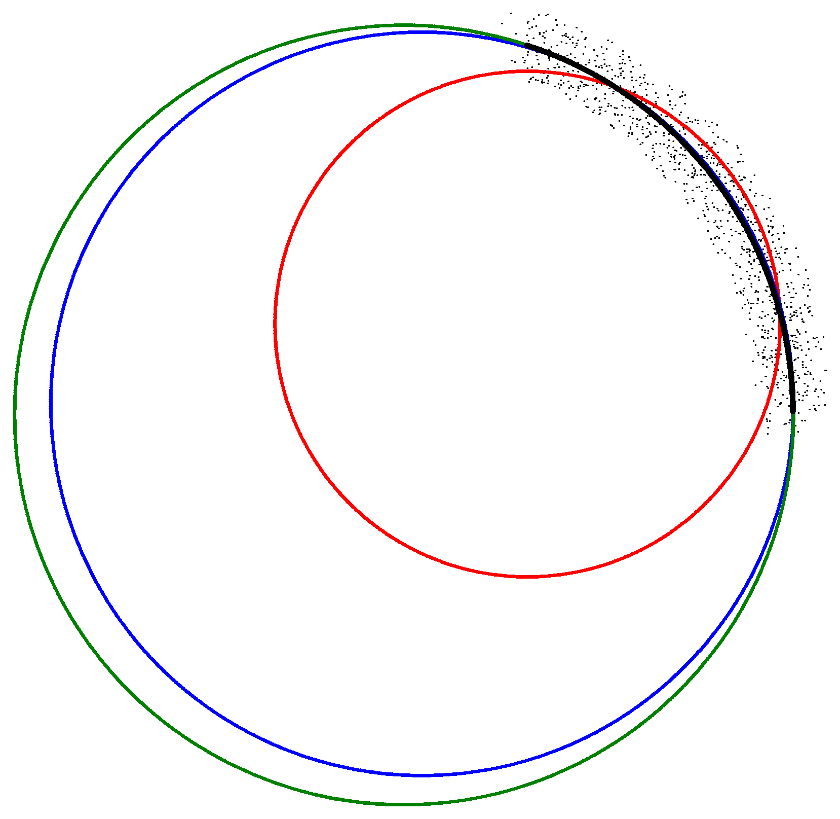
From this formula, it is clear that the fitting is trying to decrease the radius to minimize (1). When the points cover only a small part of a circle, the estimated center of the circle can move toward the arc to reduce the radius, see Fig. 1. However, the errors are increased, while the overall penalty (1) is decreased. The smaller the angle of the arc, the worse the effect.

Minimizing the next equation was suggested in [5]:

leading to the next error formula

This doesn’t encounter a problem like in (2). However, minimizing (3) requires an iterative approach, which analyzes all points $\displaystyle(x_{i},y_{i})$ leading to an algorithm with complexity $\displaystyle O{\left(n\right)}$. The efficient algorithm to find the minimum of (3) is described in [6].

The solution to remove the square root from (3) was developed in [7], [8, see p. 675], [9], and [1]. From (2) comes an idea that dividing (1) by $\displaystyle 4r^{2}$ and minimizing it will produce a result closer to (3) because it is close to (4). The approximation based on the Taylor expansion of the square root by the first two terms gives exactly this solution. Approximation of $\displaystyle\sqrt{x}$ at $\displaystyle x=1$:

Applying this approximation to (3)

Unlike (3), this formula can be minimized using only moments. The direct solution, based on conformal geometric algebra, is described in [1]. The solution is based on finding eigenvalues of a square nonsymmetric matrix [1, see (24)]. This can be done using Schur factorization. The eigenvector corresponding to the minimal non-negative eigenvalue is the solution. Care should be taken in cases where the solution has close to zero eigenvalue due to round-off error.

In this paper, another approach to minimization of (5) will be considered.

Starting from a good estimate $\displaystyle\left(x_{e},y_{e},r_{e}\right)$, the search for the optimum can be performed in the next form: $\displaystyle\left(x_{e}+\Delta{x},y_{e}+\Delta{y},\sqrt{r_{e}^{2}+\Delta{x^{2}}+\Delta{y^{2}}+\Delta{r}}\right).$

This covers all possible values of $\displaystyle\left(x_{c},y_{c},r\right)$ and gives the significant advantage for finding the minimum by removing the third and fourth order variables in the numerator of (5):

Writing it from moments

where

Minimization of (6) can be done using the approach described in Appendix II. To use that approach, it is sufficient to know the matrix of second derivatives up to the constant

where

and the equation for directional search by direction $\displaystyle\left(\alpha_{x},\alpha_{y},\alpha_{r}\right)$ is

Looking at the numerator of (5), it would be reasonable to take a solution of (1), described in [3], as a starting point.

Only a few iterations are needed to converge beyond machine precision. Because this approach is only an approximation, there is no need for such precision. In practice, one iteration is sufficient to get a good approximation.

When estimation of the center is known, the best estimation of the radius can be easily found. However, it does not give any improvement in speed.

An approximation of the sum of squared deviations from the polyline to an arc with the center $\displaystyle\left(x_{e},y_{e}\right)$ and radius $\displaystyle r_{e}$ (see (3)) is found from (6) by setting $\displaystyle\Delta{x}$, $\displaystyle\Delta{y}$, and $\displaystyle\Delta{r}$ to zero and multiplying by $\displaystyle n$.

The algorithm described in [1] has the advantage of finding the global optimum, while the algorithm described in this paper can find the local optimum. This is likely to happen when the arc is close to the line. Otherwise, the results are identical.

The advantage of the approach described in this paper is the ability to reduce the amount of calculation by approximating the solution.

I have implemented both approaches. Intel Math Kernel Library $\displaystyle 11.2$ was used to solve the nonsymmetric eigenvector problem in [1]. The approach described in this paper is several times faster. However, it is difficult to make a fair comparison due to the different ways of implementing and optimizing the code. When speed is not a concern, the approach described in [1] is preferred.

A comparison of fitting quality is done in Table 1. There are situations when fitting cannot be done for all or some approaches. To overcome this difficulty, the median is used. The number of points is $\displaystyle 1,000$. The number of simulations is $\displaystyle 1,000,001$. The ground truth circle has a radius of $\displaystyle 1$. The noise is uniform and perpendicular to the circumference of the circle.

Assuming that the center of the unit circle is known and the errors are distributed uniformly in $\displaystyle\left[-w,w\right]$, $\displaystyle 0\leq w\wedge w\leq 1$, perpendicular to the circumference of the unit circle, the bias is equal to

Therefore, the estimated radius tends to be larger than the true radius. For example, for the uniform noise of $\displaystyle 7$ percent, the error in the estimation of radius is less than $\displaystyle 0.1$ percent.

When enough information is available to reconstruct an arc, all approaches perform equally well. The approximation of the square root has minimum effect, unless the noise is large and the arc is small. When the arc is too small for the approach described in this paper, one iteration is definitely not enough. Note that in this case, the arc is very close to the line. The approach described in [6] sometimes fails because it might perform division by numbers close to zero; however, the arc can be reconstructed using other approaches. It is possible to improve the stability of convergence in [6] by providing a better starting point, for example, by the algorithm described in this paper, with a sufficient number of iterations.

The comparison of fitting speed is performed by averaging the time used by each approach for $\displaystyle 10,000$ simulations of the $\displaystyle 72\degree$ arc with uniform noise proportional to $\displaystyle 10$ percent of the arc radius. Points are simulated along the arc with uniform steps. When moments up to the fourth order are known, the described approach becomes faster at $\displaystyle 5$ points. The described approach has constant complexity, while the iterative approach has linear complexity. For $\displaystyle 100$ points, the advantage in speed is about $\displaystyle 9$ times. When moments have to be calculated, it is faster at $\displaystyle 6$ points. For $\displaystyle 100$ points, the advantage in speed is about $\displaystyle 3.5$ times.

For some tasks, one point on the arc is known in advance. The arc should pass through that point. Knowing the position of the center determines the radius: $\displaystyle r=\sqrt{\left(\left(x_{c}-x_{a}\right)^{2}+\left(y_{c}-y_{a}\right)^{2}\right)}$, where $\displaystyle\left(x_{a},y_{a}\right)$ is a point on the arc. Substituting this into (5)

The solution described in Sect. 3 can be applied. The differences are that the optimization is performed in two-dimensional space, and the initial solution can be found from the least squares approach.

Multiplying the numerator and denominator of (8) by $\displaystyle s^{2}$ and replacing $\displaystyle x_{c}\cdot s$ and $\displaystyle y_{c}\cdot s$ by $\displaystyle u_{x}$ and $\displaystyle u_{y}$, respectively, and setting $\displaystyle u={\begin{pmatrix}u_{x}&u_{y}&s\end{pmatrix}}^{\top}$

where

Equation (9) is a generalized Rayleigh quotient. Note that $\displaystyle A$ and $\displaystyle B$ are symmetric non-negative matrices. The solution can be found by the generalized singular value decomposition of $\displaystyle\sqrt{A}$ and $\displaystyle\sqrt{B}$. Square root matrices can be found from singular value decompositions such as

where $\displaystyle L_{A}$ and $\displaystyle L_{B}$ are eigenvalue matrices of $\displaystyle A$ and $\displaystyle B$, respectively; $\displaystyle X_{A}$ and $\displaystyle X_{B}$ are eigenvector matrices of $\displaystyle A$ and $\displaystyle B$, respectively.

From generalized singular value decomposition for $\displaystyle\sqrt{A}$ and $\displaystyle\sqrt{B}$ follows

where $\displaystyle U$, $\displaystyle V$, and $\displaystyle Q$ are orthogonal matrices; $\displaystyle R$ is an upper triangular matrix.

From (10) and (11) follows

The smallest ratio of squares of eigenvalues is the solution. The center of the arc is recovered from $\displaystyle u$ as $\displaystyle\left(\dfrac{u_{x}}{s},\dfrac{u_{y}}{s}\right)$.

There are tasks when the starting and ending points of the arc are known (or any two points lying on the arc). Therefore, the center of the arc should lie on some line of $\displaystyle\left(x_{c},y_{c}\right)=\left(x_{p}+\alpha\cdot t,y_{p}+\beta\cdot t\right)$, where $\displaystyle\left(x_{p},y_{p}\right)$ is a point on the line, $\displaystyle\left(\alpha,\beta\right)$ is the direction of the line ($\displaystyle\alpha^{2}+\beta^{2}=1$), and $\displaystyle t$ is any value. Knowing the position of the center determines the radius:

where $\displaystyle\left(x_{a},y_{a}\right)$ is one of the points on the arc. Substituting this in (5)

where

The minimum of (12) can be easily found because it has the form of (13) in Appendix I. An iterative algorithm is not needed to solve this problem.

The algorithm described in [2] finds an optimal polyline within the tolerance of the source polyline, with the minimum number of vertices, and among them, with the minimum sum of the squared deviations from the optimal polyline. Extending this algorithm to support arcs requires efficient fitting of the arc from the known start and end points and evaluation of the sum of the squared deviations from the source polyline to an arc. An approximate solution (7) can be used instead of direct evaluation (3).

The approach described in this paper for efficiently fitting circular arcs is used in a compression algorithm, when vertices of the source polylines are not allowed to move. The algorithm minimizes the weighted number of segments (with penalty 2) and arcs (with penalty 3) while satisfying tolerance restrictions. Among all possible solutions, the solution with the minimum sum of squared deviations is chosen. A dynamic programming approach was used to find the optimal solution, see [10], [11], [12], and [2].¹¹ 1 The penalty function in [12] is a combination of perceptual and fitting errors. The perceptual error is $\displaystyle\delta\cdot\sin{\dfrac{\alpha}{2}}$, where $\displaystyle\delta$ is the segmentation penalty and $\displaystyle\alpha$ is the angle between adjacent segments. This gives preference to solutions with acute angles.

Fitting of arcs in [10] was performed by checking tolerance when starting and ending vertices are fixed. It has the advantage of always finding an arc within tolerance; however, the computational complexity for each fitting is $\displaystyle O{\left(n\log{\left(n\right)}\right)}$. This paper uses approximation to least squares fitting with complexity $\displaystyle O{\left(1\right)}$ described in Sect. 6. Although checking for the tolerance and proper sequence (zigzag) ([10], [6], and [2]) has complexity $\displaystyle O{\left(n\right)}$, it is only performed for optimal fits.

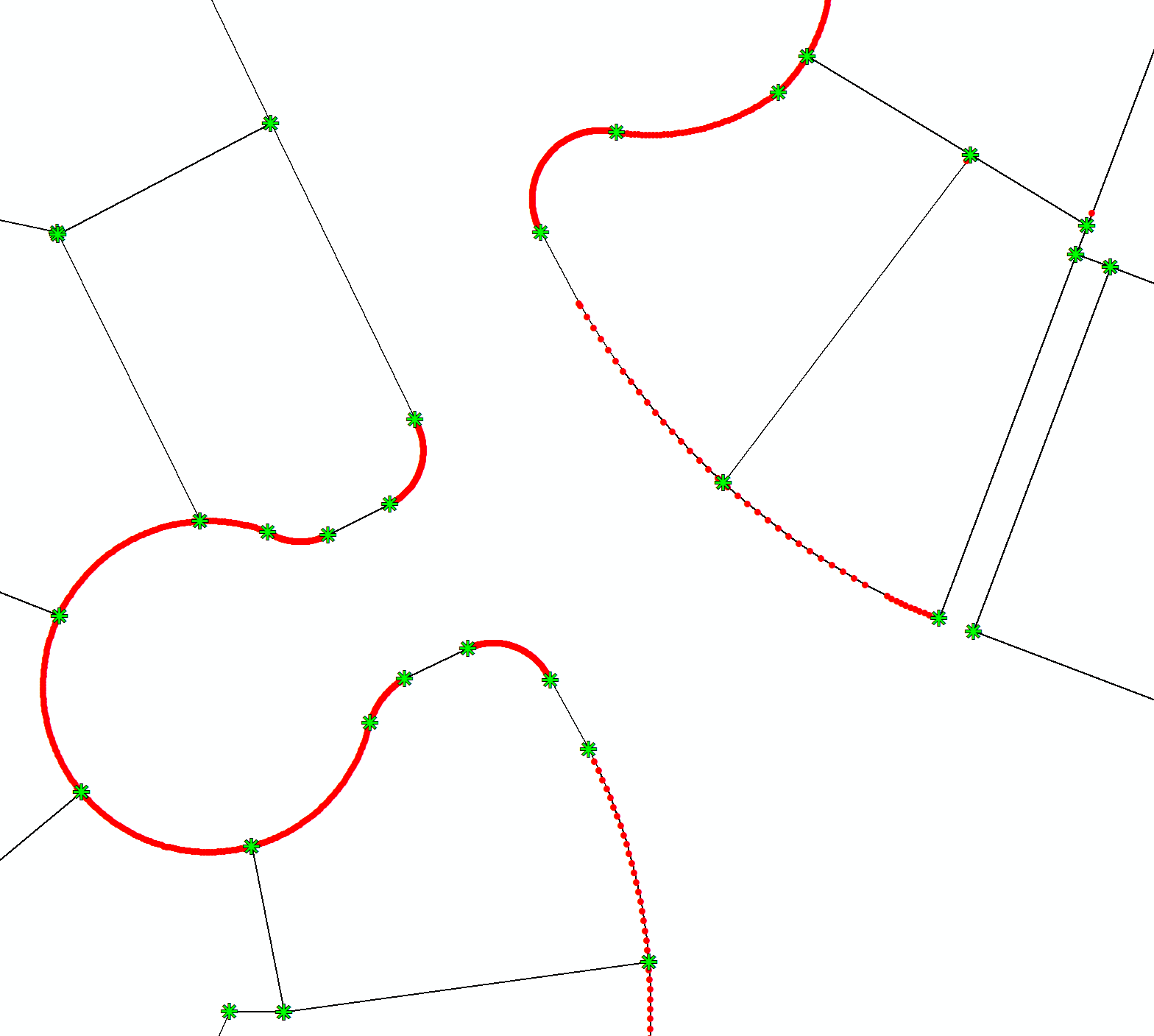
An example is shown in Fig. 2. The original arcs were lost due to digitization, limitations of the format, projection, and so forth. The restoration of arcs is an important task because restoring original arcs creates cleaner databases and simplifies future editing.

This paper describes an efficient method of approximate fitting circular arcs. While all formulas are for a two-dimensional case, the algorithm can be generalized for higher dimensions (for example, fitting a sphere to points).

The direct solution to fit arcs is described in [1]. This paper extends the solution to cases when one or two points on the arc are known.

Because the solution is based on fourth orders, it has a negative impact on the precision of calculations. This can be solved by shifting data to the origin of a coordinate system and/or using floating point numbers with a larger mantissa. Another solution is to place points into an integer coordinate system and calculate all moments using exact arithmetic on integer numbers. Than for fitting an arc to a subset of points, recalculate moments for the origin closer to the center of an arc.

There is no evaluation of how well the fit is done. An additional algorithm is necessary to perform this check, as described in [6, see Sect. 3].

The author would like to thank Linda Thomas, Lois Stuart, and Mary Anne Chan for proofreading this paper.

References

- [1] L. Dorst, “Total least squares fitting of k-spheres in n-d Euclidean space using an (n+2)-d isometric representation,” Journal of Mathematical Imaging and Vision, vol. 50, no. 3, pp. 214–234, 2014. [Online]. Available: http://doi.org/10.1007/s10851-014-0495-2
- [2] A. Gribov, “Searching for a compressed polyline with a minimum number of vertices,” in 2017 14th IAPR International Conference on Document Analysis and Recognition (ICDAR), vol. 02, November 2017, pp. 13–14. [Online]. Available: http://doi.org/10.1109/ICDAR.2017.254
- [3] S. M. Thomas and Y. T. Chan, “A simple approach for the estimation of circular arc center and its radius,” Computer Vision, Graphics, and Image Processing, vol. 45, no. 3, pp. 362–370, March 1989. [Online]. Available: http://doi.org/10.1016/0734-189X(89)90088-1
- [4] C. Ichoku, B. Deffontaines, and J. Chorowicz, “Segmentation of digital plane curves: A dynamic focusing approach,” Pattern Recognition Letters, vol. 17, no. 7, pp. 741–750, June 1996. [Online]. Available: http://doi.org/10.1016/0167-8655(96)00015-3
- [5] S. M. Robinson, “Fitting spheres by the method of least squares,” Communications of the ACM, vol. 4, no. 11, p. 491, November 1961. [Online]. Available: http://doi.org/10.1145/366813.366824
- [6] E. Bodansky and A. Gribov, “Approximation of polylines with circular arcs,” in Graphics Recognition. Recent Advances and Perspectives, ser. Lecture Notes in Computer Science, J. Lladós and Y.-B. Kwon, Eds. Springer Berlin Heidelberg, 2004, vol. 3088, pp. 193–198. [Online]. Available: http://doi.org/10.1007/978-3-540-25977-0_18
- [7] V. Pratt, “Direct least-squares fitting of algebraic surfaces,” SIGGRAPH ’87 Proceedings of the 14th annual conference on Computer graphics and interactive techniques, vol. 21, no. 4, pp. 145–152, Aug. 1987. [Online]. Available: http://doi.org/10.1145/37402.37420
- [8] G. Lukács, R. Martin, and D. Marshall, “Faithful least-squares fitting of spheres, cylinders, cones and tori for reliable segmentation,” in Computer Vision - ECCV’98, ser. Lecture Notes in Computer Science, H. Burkhardt and B. Neumann, Eds. Springer Berlin Heidelberg, 1998, vol. 1406, pp. 671–686. [Online]. Available: http://doi.org/10.1007/BFb0055697
- [9] A. Fitzgibbon, M. Pilu, and R. B. Fisher, “Direct least square fitting of ellipses,” IEEE Transactions on Pattern Analysis and Machine Intelligence, vol. 21, no. 5, pp. 476–480, May 1999. [Online]. Available: http://doi.org/10.1109/34.765658
- [10] A. Safonova and J. Rossignac, “Compressed piecewise-circular approximations of 3D curves,” Computer-Aided Design, vol. 35, pp. 533–547, May 2003. [Online]. Available: http://doi.org/10.1016/S0010-4485(02)00073-8
- [11] A. Gribov and E. Bodansky, “A new method of polyline approximation,” in Structural, Syntactic, and Statistical Pattern Recognition, ser. Lecture Notes in Computer Science, A. Fred, T. M. Caelli, R. P. Duin, A. Campilho, and D. de Ridder, Eds. Springer Berlin Heidelberg, 2004, vol. 3138, pp. 504–511. [Online]. Available: http://doi.org/10.1007/978-3-540-27868-9_54
- [12] L. Yin, Y. Yajie, and L. Wenyin, “Online segmentation of freehand stroke by dynamic programming,” in Eighth International Conference on Document Analysis and Recognition, vol. 1, August 2005, pp. 197–201. [Online]. Available: http://doi.org/10.1109/ICDAR.2005.180