Double parton scattering at high energies Thanks: Presented at the XXI Cracow EPIPHANY Conference on Future High Energy Colliders

Let us consider first production of $c\bar{c}c\bar{c}$ final state within the DPS framework. In a simple probabilistic picture the cross section for double-parton scattering can be written as:

$$\sigma^{DPS}(pp\to c\bar{c}c\bar{c}X)=\frac{1}{2\sigma_{eff}}\sigma^{SPS}(pp\to c\bar{c}X_{1})\cdot\sigma^{SPS}(pp\to c\bar{c}X_{2}).$$

(1)

This formula assumes that the two subprocesses are not correlated. At low energies one has to include parton momentum conservation i.e. extra limitations: $x_{1}+x_{3}<$ 1 and $x_{2}+x_{4}<$ 1, where $x_{1}$ and $x_{3}$ are longitudinal momentum fractions of gluons emitted from one proton and $x_{2}$ and $x_{4}$ their counterpairs for gluons emitted from the second proton. Experimental data [55] provide an estimate of $\sigma_{eff}$ in the denominator of formula (1). In our studies presented here we usually take $\sigma_{eff}$ = 15 mb.

The simple formula (1) can be generalized to address differential distributions. In leading-order approximation differential distribution can be written as

$$\frac{d\sigma}{dy_{1}dy_{2}d^{2}p_{1t}dy_{3}dy_{4}d^{2}p_{2t}}\\ =\frac{1}{2\sigma_{eff}}\frac{d\sigma}{dy_{1}dy_{2}d^{2}p_{1t}}\cdot\frac{d\sigma}{dy_{3}dy_{4}d^{2}p_{2t}}$$

(2)

which by construction reproduces formula for integrated cross section (1). This cross section is formally differential in 8 dimensions but can be easily reduced to 7 dimensions noting that physics of unpolarized scattering cannot depend on azimuthal angle of the pair or on azimuthal angle of one of the produced $c$ ($\bar{c}$) quark (antiquark). The differential distributions for each single scattering step can be written in terms of collinear gluon distributions with longitudinal momentum fractions $x_{1}$, $x_{2}$, $x_{3}$ and $x_{4}$ expressed in terms of rapidities $y_{1}$, $y_{2}$, $y_{3}$, $y_{4}$ and transverse momenta of quark (or antiquark) for each step (in the LO approximation identical for quark and antiquark).

A more general formula for the cross section can be written formally in terms of double-parton distributions, e.g. $F_{gg}$, $F_{qq}$, etc. In the case of heavy quark (antiquark) production at high energies:

	$\displaystyle d\sigma^{DPS}$	$\displaystyle=$	$\displaystyle\frac{1}{2\sigma_{eff}}F_{gg}(x_{1},x_{2},\mu_{1}^{2},\mu_{2}^{2})F_{gg}(x^{\prime}_{1}x^{\prime}_{2},\mu_{1}^{2},\mu_{2}^{2})$		(3)
			$\displaystyle d\sigma_{gg\to c\bar{c}}(x_{1},x^{\prime}_{1},\mu_{1}^{2})d\sigma_{gg\to c\bar{c}}(x_{2},x^{\prime}_{2},\mu_{2}^{2})\;dx_{1}dx_{2}dx^{\prime}_{1}dx^{\prime}_{2}\,.$

It is rather inspiring to write the double-parton distributions in the impact parameter space $F_{gg}(x_{1},x_{2},b)=g(x_{1})g(x_{2})F(b)$, where $g$ are usual conventional parton distributions and $F(b)$ is an overlap of the matter distribution in the transverse plane where $b$ is a distance between both gluons in the transverse plane [56]. The effective cross section in (1) is then $1/\sigma_{eff}=\int d^{2}bF^{2}(b)$ and in this approximation is energy independent.

Even if the factorization is valid at some scale, QCD evolution may lead to a factorization breaking. Evolution is known only in the case when the scale of both scatterings is the same [19, 20, 22] i.e. for heavy object, like double gauge boson production.

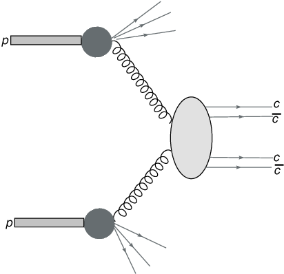
In Ref. [27] we applied the commonly used in the literature factorized model to $pp\to c\bar{c}c\bar{c}$ and predicted that at the LHC energies the cross section for two $c\bar{c}$ pair production starts to be of the same size as that for single $c\bar{c}$ production.

In LO collinear approximation the differential distributions for $c\bar{c}$ production depend e.g. on rapidity of quark, rapidity of antiquark and transverse momentum of one of them [27]. In the next-to-leading order (NLO) collinear approach or in the $k_{t}$-factorization approach the situation is more complicated as there are more kinematical variables needed to describe the kinematical situation. In the $k_{t}$-factorization approach the differential cross section for DPS production of $c\bar{c}c\bar{c}$ system, assuming factorization of the DPS model, can be written as:

	$\displaystyle\frac{d\sigma^{DPS}(pp\to c\bar{c}c\bar{c}X)}{dy_{1}dy_{2}d^{2}p_{1,t}d^{2}p_{2,t}dy_{3}dy_{4}d^{2}p_{3,t}d^{2}p_{4,t}}=\;\;\;\;\;\;\;\;\;\;\;\;\;\;\;\;\;\;\;\;\;\;\;\;\;\;\;\;\;\;\;\;\;\;\;\;\;\;\;\;\;\;\;\;$
	$\displaystyle\frac{1}{2\sigma_{eff}}\cdot\frac{d\sigma^{SPS}(pp\to c\bar{c}X_{1})}{dy_{1}dy_{2}d^{2}p_{1,t}d^{2}p_{2,t}}\cdot\frac{d\sigma^{SPS}(pp\to c\bar{c}X_{2})}{dy_{3}dy_{4}d^{2}p_{3,t}d^{2}p_{4,t}}.$		(4)

Again when integrating over kinematical variables one recovers Eq.(1).

$$\sigma_{eff}=\left[\int d^{2}b\;(T(\vec{b}))^{2}\right]^{-1},$$

(5)

where the overlap function

$$T(\vec{b})=\int f(\vec{b}_{1})f(\vec{b}_{1}-\vec{b})\;d^{2}b_{1},$$

(6)

if the impact-parameter dependent double-parton distributions (dPDFs) are written in the following factorized approximation [22, 57]:

$$\Gamma_{i,j}(x_{1},x_{2};\vec{b}_{1},\vec{b}_{2};\mu_{1}^{2},\mu_{2}^{2})=F_{i,j}(x_{1},x_{2};\mu_{1}^{2},\mu_{2}^{2})\;f(\vec{b}_{1})\;f(\vec{b}_{2}).$$

(7)

Without loosing generality the impact-parameter distribution can be written as

$$\Gamma(b,x_{1},x_{2};\mu_{1}^{2},\mu_{2}^{2})=F(x_{1},\mu_{1}^{2})\;F(x_{2},\mu_{2}^{2})\;F(b;x_{1},x_{2},\mu_{1}^{2},\mu_{2}^{2}),\;$$

(8)

where $b$ is the parton separation in the impact parameters space. In the formula above the function $F(b;x_{1},x_{2},\mu_{1}^{2},\mu_{2}^{2})$ contains all information about correlations between the two partons (two gluons in our case). The dependence was studied numerically in Ref. [57] within Lund Dipole Cascade model. The biggest discrepancy was found in the small $b$ region, particularly for large $\mu_{1}^{2}$ and/or $\mu_{2}^{2}$. We shall return to the issue when commenting our results. In general the effective cross section may depend on many kinematical variables:

$$\sigma_{eff}(x_{1},x_{2},x^{\prime}_{1},x^{\prime}_{2},\mu_{1}^{2},\mu_{2}^{2})=\left(\int d^{2}b\;F(b;x_{1},x_{2},\mu_{1}^{2},\mu_{2}^{2})\;F(b;x^{\prime}_{1},x^{\prime}_{2},\mu_{1}^{2},\mu_{2}^{2})\right)^{-1}.$$

(9)

We shall return to these dependences when discussing the role of perturbative parton splitting.

In Fig. 4 we illustrate a conventional and perturbative DPS mechanisms for $c\bar{c}c\bar{c}$ production. The 2v1 mechanism (the second and third diagrams) were considered first in [58].

In the case of $c\bar{c}c\bar{c}$ production the cross section for conventional DPS can be written as:

	$\displaystyle\sigma(2v2)$	$\displaystyle=$	$\displaystyle\frac{1}{2}\frac{1}{\sigma_{eff,2v2}}\int dy_{1}dy_{2}d^{2}p_{1t}dy_{3}dy_{4}d^{2}p_{2t}\frac{1}{16\pi{\hat{s}}^{2}}\overline{|{\cal M}(gg\to c\bar{c})|^{2}}\;x_{1}x_{1}^{\prime}x_{2}x_{2}^{\prime}$		(10)
			$\displaystyle\times\;D^{gg}(x_{1},x_{2},\mu_{1}^{2},\mu_{2}^{2})\;D^{gg}(x_{1},x_{2},\mu_{1}^{2},\mu_{2}^{2})$

while that for the perturbative parton splitting DPS in a very similar fashsion (see e.g.[58])

	$\displaystyle\sigma(2v1)$	$\displaystyle=$	$\displaystyle\frac{1}{2}\frac{1}{\sigma_{eff,2v1}}\int dy_{1}dy_{2}d^{2}p_{1t}dy_{3}dy_{4}d^{2}p_{2t}\frac{1}{16\pi{\hat{s}}^{2}}\overline{|{\cal M}(gg\to c\bar{c})|^{2}}\;x_{1}x_{1}^{\prime}x_{2}x_{2}^{\prime}$
			$\displaystyle\!\!\!\!\!\!\!\!\!\!\!\!\!\!\!\!\!\!\!\!\!\!\!\!\!\!\!\!\!\!\!\times\;\left({\hat{D}}^{gg}(x_{1}^{\prime},x_{2}^{\prime},\mu_{1}^{2},\mu_{2}^{2})D^{gg}(x_{1},x_{2},\mu_{1}^{2},\mu_{2}^{2})+\;D^{gg}(x_{1}^{\prime},x_{2}^{\prime},\mu_{1}^{2},\mu_{2}^{2}){\hat{D}}^{gg}(x_{1},x_{2},\mu_{1}^{2},\mu_{2}^{2})\right)$

In the calculations performed in Ref. [59] all partonic cross sections are calculated only in leading order. The cross section for dijet production can be written then as:

$$\frac{d\sigma(ij\to kl)}{dy_{1}dy_{2}d^{2}p_{t}}=\frac{1}{16\pi^{2}{\hat{s}}^{2}}\sum_{i,j}x_{1}f_{i}(x_{1},\mu^{2})\;x_{2}f_{j}(x_{2},\mu^{2})\;\overline{|\mathcal{M}_{ij\to kl}|^{2}}\;,$$

(12)

where $y_{1}$, $y_{2}$ are rapidities of the two jets and $p_{t}$ is transverse momentum of one of them (identical).

In our calculations we include all leading-order $ij\to kl$ partonic subprocesses (see e.g. [60, 61]). The $K$-factor for dijet production is rather small, of the order of $1.1-1.3$ (see e.g. [62, 63]), and can be easily incorporated in our calculations. Below we shall show that already the leading-order approach gives results in reasonable agreement with recent ATLAS [64] and CMS [65] data.

This simplified leading-order approach was used in our first estimate of DPS differential cross sections for jets widely separated in rapidity [59]. Similarly as for $c\bar{c}c\bar{c}$ production one can write:

	$\displaystyle\frac{d\sigma^{DPS}(pp\to\textrm{4jets}\;X)}{dy_{1}dy_{2}d^{2}p_{1t}dy_{3}dy_{4}d^{2}p_{2t}}$	$\displaystyle=$			(13)
			$\displaystyle\!\!\!\!\!\!\!\!\!\!\!\!\!\!\!\!\!\!\!\!\!\!\!\!\!\!\!\!\!\!\!\!\!\!\!\!\!\!\!\!\!\!\!\!\!\!\!\!\!\!\!\!\!\!\!\!\sum\nolimits_{i_{1},j_{1},k_{1},l_{1},i_{2},j_{2},k_{2},l_{2}}\;\frac{\mathcal{C}}{\sigma_{eff}}\;\frac{d\sigma(i_{1}j_{1}\to k_{1}l_{1})}{dy_{1}dy_{2}d^{2}p_{1t}}\;\frac{d\sigma(i_{2}j_{2}\to k_{2}l_{2})}{dy_{3}dy_{4}d^{2}p_{2t}}\;,$

where $\mathcal{C}=\left\{\begin{array}[]{ll}\frac{1}{2}&\textrm{if}\;\;i_{1}j_{1}=i_{2}j_{2}\wedge k_{1}l_{1}=k_{2}l_{2}\\ 1&\textrm{if}\;\;i_{1}j_{1}\neq i_{2}j_{2}\vee k_{1}l_{1}\neq k_{2}l_{2}\end{array}\right\}$ and partons $j,k,l,m=g,u,d,s,\bar{u},\bar{d},\bar{s}$. The combinatorial factors include identity of the two subprocesses. Each step of the DPS is calculated in the leading-order approach (see Eq.(12)). Above $y_{1}$, $y_{2}$ and $y_{3}$, $y_{4}$ are rapidities of partons in first and second partonic subprocess, respectively. The $p_{1t}$ and $p_{2t}$ are respective transverse momenta.

Experimental data from the Tevatron [55] and the LHC [66, 28, 67] provide an estimate of $\sigma_{eff}$ in the denominator of formula (13). As in our recent paper [68] we take $\sigma_{eff}$ = 15 mb. A detailed analysis of $\sigma_{eff}$ based on various experimental data can be found in Refs. [69, 70].

The diagram representating the double parton scattering process is shown in Fig. 5. The cross section for double parton scattering is often modelled in the factorized anzatz which in our case would mean:

$$\sigma_{W^{+}W^{-}}^{DPS}=\frac{1}{\sigma_{qq}^{eff}}\sigma_{W^{+}}\sigma_{W^{-}}\;.$$

(14)

In general, the parameter $\sigma_{qq}$ does not need to be the same as for gluon-gluon initiated processes $\sigma_{gg}^{eff}$. In the present, rather conservative, calculations we take it to be $\sigma_{qq}^{eff}=\sigma_{gg}^{eff}$ = 15 mb. The latter value is known within about 10 % from systematics of gluon-gluon initiated processes at the Tevatron and LHC.

The factorized model (14) can be generalized to more differential distributions. For example in our case of $W^{+}W^{-}$ production the cross section differential in $W$ boson rapidities can be written as:

$$\frac{d\sigma_{W^{+}W^{-}}^{DPS}}{dy_{+}dy_{-}}=\frac{1}{\sigma_{qq}^{eff}}\frac{d\sigma_{W}^{+}}{dy_{+}}\frac{d\sigma_{W}^{-}}{dy_{-}}\;.$$

(15)

In particular, in leading-order approximation the cross section for quark-antiquark annihilation reads:

	$\displaystyle\frac{d\sigma}{dy}$	$\displaystyle=$	$\displaystyle\sum_{ij}\left(x_{1}q_{i/1}(x_{1},\mu^{2})x_{2}{\bar{q}}_{j/2}(x_{2},\mu^{2})+x_{1}{\bar{q}}_{i/1}(x_{1},\mu^{2})x_{2}q_{j/2}(x_{1},\mu^{2})\right)$		(16)
			$\displaystyle\;\times\;\overline{|{\cal M}_{ij\to W^{\pm}}|^{2}}$

where the matrix element for quark-antiquark annihilation to $W$ bosons (${\cal M}_{ij\to W^{\pm}}$) contains Cabibbo-Kobayashi-Maskawa matrix elements.

When calculating the cross section for single $W$ boson production in leading-order approximation a well known Drell-Yan $K$-factor can be included. The double-parton scattering would be then multiplied by $K^{2}$.

We start presentation of our results with production of two pairs of $c\bar{c}$. In Fig. 6 we compare cross sections for the single and double-parton scattering as a function of proton-proton center-of-mass energy. At low energies the single-parton scattering dominates. For reference we show the proton-proton total cross section as a function of collision energy as parametrized in Ref. [71]. At low energy the $c\bar{c}$ or $c\bar{c}c\bar{c}$ cross sections are much smaller than the total cross section. At higher energies both the contributions dangerously approach the expected total cross section. This shows that inclusion of unitarity effect and/or saturation of parton distributions may be necessary. The effects of saturation in $c\bar{c}$ production were included e.g. in Ref. [72] but not checked versus experimental data. Presence of double-parton scattering changes the situation. The double-parton scattering is potentially very important ingredient in the context of high energy neutrino production in the atmosphere [73, 74, 72] or of cosmogenic origin [75]. At LHC energies the cross section for both terms become comparable. This is a completely new situation.

So far we have concentrated on DPS production of $c\bar{c}c\bar{c}$ and completely ignored SPS production of $c\bar{c}c\bar{c}$. In Refs.[76, 68] we calculated the SPS contribution in high-energy approximation [76] and including all diagrams in the collinear-factorization approach [68]. In Fig. 7 we show the cross section from Ref. [68]. The corresponding cross section at the LHC energies is more than two orders of magnitude smaller than that for $c\bar{c}$ production i.e. much smaller than the DPS contribution discussed in the previous figure.

In experiment one measures $D$ mesons instead of charm quarks/antiquarks. In Fig. 8 we show resulting distributions in rapidity distance between two $D^{0}$ mesons (left panel) and corresponding distribution in relative azimuthal angle (right panel). The DPS contribuion (dashed line) dominates over the single parton scattering one (dash-dotted line). The sum of the two contributions is represented by the solid line. We get a reasonable agreement with the LHCb experimental data [28].

Distribution in the invariant mass of two $D^{0}D^{0}$ mesons is shown in Fig. 9. Again a reasonable agreement is obtained. Some strength is missing in the interval 10 GeV $<M_{D^{0}D^{0}}<$ 16 GeV.

At the LHC the cross section for $pp\to c\bar{c}$ is still bigger than that for $pp\to c\bar{c}c\bar{c}$ [29]. As shown in Fig. 6 the latter cross section is growing fast and at high energy it may become even larger than that for single pair production. The situation at Future Circular Collider (FCC) is shown in Fig. 10. Now the situation reverses and the cross section for $c\bar{c}c\bar{c}$ is bigger than that for single pair production. We predict rather flat distributions in charm quark/antiquark rapidities. The shapes in quark/aniquark transverse momenta are almost identical which can be easily understood within the formalism presented in the previous section.

As described in the Formalism section the splitting contributions are calculated in leading order only. In the calculations performed in Ref. [58] we either assumed $\mu_{1}^{2}=m_{1t}^{2}$ and $\mu_{2}^{2}=m_{2t}^{2}$, or $\mu_{1}^{2}=M_{c\bar{c},1}^{2}$ and $\mu_{2}^{2}=M_{c\bar{c},2}^{2}$. The quantity $m_{it}$ is the transverse mass of either parton emerging from subprocess $i$, whilst $M_{c\bar{c},i}$ is the invariant mass of the pair emerging from subprocess $i$.

In Fig. 11 we show the rapidity distribution of the charm quark/antiquark for different choices of the scale at $\sqrt{s}$ = 7 TeV. The conventional and splitting terms are shown separately. The splitting contribution (lowest curve, red online) is smaller, but has almost the same shape as the conventional DPS contribution. We can observe asymmetric (in rapidity) shapes for the $1v2$ and $2v1$ contributions.

The corresponding ratios of the 2v1-to-2v2 contributions as a function of rapidity is shown in Fig. 12.

In Fig. 13 we show energy deprendence of the ratio of the 2v1 to 2v2 cross sections. The ratio systematically decreases with the collision energy.

Finally in Fig. 14 we show the empirical $\sigma_{eff}$, for double charm production. Again $\sigma_{eff}$ rises with the centre-of-mass energy. A sizeable difference of results for different choices of scales can be observed.

In Fig. 15 we compare our calculation for inclusive jet production with the CMS data [65]. In addition, we show contributions of different partonic mechanisms. In all rapidity intervals the gluon-gluon and quark-gluon (gluon-quark) contributions clearly dominate over the other contributions and in practice it is sufficient to include only these subprocesses in further analysis.

Now we proceed to the jets with large rapidity separation. In Fig. 16 we show distribution in the rapidity distance between two jets in leading-order collinear calculation and between the most distant jets in rapidity in the case of four DPS jets. In this calculation we have included cuts for the CMS expriment [49]: $y_{1},y_{2}\in$ (-4.7,4.7), $p_{1t},p_{2t}\in$ (35 GeV, 60 GeV). For comparison we show also results for the BFKL calculation from Ref. [44]. For this kinematics the DPS jets give sizeable contribution only at large rapidity distance. The NLL BFKL cross section (long-dashed line) is smaller than that for the LO collinear approach (short-dashed line).

In Fig. 17 we show rapidity-distance distribution for even smaller lowest transverse momenta of the ”jet”. A measurement of such minijets may be, however, difficult. Now the DPS contribution may even exceed the standard SPS dijet contribution, especially at the nominal LHC energy. How to measure such (mini)jets is an open issue. In principle, one could measure correlations of semihard ($p_{t}\sim$ 10 GeV) neutral pions with the help of so-called zero-degree calorimeters (ZDC) which are installed by all major LHC experiments.

It was argued that the DPS contribution for inclusive $W^{+}W^{-}$ could be large [54]. Here we partly report results from Ref. [52]. In this analysis we have assumed $\sigma_{eff}$ = 15 mb as is a phenomenological standard for many other, mostly gluon-gluon induced, processes. Similar value was used also in other recent analysis [53] where in addition evolution effects of dPDFs were discussed. In our opinion the normalization of the cross section may be an open issue [52]. Therefore below we wish to compare rather shapes of a few distributions. In Fig. 18 we show two-dimensional distributions in rapidity of $W^{+}$ and $W^{-}$. For reference we show also distributions for $\gamma\gamma$ and $q\bar{q}$ components (see a detailed discussion in Ref. [52]). The DPS contribution seems broader in the $(y_{W^{+}},y_{W^{-}})$ space than the other two contributions.

In Fig. 19 we show invariant $M_{WW}$ mass distribution for $\sqrt{s}$ = 8 TeV. The DPS contribution seems to dominate at very large invariant masses.

How the situation may look at future high-energy experiments at the LHC and FCC is shown in Table 1 and Fig. 20. Now the DPS (conservative estimation) is relatively larger compared to other contributions.

In experiments one can measure charged leptons and not $W^{\pm}$ bosons. Therefore a detailed study of lepton distributions is needed. As en example we show (see Fig. 21) distribution of invariant mass of charged leptons compared with that for gauge bosons. Only a relatively small shift towards smaller invariant masses is observed. A more detailed studies are necessary to answer whether the $W^{+}W^{-}$ distribution can be identified experimentally. Several background contributions have to be considered. We leave such a detailed studies for future.

References

- [1] P.V. Landshoff and J.C. Polinghorne, Phys. Rev. D18 (1978) 3344.
- [2] F. Takagi, Phys. Rev. Lett. 18 (1979) 1296.
- [3] C. Goebel and D.M. Scott and F. Halzen, Phys. Rev. D22 (1980) 2789.
- [4] B. Humpert, Phys. Lett. B131 (1983) 461.
- [5] N. Paver and D. Treleani, Phys. Lett. B146 (1984) 252.
- [6] N. Paver and D. Treleani, Z. Phys. C28 (1985) 187.
- [7] M. Mekhfi, Phys. Rev. D32 2371; M. Mekhfi, Phys. Rev. D32 2380.
- [8] B. Humpert and R. Oderico, Phys. Lett. B154 (1985) 211.
- [9] T. Sjöstrand and M. van Zijl, Phys. Rev. D36 (1987) 2019.
- [10] M. Drees and T. Han, Phys. Rev. Lett. 77 (1996) 4142.
- [11] A. Kulesza and W.J. Stirling, Phys. Lett. B475 (2000) 168.
- [12] A. Del Fabbro and D. Treleani, Phys. Rev. D66 (2002) 074012.
- [13] E.L. Berger, C.B. Jackson and G. Shaughnessy, Phys. Rev. D81 014014 (2010).
- [14] J.R. Gaunt, C-H. Kom, A. Kulesza and W.J. Stirling, arXiv:1003.3953.
- [15] M. Strikman and W. Vogelsang, Phys. Rev. D83 (2011) 034029.
- [16] B. Blok, Yu. Dokshitzer, L. Frankfurt and M. Strikman, Phys. Rev. D83 (2011) 071501.
- [17] C.H. Khom, A. Kulesza and W.J. Stirling, Phys. Rev. Lett. 107 (2011) 082002.
- [18] S.R. Baranov, A. M. Snigirev and N.P. Zotov, arXiv:1105.6279.
- [19] A.M. Snigirev, Phys. Rev. D68 (2003) 114012.
- [20] V.L. Korotkikh and A.M. Snigirev, Phys. Lett. B594 (2004) 171.
- [21] T. Sjöstrand and P.Z. Skands, JHEP 0403 (2004) 053.
- [22] J.R. Gaunt and W.J. Stirling, JHEP 1003 (2010) 005.
- [23] J.R. Gaunt and W.J. Stirling, JHEP 1106 (2011) 048.
- [24] M. Diehl and A. Schäfer, Phys. Lett. B698 (2011) 389.
- [25] M.G. Ryskin and A.M. Snigirev, Phys. Rev. D83 (2011) 114047.
- [26] M. Diehl, D. Ostermeier and A. Schäfer, arXiv:1111.0910.
- [27] M. Łuszczak, R. Maciuła and A. Szczurek, Phys. Rev. D85 (2012) 094034.
- [28] R. Aaij et al. [LHCb Collaboration], J. High Energy Phys. 06, 141 (2012); J. High Energy Phys 03, 108 (2014); [arXiv:1205.0975 [hep-ex]].
- [29] R. Maciuła and A. Szczurek, Phys. Rev. D87 (2013) 074039.
- [30] A.V. Berezhnoy et al., Phys. Rev. D86 (2012) 034017.
- [31] A. H. Mueller, and H. Navelet, Nucl. Phys. B282, 727 (1987).
- [32] V. Del Duca and C. R. Schmidt, Phys. Rev. D49, 4510 (1994); arXiv:9311290 [hep-ph].
- [33] W. J. Stirling, Nucl. Phys. B423, 56 (1994); arXiv:9401266 [hep-ph].
- [34] V. Del Duca and C. R. Schmidt, Phys. Rev. D51, 2150 (1995); arXiv:9407359 [hep-ph].
- [35] V. T. Kim and G. B. Pivovarov, Phys. Rev. D 53, 6 (1996); arXiv:9506381 [hep-ph].
- [36] J. Andersen, V. Del Duca, S. Frixione, C. Schmidt and W. J Stirling, J. High Energy Phys. 02, 007 (2001); arXiv:0101180 [hep-ph].
- [37] J. Bartels, D. Colferai and G. Vacca, Eur. Phys. J. C24, 83 (2002); Eur. Phys. J. C 29, 235 (2003).
- [38] A. Sabio Vera and F. Schwennsen, Nucl. Phys. B776, 170 (2007); arXiv:0702158 [hep-ph].
- [39] C. Marquet and C. Royon, Phys. Rev. D79, 034028 (2009); arXiv:0704.3409 [hep-ph].
- [40] D. Colferai, F. Schwennsen, L. Szymanowski and S. Wallon, J. High Energy Phys. 12, 026 (2010); arXiv:1002.1365 [hep-ph].
- [41] F. Caporale, D. Y. Ivanov, B. Murdaca, A. Papa and A. Perri, J. High Energy Phys. 02, 101 (2012); arXiv:1112.3752 [hep-ph].
- [42] D. Y. Ivanov and A. Papa, J. High Energy Phys. 05, 086 (2012); arXiv:1202.1082 [hep-ph].
- [43] F. Caporale, D. Y. Ivanov, B. Murdaca and A. Papa, Nucl. Phys. B877, 73 (2013); arXiv:1211.7225 [hep-ph].
- [44] B. Ducloue, L. Szymanowski and S. Wallon, J. High Energy Phys. 05, 096 (2013); arXiv:1302.7012 [hep-ph].
- [45] B. Ducloué, L. Szymanowski and S. Wallon, Phys. Rev. Lett. 112, 082003 (2014); arXiv:1309.3229 [hep-ph].
- [46] V. Del Duca, L. J. Dixon, C. Duhr, J. Pennington, J. High Energy Phys. 02, 086 (2014): arXiv:1309.6647.
- [47] S. Chatrchyan et al. (the CMS Collaboration), CMS-PAS-FSQ-12-002 (2013).
- [48] P. Aurenche, R. Basu and M. Fontannaz, Eur. Phys. J. C57, 681 (2008); arXiv:0807.2133 [hep-ph].
- [49] I. Pozdnyakov, private communication
- [50] J.R. Gaunt, Ch.-H. Kom, A. Kulesza and W.J. Stirling, Eur. Phys. J. C69 (2010) 53, arXiv:1003.3953 [hep-ph].
- [51] J.R. Gaunt, Ch.-H. Kom, A. Kulesza and W.J. Stirling, arXiv:1110.1174 [hep-ph].
- [52] M. Luszczak, A. Szczurek and C. Royon, J. High Energy Phys. 02, 098 (2015); [arXiv:1409.1803 [hep-ph]].
- [53] K. Golec-Biernat and E. Lewandowska, Phys. Rev. D90 (2014) 094032.
- [54] W. Krasny and W. Płaczek, Acta Phys. Pol. B45 (2014) 71, arXiV:1305.1769 [hep-ph].
- [55]
F. Abe et al. (CDF Collaboration), Phys. Rev. D56, 3811 (1997);
Phys. Rev. Lett. 79, 584 (1997);
V. M. Abazov, Phys. Rev. D81, 052012 (2010). - [56] G. Calucci and D. Treleani, Phys. Rev. D60 (1999) 054023.
- [57] C. Flensburg, G. Gustafson, L. Lonnblad and A. Ster, J. High Energy Phys. 06, 066 (2011); [arXiv:1103.4320 [hep-ph]].
- [58] J.R. Gaunt, R. Maciula and A. Szczurek, Phys. Rev. D90 (2014) 054017.
- [59] R. Maciula and A. Szczurek, Phys. Rev. D 90, 014022 (2014) [arXiv:1403.2595 [hep-ph]].
- [60]
R. K. Ellis, W. J. Stirling and B. R. Webber,
Camb. Monogr. Part. Phys. Nucl. Phys. Cosmol. 8 (1996) 1-435. - [61] V. D. Barger and R. J. N. Phillips, Redwood City, USA: Addison-Wesley (1987) 592 p. (Frontiers in Physics, 71).
- [62] J. M. Campbell, J. W. Huston and W. J. Stirling, Rept. Prog. Phys. 70, 89 (2007); arXiv:0611148 [hep-ph].
- [63] A. Gehrmann-De Ridder, T. Gehrmann, E. W. N. Glover and J. Pires, Phys. Rev. Lett. 110, 162003 (2013); arXiv:1301.7310 [hep-ph].
- [64] G. Aad et al. (the ATLAS collaboration), Eur. Phys. J. C 71, 1512 (2011).; arXiv:1009.5908 [hep-ex]
- [65] S. Chatrchyan et al. (the CMS collaboration), Phys. Rev. Lett. 107, 132001 (2011); arXiv:1106.0208 [hep-ex].
- [66] R. Aaij et al. [LHCb Collaboration], Phys. Lett. B 707, 52 (2012) [arXiv:1109.0963 [hep-ex]].
- [67] G. Aad et al. [ATLAS Collaboration], New J. Phys. 15, 033038 (2013) [arXiv:1301.6872 [hep-ex]].
- [68] A. van Hameren, R. Maciula and A. Szczurek, Phys. Rev. D 89, 094019 (2014); arXiv:1402.6972 [hep-ph].
- [69] M. H. Seymour and A. Siodmok, J. High Energy Phys. 10, 113 (2013); arXiv:1307.5015 [hep-ph].
- [70] M. Bahr, M. Myska, M. H. Seymour and A. Siodmok, J. High Energy Phys. 03, 129 (2013); arXiv:1302.4325 [hep-ph].
- [71] A. Donnachie and P.V. Landshoff, Phys. Lett. B296 (1992) 227.
- [72] R. Enberg, M.H. Reno and I. Sarcevic, Phys. Rev. D78 (2008) 043005.
- [73]
P. Gondolo, G. Ingelman and M. Thunman, Astropart. Phys. 5 (1996) 309;
Nucl. Phys. Proc. Suppl. 43 (1995) 274; Nucl. Phys. Proc. Suppl. 48 (1996) 472. - [74] A.D. Martin, M.G. Ryskin and A.M. Stasto, Acta Phys. Polon. B 34 (2003) 3273.
- [75] R. Enberg, M.H. Reno and I. Sarcevic, Phys. Rev. D79 (2009) 053006.
- [76] W. Schäfer and A. Szczurek, Phys. Rev. D85 (2012) 094029.
- [77] A. van Hameren, R. Maciuła and A. Szczurek, a paper in preparation.
- [78] R. Maciula and A. Szczurek, arXiv:1503.08022 [hep-ph].