Production of two charm quark-antiquark pairs
in single-parton scattering
within the -factorization approach
Abstract
We present first results for the single-parton scattering subprocess for the first time fully within the -factorization approach. In this calculation we have used the Kimber-Martin-Ryskin unintegrated gluon distribution which effectively includes some class of higher-order gluon emissions, and an off-shell matrix element squared calculated using recently developed techniques. The results are compared with our earlier result obtained within the collinear-factorization approach. Only slightly larger cross sections are obtained than in the case of the collinear approach. Inclusion of transverse momenta of gluons entering the hard process leads to a much stronger azimuthal decorrelation between and than in the collinear-factorization approach. A comparison to predictions of double parton scattering (DPS) results and the LHCb data strongly suggests that the assumption of two fully independent DPS () may be too approximate.
pacs
13.87.Ce, 14.65.DwI Introduction
At high energy, gluon-gluon fusion becomes the dominant mechanism of heavy or pair production. The cross section for single pair production can be calculated either in collinear next-to-leading order approach or the -factorization approach. The and Higgs production are golden reactions for applications of the -factorization approach [1, 2, 3, 4, 5, 6, 7, 8, 9, 10, 11, 12, 13, 14]. In the -factorization approach the basic ingredients are so-called unintegrated gluon distribution functions (UGDFs) and off-shell matrix elements. Different models of UGDFs have been proposed in the literature. The Kimber-Martin-Ryskin (KMR) [15] UGDF is believed to include the dominant higher-order corrections. The off-shell matrix elements for were calculated already long ago [1, 2, 3]. The -factorization formalism was applied recently in the context of experimental data measured at the LHC [16, 17, 18, 19, 20] and a relatively good description was obtained when using the KMR UGDF.
In the case of the Higgs boson production both and subprocess have to be taken into account [14]. In Ref. [21] a subprocess was taken into account when calculating cross sections for reaction. Recently the -factorization approach was also applied to three-jet [22] and [23] production.
A convenient formalism for the automation of the calculation of tree-level scattering amplitudes with off-shell gluons for arbitrary processes was recently introduced in Ref. [24]. Off-shell gluons are replaced by eikonal quark-antiquark pairs, and the amplitude can be calculated with the help of standard local Feynman rules, including the eikonal gluon-quark-antiquark vertex and the eikonal quark-antiquark propagator. The well-known successful recursive methods to calculate tree-level amplitudes can directly be applied, including the “on-shell” recursion, or Britto-Cachazo-Feng-Witten recursion, as shown in Ref. [25]. The heuristic introduction of the formalism in Ref. [24] has be given solid ground in Ref. [26]. Most of the afford was devoted to dijet production [27, 28] so far.
The reaction is interesting by itself. It was shown by us recently that this reaction is a golden reaction to study double-parton scattering (DPS) processes [29, 30]. The LHCb collaboration confirmed the theoretical predictions and obtained a large cross section for production of two mesons, both containing quarks or both containing antiquarks [31]. The single-parton scattering (SPS) contribution was discussed in Refs. [32] and [33]. In the first case [32] a high-energy approximation was used neglecting some unimportant at high energies Feynman diagrams. Last year we have calculated the lowest-order SPS cross section(s) including a complete set of Feynman diagrams [33] in the collinear-factorization approach. The final result was only slightly different than that obtained in the high-energy approximation.
In the present letter we wish to go one step further and try to calculate the SPS cross sections for the reaction consistently in the -factorization approach. Doing so we may hope that a sizeable part of higher-order corrections will be included. On the technical side this will be a first calculation within the -factorization approach based on a subprocesses with two off-shell initial-state partons (gluons). The result is also important in the context of studying DPS as the considered SPS mechanism constitutes an irreducible background, and its estimation is therefore of prior importance if deeper conclusions concerning DPS can be drawn from measurements at the LHC.
II Formalism

Within the -factorization approach the SPS cross section for reaction, sketched in Fig. 1, can be written as
| (1) |
In the formula above are unintegrated gluon distributions that depend on longitudinal momentum fraction , transverse momentum squared of the gluons entering the hard process, and in general also on a (factorization) scale of the hard process . The elementary cross section in Eq. (1) can be written somewhat formally as:
| (2) | |||||
where only dependence of the matrix element on four-vectors of gluons and is made explicit. In general all four-momenta associated with partonic legs enter. The matrix element takes into account that both gluons entering the hard process are off-shell with virtualities and . The matrix element squared is rather complicated and explicit formula will be not given here.


As mentioned in the introduction, the scattering amplitudes with off-shell initial state gluons are constructed using the formalism of Ref. [24], in which off-shell gluons are represented by eikonal quark-antiquark pairs in order to arrive at gauge invariant amplitudes. Figure 3 gives an idea of what kind of graphs are included. The Feynman rules related to the eikonal quark-antiquark-gluon vertex and eikonal propagator are
| (3) |
where is the longitudinal momentum associated with the off-shell gluon. The external eikonal quark-antiquark pairs carry fundamental color indices, say . It was noted in Ref. [34] that the amplitude is traceless with respect to these indices, so an adjoint color index can be assigned to the off-shell gluon by contracting the amplitude with . The squared amplitude summed over colors gives the same result. Denoting by the amplitude with the color of one off-shell gluon highlited explicitly we have
| (4) |
The first term on the right hand side of Fig. 3 contains the ”actual off-shell gluons” as virtual gluons, representing complete propagators. This term would diverge if and/or , so the whole amplitude has to be multiplied with to reproduce correct collinear limit.
The calculation has been performed with the help of A Very Handy LIBrary [34]. In this Fortran library, scattering amplitudes are calculated numerically as a function of the external four-momenta via Dyson-Schwinger recursion [35]. It is a recursion of off-shell currents, which automatically factorizes the calculation of the sum of all Feynman graphs such that the multiplications represented by vertices are executed only once for each vertex, while such vertex may occur in several graphs, for identical kinematics. This recursion is sketched in Fig. 4 and Fig. 5. The auxiliary eikonal quarks and anti-quarks are treated as external particles, so eventually an eight-point amplitudes are calculated.

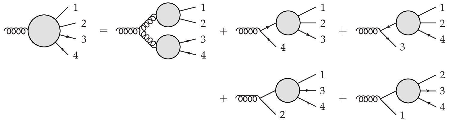
AVHLIB allows for various choices of the representation of the external helicities and colors. These include both the color-ordered representation [36, 37], with exact summation over color, and the color-dressed representation [38, 39], with Monte Carlo summation for large multiplicities. Helicity configurations can be summed exactly, or, again for large multiplicities, treated in a Monte Carlo approach, both discrete and with continuous random polarizations [40]. The library includes a full Monte Carlo program with an adaptive phase space generator [41, 42] that deals with the integration variables related to both the initial-state momenta and the final-state momenta.
The program can also conveniently generate a file of unweighted events, which approach was used for the analysis presented in this paper. In the present calculation we use: as the factorization scale and = 1.5 GeV in both -factorization and in the reference collinear-factorization calculations. Uncertainties related to the choice of the parameters were discussed e.g. in Ref. [33] and will be not considered here. Here we wish to concentrate on the relative effect and modifications with respect to the results of the collinear-factorization calculations presented already in the literature [32, 33].
III First Results
In this section we wish to compare the new results of the -factorization approach to those obtained by us in Ref. [33] in the collinear-factorization approach.
In Fig. 6 we show standard single particle distributions in charm quark/antiquark transverse momentum (left panel) and its rapidity (right panel). We predict an enhancement of the cross section at large transverse momenta of or compared to the collinear-factorization approach. The rapidity distributions in both approaches are rather similar (see the left panel of the figure).


Distributions in rapidity of the (or ) and , defined as and respectively, are shown in Fig. 7. The distributions are much narrower than those for single quark/antiquark which reflects the fact that the two different quarks (or two different antiquarks) have typically different rapidities. The discussed distributions in and would be identical only if (strong rapidity correlations). This will become clearer when inspecting rapidity difference in the next plots.


Similar distributions but for rapidity distance between two quarks (or two antiquarks) and between and are shown in Fig. 8. On average the distance between and is larger than that for and . This can be understood easily in the high-energy approximation discussed in Ref. [32] by inspecting the contributing diagrams. Some enhancement at small rapidity separations can be observed in the -factorization approach compared to the collinear approach.


The distributions in rapidity distance are strongly correlated with or distributions shown in Fig. 9. Those distribution are, however, difficult to measure as rather mesons are measured and not quarks or antiquarks.


Quite interesting are azimuthal angle correlations between and or and . The corresponding distributions are shown in Fig. 10. We note much bigger decorrelation of two quarks or and in the -factorization approach compared to the collinear approach. This is due to explict account of gluon virtualities (transverse momenta). We will return to this point when discussing azimuthal correlations between mesons at the end of this section.


Next we wish to visualize the regions of the transverse momenta of initial gluons that give sizeable contribution to the SPS cross section. In Fig. 11 we show a two-dimensional distribution in intial-gluon transverse momenta. The dependence on and shown in the figure is determineated by the UGDF used in the calculation as well as by the dependence of the matrix element on and . Other models of unintegrated gluon distributions would give different dependencies. Clearly we get large contributions from the regions far from the collinear case ( = 0 and = 0). This has of course consequences for other observables discussed above through the dependence of the matrix element on the gluon transverse momenta and its correlation with other kinematical variables.

We will not discuss in the present letter the correlations between the gluon virtualities (or their transverse momenta) and other kinematical variables related to the charm quarks and antiquarks.


So far we have considered production of quarks/antiquarks. As discussed in our previous paper [33] such a final states may lead to the production of two mesons, both containing quarks or both containing antiquarks which is not possible e.g. for the final-state case. As explained in Ref. [33] the DPS gives cross sections very similar to those measured by the LHCb collaboration [31]. How important is the SPS contribution discussed in this paper, calculated here in the -factorization, is shown in Fig. 12. For comparison we show also SPS results calculated in collinear-factorization approach [33]. The two approaches give somewhat different shapes of correlation observables, inspite that the integrated cross sections are rather similar as discussed already at the parton level. Our results, so far the most advanced in the literature as for as the SPS contribution is considered, are not able to explain discrepancy between DPS contribution and the LHCb experimental data. If the discrepancies are due to simplifications in the treatment of DPS requires further studies including for example spin and flavour correlations. Some works in this direction already started [43].
IV Conclusions
In the present paper we have made a first calculation of the cross section for in the -factorization approach, i.e. focussing on single parton scattering process. This is a first process for which -factorization is applied. In this calculation we have used the Kimber-Martin-Ryskin unintegrated gluon distribution(s) which effectively takes into account the dominant higher-order corrections. The off-shell matrix element was calculated using a new technique developed recently in Kraków.
The results of the -factorization approach were compared with the results of the collinear-factorization approach. In general, the -factorization results are only slightly bigger than those for collinear approach. An exception is the transverse momentum distribution above 10 GeV where a sizeable enhancement has been observed. Inclusion of gluon virtualities leads to a decorrelation in azimuthal angle between and or and .
Since the cross section is in general very similar as for the collinear-factorization approach we conclude that the final state at the LHC energies is dominantly produced by the double parton scattering as discussed in our recent papers, and the SPS contribution, although interesting by itself, is rather small. A comparison to predictions of double-parton scattering results and recent LHCb data for azimuthal angle correlations between and or and mesons strongly suggests that the assumption of two fully independent DPS () may be too approximate or even not valid. Some possible reasons were discussed in Ref. [43]. The effect found there is, however, too small to explain a rather large effect observed by the LHCb collaboration. This remains a challenge for future theoretical studies and should be confirmed by the LHCb collaboration at , TeV.
Acknowledgments
This study was partially supported by the Centre for Innovation and Transfer of Natural Sciences and Engineering Knowledge in Rzeszów. Graphs were drawn with the help of Jaxodraw.
References
- [1] S. Catani, M. Ciafaloni and F. Hautmann, Nucl. Phys. 366, 135 (1991).
- [2] J.C. Collins and R.K. Ellis, Nucl. Phys. B360, 3 (1991).
- [3] R.D. Ball and R.K. Ellis, J. High Energy Phys. 05, 053 (2001).
- [4]
Ph. Hägler, R. Kirschner, A. Schäfer, I. Szymanowski and O.V Teryaev,
Phys. Rev. D62, 071502 (2000). - [5] S.P. Baranov and M. Smizanska, Phys. Rev. D62, 014012 (2000).
- [6]
N. P. Zotov, A. V. Lipatov and V. A. Saleev,
Phys. Atom. Nucl. 66, 755 (2003)
[Yad. Fiz. 66, 786 (2003)]. - [7]
S.P. Baranov, A.V. Lipatov and N.P. Zotov, Phys. Atom. Nucl. 67, 837 (2004)
[Yad. Fiz. 67, 856 (2004)]. - [8] M. Łuszczak and A. Szczurek, Phys. Rev. D73, 054028 (2006).
- [9] Yu.M. Shabelski and A.G. Shuvaev, Phys. Atom. Nucl. 69, 314 (2006).
- [10] M. Łuszczak, R. Maciuła and A. Szczurek, Phys. Rev. D79, 034009 (2009).
- [11] R. Maciuła, A. Szczurek and G. Ślipek, Phys. Rev. D83, 054014 (2011).
- [12] R. S. Pasechnik, O. V. Teryaev and A. Szczurek, Eur. Phys. J. C 47, 429 (2006).
- [13] A. V. Lipatov, M. A. Malyshev and N. P. Zotov, Phys. Lett. B 735, 79 (2014).
- [14] A. Szczurek, M. Łuszczak and R. Maciuła, Phys. Rev. D 90, 094023 (2014).
- [15] M.A. Kimber, A.D. Martin and M.G. Ryskin, Phys. Rev. D63, 114027 (2001).
- [16]
H. Jung, M. Kraemer, A.V. Lipatov and N.P. Zotov, Phys. Rev. D85, 034035 (2012);
J. High Energy Phys. 01, 085 (2011). - [17] V. Saleev and A. Shipilova, Phys. Rev. D 86, 034032 (2012).
- [18] R. Maciuła, and A. Szczurek, Phys. Rev. D87, 094022 (2013).
- [19] A. V. Karpishkov, M. A. Nefedov, V. A. Saleev and A. V. Shipilova, Phys. Rev. D 91, 054009 (2015).
- [20] A. V. Karpishkov, M. A. Nefedov, V. A. Saleev and A. V. Shipilova, Int. J. Mod. Phys. A 30, 1550023 (2015).
- [21] S. P. Baranov, A. V. Lipatov and N. P. Zotov, Eur. Phys. J. C 56, 371 (2008).
- [22] A. van Hameren, P. Kotko and K. Kutak, Phys. Rev. D 88, 094001 (2013) [Phys. Rev. D 90, 039901 (2014)].
- [23] A. V. Lipatov and N. P. Zotov, arXiv:1501.05130 [hep-ph].
- [24] A. van Hameren, P. Kotko and K. Kutak, J. High Energy Phys. 01, 078 (2013) [arXiv:1211.0961 [hep-ph]].
- [25] A. van Hameren, J. High Energy Phys. 07, 138 (2014) [arXiv:1404.7818 [hep-ph]].
- [26] P. Kotko, J. High Energy Phys. 07, 128 (2014) [arXiv:1403.4824 [hep-ph]].
- [27] A. van Hameren, P. Kotko, K. Kutak, C. Marquet and S. Sapeta, Phys. Rev. D 89, 094014 (2014).
- [28] A. van Hameren, P. Kotko, K. Kutak and S. Sapeta, Phys. Lett. B 737, 335 (2014).
- [29] M. Łuszczak, R. Maciuła, and A. Szczurek, Phys. Rev. D85, 094034 (2012).
- [30] R. Maciuła, and A. Szczurek, Phys. Rev. D87, 074039 (2013).
- [31] R. Aaij et al. (LHCb Collaboration), J. High Energy Phys. 06, 141 (2012).
- [32] W. Schäfer, and A. Szczurek, Phys. Rev. D85, 094029 (2012).
- [33] A. van Hameren, R. Maciuła and A. Szczurek, Phys. Rev. D 89, 094019 (2014).
- [34] M. Bury and A. van Hameren, arXiv:1503.08612 [hep-ph].
- [35] F. Caravaglios and M. Moretti, Phys. Lett. B 358 (1995) 332 [hep-ph/9507237].
- [36] A. Kanaki and C. G. Papadopoulos, AIP Conf. Proc. 583 (2001) 169 [hep-ph/0012004].
- [37] F. Maltoni, K. Paul, T. Stelzer and S. Willenbrock, Phys. Rev. D 67 (2003) 014026 [hep-ph/0209271].
- [38] C. G. Papadopoulos and M. Worek, Eur. Phys. J. C 50 (2007) 843 [hep-ph/0512150].
- [39] C. Duhr, S. Hoeche and F. Maltoni, JHEP 0608 (2006) 062 [hep-ph/0607057].
- [40] P. Draggiotis, R. H. P. Kleiss and C. G. Papadopoulos, Phys. Lett. B 439 (1998) 157 [hep-ph/9807207].
- [41] A. van Hameren, Acta Phys. Polon. B 40 (2009) 259 [arXiv:0710.2448 [hep-ph]].
- [42] A. van Hameren, arXiv:1003.4953 [hep-ph].
- [43] M G. Echevarria, T. Kasemets, P. J. Mulders and C. Pisano, J. High Energy Phys. 04, 034 (2015).