跳到论文正文
W Papers独立论文阅读器 arXiv:1504.06459 论文正文 计算阅读时间 · 0%
引用这篇论文根据当前论文元数据生成,正式投稿前建议核对。


License: arXiv.org perpetual non-exclusive license
arXiv:1504.06459v2 [quant-ph] 19 Jul 2016

kk-extendibility of high-dimensional bipartite quantum states

Cécilia Lancien Address: Cécilia Lancien: Institut Camille Jordan, Université Claude Bernard Lyon 1, 69622 Villeurbanne Cedex, France & Física Teòrica: Informació i Fenòmens Quàntics, Universitat Autònoma de Barcelona, 08193 Bellaterra (Barcelona), Spain. Email address: lancien@math.univ-lyon1.fr
Abstract.

The idea of detecting the entanglement of a given bipartite state by searching for symmetric extensions of this state was first proposed by Doherty, Parrilo and Spedialeri. The complete family of separability tests it generates, often referred to as the hierarchy of kk-extendibility tests, has already proved to be most promising. The goal of this paper is to try and quantify the efficiency of this separability criterion in typical scenarios. For that, we essentially take two approaches. First, we compute the average width of the set of kk-extendible states, in order to see how it scales with the one of separable states. And second, we characterize when random-induced states are, depending on the ancilla dimension, with high probability violating or not the kk-extendibility test, and compare the obtained result with the corresponding one for entanglement vs separability. The main results can be precisely phrased as follows: on 𝐂d⊗𝐂d\mathbf{C}^{d}\otimes\mathbf{C}^{d}, when dd grows, the average width of the set of kk-extendible states is equivalent to (2/k)/d(2/\sqrt{k})/d, while random states obtained as partial traces over an environment 𝐂s\mathbf{C}^{s} of uniformly distributed pure states are violating the kk-extendibility test with probability going to 11 if s<((k−1)2/4​k)​d2s<((k-1)^{2}/4k)d^{2}. Both statements converge to the conclusion that, if kk is fixed, kk-extendibility is asymptotically a weak approximation of separability, even though any of the other well-studied separability relaxations is outperformed by kk-extendibility as soon as kk is above a certain (dimension independent) value.

1. Introduction

Deciding whether a given bipartite quantum state is entangled or separable (or even just close to separable) is known to be a computationally hard task (see [19] and [17]). Several much more easily checkable necessary conditions for separability do exist though, the most famous and widely used ones being perhaps the positivity of partial transpose criterion [31], the realignment criterion [11] or the kk-extendibility criterion [15]. All of them have in common that verifying if a given state fulfils them or not may be cast as a Semi-Definite Program (SDP) and hence be efficiently solved (see e.g. the quite extensive review [14] for much more on that topic).

We focus here on a relaxation of the notion of separability of quite different kind: the so-called kk-extendibility criterion for separability, which was introduced in [15]. It is especially appealing because it provides a hierarchy of increasingly powerful separability tests (expressible as SDPs of increasing dimension), which is additionally complete, meaning that any entangled state is guaranteed to fail a test after some finite number of steps in the hierarchy. Let us be more precise.

Definition 1.1.

Let k∈𝐍k\in\mathbf{N}. A state ρAB\rho_{\mathrm{A}\mathrm{B}} on a bipartite Hilbert space A⊗B\mathrm{A}\otimes\mathrm{B} is kk-extendible with respect to B\mathrm{B} if there exists a state ρABk\rho_{\mathrm{A}\mathrm{B}^{k}} on A⊗B⊗k\mathrm{A}\otimes\mathrm{B}^{\otimes k} which is invariant under any permutation of the B\mathrm{B} subsystems and such that ρAB=TrBk−1⁡ρABk\rho_{\mathrm{A}\mathrm{B}}=\tr_{\mathrm{B}^{k-1}}\rho_{\mathrm{A}\mathrm{B}^{k}}.

Theorem 1.2 (The complete family of kk-extendibility criteria for separability, [15]).

A state on a bipartite Hilbert space A⊗B\mathrm{A}\otimes\mathrm{B} is separable if and only if it is kk-extendible with respect to B\mathrm{B} for all k∈𝐍k\in\mathbf{N}.

Note that one direction in Theorem 1.2 is obvious, namely that a separable state on some bipartite system is necessarily kk-extendible for all k∈𝐍k\in\mathbf{N} (with respect to both subsystems). Indeed, if ρ=∑xpx​σx⊗τx\rho=\sum_{x}p_{x}\sigma_{x}\otimes\tau_{x} is separable, then ∑xpx​σx⊗k⊗τx\sum_{x}p_{x}\sigma_{x}^{\otimes k}\otimes\tau_{x} and ∑xpx​σx⊗τx⊗k\sum_{x}p_{x}\sigma_{x}\otimes\tau_{x}^{\otimes k} are symmetric extensions of ρ\rho to kk copies of the first and second subsystems respectively. The other direction in Theorem 1.2 follows from the quantum finite de Finetti theorem (see e.g. [24, 12] for the seminal statements). The latter establishes, roughly speaking, that starting from a permutation-invariant state on some tensor power system and tracing out all except a few of the subsystems, one gets a state that may be well-approximated by a convex combination of tensor power states (with a vanishing error as the initial number of subsystems increases).

It is easy to see that if a state is kk-extendible for some k∈𝐍k\in\mathbf{N}, then it is automatically k′k^{\prime}-extendible for all k′⩽kk^{\prime}\leqslant k. Hence, the necessary and sufficient condition for separability provided by Theorem 1.2 actually decomposes into a series of increasingly constraining necessary conditions for separability, which are only asymptotically also sufficient (see Figure 1). In real life however, checks can only be done up to a finite level in this hierarchy. It thus makes sense to ask, given a finite k∈𝐍k\in\mathbf{N}, how “powerful” the kk-extendibility test is to detect entanglement.

Figure 1. The nested and converging sequence of kk-extendibility relaxations of separability, k∈𝐍k\in\mathbf{N}
Refer to caption

Actually, various more quantitative versions of Theorem 1.2 do exist, that put bounds on how far a kk-extendible state can be from separable. Let us mention two quite different statements in that direction. The original result, appearing in [12], establishes that a state on A⊗B\mathrm{A}\otimes\mathrm{B} which is kk-extendible with respect to B\mathrm{B} is at distance at most 2​dB2/k2d_{\mathrm{B}}^{2}/k, in 11-norm, from the set of separable states. It is a direct consequence of one of the quantitative versions of the quantum finite De Finetti theorem. A more recent result, proved essentially in [9] and improved in [10], stipulates that such a state is at distance at most 2​ln⁡dA/k\sqrt{2\ln d_{\mathrm{A}}/k}, in 𝐋𝐎𝐂𝐂→\mathbf{LOCC}^{\rightarrow}-norm, from the set of separable states (see e.g. [3] for a precise definition of the operational one-way-LOCC norm). It relies on the observation that a kk-extendible state has a small squashed entanglement, and therefore cannot be distinguished well from a separable state by local observers. The main problem of such estimates is that they become non-trivial only when k≫dBk\gg d_{\mathrm{B}} or k≫ln⁡dAk\gg\ln d_{\mathrm{A}}. So in the case where dA,dBd_{\mathrm{A}},d_{\mathrm{B}} are “big”, can anything interesting still be said for a “not too big” kk? On the other hand, these bounds valid for any kk-extendible state are known to be close from optimal (there are examples of kk-extendible states whose closest separable state is at distance of order dB/kd_{\mathrm{B}}/k in 11-norm or of order ln⁡dA/k\sqrt{\ln d_{\mathrm{A}}/k} in 𝐋𝐎𝐂𝐂→\mathbf{LOCC}^{\rightarrow}-norm). Consequently, one may only hope to make stronger statements about average behaviours.

This is precisely the general question we address here, being especially interested in the case of high-dimensional bipartite quantum systems. We try and quantify in two distinct ways the typical efficiency of the kk-extendibility criterion for separability in this asymptotic regime.

The first approach consists in estimating a specific size parameter (known as the mean width) of the set of kk-extendible states when the dimension of the underlying Hilbert space goes to infinity. Comparing the obtained value with the known asymptotic estimate for the mean width of the set of separable states then tells us how the sizes of these two sets of states scale with one another. The computation is carried out in Section 2 (where all needed notions related to high-dimensional convex geometry are properly defined as well) and ends with the concluding Theorem 2.5, some technical parts being relegated to Appendix D. In Section 3, the result is commented and comparisons are made between the mean-widths of, on the one hand, kk-extendible states, and on the other, separable or PPT states. Besides, a smaller upper bound is derived, in Section 4 and its companion technical Appendix E, on the mean width of the set of kk-extendible states whose extension is required to be PPT (precise definitions and motivations to look at this set of states appear there).

The second approach consists in looking at random mixed states which are obtained by partial tracing over an ancilla space a uniformly distributed pure state, and characterizing when these are, with overwhelming probability as the dimension of the system grows, kk-extendible or not. Again, comparing the obtained result with the known one for separability provides some information on how powerful the kk-extendibility test is to detect entanglement. Section 5 introduces all required material regarding the considered model of random-induced states and one possible way of detecting their non-kk-extendibility. The adopted strategy is next seen through in Section 6, relying on technical statements put in Appendix F, and concludes as Theorem 6.4. The determined environment dimension below which random-induced states are with high probability violating the kk-extendibility criterion is then compared, in Section 7, with the previously established ones for violating other separability criteria, and for actually not being separable.

Finally, generalizations to the unbalanced case are stated in Section 8 (Theorems 8.1 and 8.2), while Section 9 exposes miscellaneous concluding remarks and loose ends.

The reader may have a look at Table 1 for a sample corollary of this study.

Table 1. Comparison of the average and typical case performance of the kk-extendibility criterion with that of the PPT and realignment criteria
k mean width of the set entanglement detection of random states
PPT for k⩾11k\geqslant 11 for k⩾17k\geqslant 17
realignment ? for k⩾5k\geqslant 5

Appendix A gathers a bunch of standard definitions and facts about the combinatorics of permutations and partitions which are necessary for our purposes. All employed notation on that matter are also introduced there. In Appendix B, the connection is made between computing moments of GUE or Wishart matrices and counting permutations having a certain genus. These general observations play a key role in the moments’ derivations of Appendices D, E and F, which are, as for them, specifically the ones that we need to obtain our various statements. To get tractable expressions, though, a formula relating the number of cycles in some specific permutations is additionally required, whose proof is detailed in Appendix C. Appendix G, finally, is devoted to establishing the last crucial ingredient in most of our reasonings, namely bounding the number of non-geodesic permutations (in terms of the number of geodesic ones) in some particular instances which are of interest to us. Aside, Appendix H is dedicated to proving more precise results than the ones which are strictly needed on the convergence of the studied random matrix ensembles, and in generalizing the developed method to establish the asymptotic freeness of certain gaussian random matrices.

Notation

For any Hilbert space H≡𝐂n\mathrm{H}\equiv\mathbf{C}^{n}, we shall denote by ℋ⁡(H)≡ℋ⁡(n)\mathcal{H}(\mathrm{H})\equiv\mathcal{H}(n) the set of Hermitian operators on H\mathrm{H}, and by ℋ+​(H)≡ℋ+​(n)\mathcal{H}_{+}(\mathrm{H})\equiv\mathcal{H}_{+}(n) the subset of positive operators on H\mathrm{H}. For each p∈𝐍p\in\mathbf{N}, we define ∥⋅∥p\|\cdot\|_{p} as the Schatten pp-norm on ℋ⁡(H)\mathcal{H}(\mathrm{H}), i.e. ∥⋅∥p=(Tr[|⋅|p])1/p\|\cdot\|_{p}=\left(\tr\left[|\cdot|^{p}\right]\right)^{1/p}, and ∥⋅∥∞=limp→+∞∥⋅∥p\|\cdot\|_{\infty}=\lim_{p\rightarrow+\infty}\|\cdot\|_{p}. Particular instances of interest are the trace class norm ∥⋅∥1\|\cdot\|_{1}, the Hilbert–Schmidt norm ∥⋅∥2\|\cdot\|_{2}, and the operator norm ∥⋅∥∞\|\cdot\|_{\infty}. We shall also denote by 𝒟⁡(H)≡𝒟⁡(n)\mathcal{D}(\mathrm{H})\equiv\mathcal{D}(n) the set of states on H\mathrm{H} (positive and trace 11 operators).

We will in fact mostly consider the case where H=A⊗B≡𝐂d⊗𝐂d\mathrm{H}=\mathrm{A}\otimes\mathrm{B}\equiv\mathbf{C}^{d}\otimes\mathbf{C}^{d} is a (balanced) bipartite Hilbert space. And we introduce the additional notations 𝒮⁡(A:B)≡𝒮⁡(d×d)\mathcal{S}(\mathrm{A}:\mathrm{B})\equiv\mathcal{S}(d\times d) for the set of separable states on H\mathrm{H}, 𝒫⁡(A:B)≡𝒫⁡(d×d)\mathcal{P}(\mathrm{A}:\mathrm{B})\equiv\mathcal{P}(d\times d) for the set of PPT states on H\mathrm{H} (in both cases in the cut A:B\mathrm{A}:\mathrm{B}), and for each k∈𝐍k\in\mathbf{N}, ℰk​(A:B)≡ℰk​(d×d)\mathcal{E}_{k}(\mathrm{A}:\mathrm{B})\equiv\mathcal{E}_{k}(d\times d) for the set of kk-extendible states on H\mathrm{H} (in the cut A:B\mathrm{A}:\mathrm{B} and with respect to B\mathrm{B}).

Preliminary technical lemma

It will be essential for us in the sequel to express in a more tractable way the quantity supσ∈ℰk​(A:B)Tr(Mσ)\sup_{\sigma\in\mathcal{E}_{k}(\mathrm{A}{:}\mathrm{B})}\mathrm{Tr}(M\sigma), for any given Hermitian MM on A⊗B\mathrm{A}\otimes\mathrm{B}. Such amenable expression is provided by Lemma 1.3 below.

Lemma 1.3.

Let k∈𝐍k\in\mathbf{N}. For any MAB∈ℋ⁡(A⊗B)M_{\mathrm{A}\mathrm{B}}\in\mathcal{H}(\mathrm{A}\otimes\mathrm{B}), we have

supσAB∈ℰk​(A:B)Tr(MABσAB)=‖1k∑j=1𝑘M~ABk(j)‖∞,\underset{\sigma_{\mathrm{A}\mathrm{B}}\in\mathcal{E}_{k}(\mathrm{A}{:}\mathrm{B})}{\sup}\ \tr\big(M_{\mathrm{A}\mathrm{B}}\sigma_{\mathrm{A}\mathrm{B}}\big)=\left\|\frac{1}{k}\underset{j=1}{\overset{k}{\sum}}\widetilde{M}_{\mathrm{A}\mathrm{B}^{k}}(j)\right\|_{\infty},

where for each 1⩽j⩽k1\leqslant j\leqslant k, denoting by IdB^jk\mathrm{Id}_{\widehat{\mathrm{B}}^{k}_{j}} the identity on B1⊗⋯⊗Bj−1⊗Bj+1⊗⋯⊗Bk\mathrm{B}_{1}\otimes\cdots\otimes\mathrm{B}_{j-1}\otimes\mathrm{B}_{j+1}\otimes\cdots\otimes\mathrm{B}_{k}, we defined M~ABk​(j)=MABj⊗IdB^jk\widetilde{M}_{\mathrm{A}\mathrm{B}^{k}}(j)=M_{\mathrm{A}\mathrm{B}_{j}}\otimes\mathrm{Id}_{\widehat{\mathrm{B}}^{k}_{j}}.

Before proving Lemma 1.3, let us introduce once and for all the following notation, which we shall later use on several occasions: for any MABk∈ℋ⁡(A⊗B⊗k)M_{\mathrm{A}\mathrm{B}^{k}}\in\mathcal{H}(\mathrm{A}\otimes\mathrm{B}^{\otimes k}), we define its symmetrisation with respect to B⊗k\mathrm{B}^{\otimes k} as

SymA:Bk(MABk)=1k!∑π∈𝔖⁡(k)(IdA⊗U(π)Bk)MABk(IdA⊗U(π)Bk)†,\Sym_{\mathrm{A}{:}\mathrm{B}^{k}}(M_{\mathrm{A}\mathrm{B}^{k}})=\frac{1}{k!}\underset{\pi\in\mathfrak{S}(k)}{\sum}\big(\mathrm{Id}_{\mathrm{A}}\otimes U(\pi)_{\mathrm{B}^{k}}\big)M_{\mathrm{A}\mathrm{B}^{k}}\big(\mathrm{Id}_{\mathrm{A}}\otimes U(\pi)_{\mathrm{B}^{k}}\big)^{\dagger},

where for each permutation π∈𝔖⁡(k)\pi\in\mathfrak{S}(k), U​(π)BkU(\pi)_{\mathrm{B}^{k}} denotes the associated permutation unitary on B⊗k\mathrm{B}^{\otimes k} (see e.g. [21] for further details).

Proof.

By definition, the condition σAB∈ℰk​(A:B)\sigma_{\mathrm{A}\mathrm{B}}\in\mathcal{E}_{k}(\mathrm{A}{:}\mathrm{B}) is equivalent to the condition σAB=TrBk−1SymA:Bk(σABk)\sigma_{\mathrm{A}\mathrm{B}}=\tr_{\mathrm{B}^{k-1}}\Sym_{\mathrm{A}{:}\mathrm{B}^{k}}(\sigma_{\mathrm{A}\mathrm{B}^{k}}) for some σABk∈𝒟⁡(A⊗B⊗k)\sigma_{\mathrm{A}\mathrm{B}^{k}}\in\mathcal{D}(\mathrm{A}\otimes\mathrm{B}^{\otimes k}). Hence, for any MAB∈ℋ⁡(A⊗B)M_{\mathrm{A}\mathrm{B}}\in\mathcal{H}(\mathrm{A}\otimes\mathrm{B}), we have

supσAB∈ℰk​(A:B)TrAB[MABσAB]\displaystyle\underset{\sigma_{\mathrm{A}\mathrm{B}}\in\mathcal{E}_{k}(\mathrm{A}{:}\mathrm{B})}{\sup}\ \tr_{\mathrm{A}\mathrm{B}}\big[M_{\mathrm{A}\mathrm{B}}\sigma_{\mathrm{A}\mathrm{B}}\big] =supσABk∈𝒟⁡(A⊗B⊗k)TrAB[MABTrBk−1SymA:Bk(σABk)]\displaystyle=\underset{\sigma_{\mathrm{A}\mathrm{B}^{k}}\in\mathcal{D}(\mathrm{A}\otimes\mathrm{B}^{\otimes k})}{\sup}\ \tr_{\mathrm{A}\mathrm{B}}\big[M_{\mathrm{A}\mathrm{B}}\tr_{\mathrm{B}^{k-1}}\Sym_{\mathrm{A}{:}\mathrm{B}^{k}}(\sigma_{\mathrm{A}\mathrm{B}^{k}})\big]
=supσABk∈𝒟⁡(A⊗B⊗k)TrABk[(MAB⊗IdBk−1)SymA:Bk(σABk)]\displaystyle=\underset{\sigma_{\mathrm{A}\mathrm{B}^{k}}\in\mathcal{D}(\mathrm{A}\otimes\mathrm{B}^{\otimes k})}{\sup}\ \tr_{\mathrm{A}\mathrm{B}^{k}}\big[\big(M_{\mathrm{A}\mathrm{B}}\otimes\mathrm{Id}_{\mathrm{B}^{k-1}}\big)\Sym_{\mathrm{A}{:}\mathrm{B}^{k}}(\sigma_{\mathrm{A}\mathrm{B}^{k}})\big]
=supσABk∈𝒟⁡(A⊗B⊗k)TrABk[SymA:Bk(MAB⊗IdBk−1)σABk]\displaystyle=\underset{\sigma_{\mathrm{A}\mathrm{B}^{k}}\in\mathcal{D}(\mathrm{A}\otimes\mathrm{B}^{\otimes k})}{\sup}\ \tr_{\mathrm{A}\mathrm{B}^{k}}\big[\Sym_{\mathrm{A}{:}\mathrm{B}^{k}}\big(M_{\mathrm{A}\mathrm{B}}\otimes\mathrm{Id}_{\mathrm{B}^{k-1}}\big)\sigma_{\mathrm{A}\mathrm{B}^{k}}\big]
=‖SymA:Bk(MAB⊗IdBk−1)‖∞.\displaystyle=\left\|\Sym_{\mathrm{A}{:}\mathrm{B}^{k}}\big(M_{\mathrm{A}\mathrm{B}}\otimes\mathrm{Id}_{\mathrm{B}^{k-1}}\big)\right\|_{\infty}.

Now, for each π∈𝔖⁡(k)\pi\in\mathfrak{S}(k), (IdA⊗U​(π)Bk)​(MAB⊗IdBk−1)​(IdA⊗U​(π)Bk)†=MABπ⁡(1)⊗IdB^π⁡(1)k\big(\mathrm{Id}_{\mathrm{A}}\otimes U(\pi)_{\mathrm{B}^{k}}\big)\big(M_{\mathrm{A}\mathrm{B}}\otimes\mathrm{Id}_{\mathrm{B}^{k-1}}\big)\big(\mathrm{Id}_{\mathrm{A}}\otimes U(\pi)_{\mathrm{B}^{k}}\big)^{\dagger}=M_{\mathrm{A}\mathrm{B}_{\pi(1)}}\otimes\mathrm{Id}_{\widehat{\mathrm{B}}^{k}_{\pi(1)}}. Therefore, grouping together, for each 1⩽j⩽k1\leqslant j\leqslant k, the permutations π∈𝔖⁡(k)\pi\in\mathfrak{S}(k) such that π⁡(1)=j\pi(1)=j, we get

SymA:Bk(MAB⊗IdBk−1)=1k∑j=1kMABj⊗IdB^jk,\Sym_{\mathrm{A}{:}\mathrm{B}^{k}}\big(M_{\mathrm{A}\mathrm{B}}\otimes\mathrm{Id}_{\mathrm{B}^{k-1}}\big)=\frac{1}{k}\sum_{j=1}^{k}M_{\mathrm{A}\mathrm{B}_{j}}\otimes\mathrm{Id}_{\widehat{\mathrm{B}}^{k}_{j}},

and hence the advertised result. ∎

2. Mean width of the set of kk-extendible states for “small” kk

2.1. Preliminaries on convex geometry

Let us introduce a few notions coming from classical convex geometry which we shall need in the sequel. For any K⊂ℋ⁡(𝐂n)K\subset\mathcal{H}(\mathbf{C}^{n}) and any M∈ℋ⁡(𝐂n)M\in\mathcal{H}(\mathbf{C}^{n}) having unit Hilbert–Schmidt norm, we define the width of KK in the direction MM as

w⁡(K,M)=supΔ∈K​Tr​(M​Δ).w(K,M)=\underset{\Delta\in K}{\sup}\mathrm{Tr}(M\Delta).

The mean width of KK is then defined as the average of w⁡(K,⋅)w(K,\cdot) over the whole Hilbert–Schmidt unit sphere SH​S​(𝐂n)S_{HS}(\mathbf{C}^{n}) of ℋ⁡(𝐂n)\mathcal{H}(\mathbf{C}^{n}) (equipped with the Haar measure σ\sigma) i.e.

w⁡(K)=∫M∈SH​S​(𝐂n)w⁡(K,M)​𝑑σ​(M)=∫M∈SH​S​(𝐂n)[supΔ∈K​Tr​(M​Δ)]​𝑑σ​(M).w(K)=\int_{M\in S_{HS}(\mathbf{C}^{n})}w(K,M)\mathrm{d}\sigma(M)=\int_{M\in S_{HS}(\mathbf{C}^{n})}\left[\underset{\Delta\in K}{\sup}\mathrm{Tr}(M\Delta)\right]\mathrm{d}\sigma(M).

This average width ww is an interesting size parameter, on its own, but also because it is related to other important geometric quantities, such as e.g. the volume radius vrad\mathrm{vrad}, which is defined as the radius of the Euclidean ball having same volume (i.e. Lebesgue measure). For instance, we have for any convex body KK the Urysohn inequality w⁡(K)⩾vrad⁡(K)w(K)\geqslant\mathrm{vrad}(K), and for most of the convex bodies KK we shall be considering a “reverse” Urysohn inequality w⁡(K)⩽μ​vrad​(K)w(K)\leqslant\mu\,\mathrm{vrad}(K) for some μ⩾1\mu\geqslant 1. These connections and the precise formulation of these convex geometry results are exemplified in Section 3.

In order to compute the quantity w⁡(K)w(K), it is often convenient to re-express it as a Gaussian rather than spherical averaging. We thus denote by G​U​E​(n)GUE(n) the Gaussian Unitary Ensemble on 𝐂n\mathbf{C}^{n}, which is the standard Gaussian vector in ℋ⁡(𝐂n)\mathcal{H}(\mathbf{C}^{n}) (equivalently, G∼G​U​E​(n)G\sim GUE(n) if G=(H+H†)/2G=(H+H^{\dagger})/\sqrt{2} with HH a n×nn\times n matrix having independent complex normal entries). And we define the Gaussian mean width of KK as

wG​(K)=𝐄G∼GUE⁡(n)⁡[supΔ∈K​Tr​(G​Δ)].w_{G}(K)=\E_{G\sim GUE(n)}\left[\underset{\Delta\in K}{\sup}\mathrm{Tr}(G\Delta)\right].

Just observing that for G∼G​U​E​(n)G\sim GUE(n), G/‖G‖2G/\|G\|_{2} is uniformly distributed over SH​S​(𝐂n)S_{HS}(\mathbf{C}^{n}), and G/‖G‖2G/\|G\|_{2}, ‖G‖2\|G\|_{2} are independent random variables, we get that the link between both quantities is, setting γ⁡(n)=𝐄G∼GUE⁡(n)⁡‖G‖2\gamma(n)=\E_{G\sim GUE(n)}\|G\|_{2}, which is known to satisfy γ(n)∼n→+∞n\gamma(n)\sim_{n\rightarrow+\infty}n (see e.g. [1], Chapter 2, for a proof),

(1) w⁡(K)=1γ⁡(n)​wG​(K).w(K)=\frac{1}{\gamma(n)}w_{G}(K).
Remark 2.1.

All the sets KK that we will consider in the sequel will actually be subsets of 𝒟⁡(𝐂n)\mathcal{D}(\mathbf{C}^{n}), hence living in the hyperplane of ℋ⁡(𝐂n)\mathcal{H}(\mathbf{C}^{n}) composed of trace 11 elements, i.e. in a space of real dimension n2−1n^{2}-1, rather than n2n^{2}. It would thus seem more natural to define their mean width w⁡(K)w(K) as an average width over a n2−2n^{2}-2, rather than n2−1n^{2}-1, dimensional Euclidean unit sphere. The Gaussian mean width wG​(K)w_{G}(K), on the other hand, is an intrinsic notion that does not depend on the ambient dimension (because marginals of standard Gaussian vectors are themselves standard Gaussian vectors). As a consequence, we see from equation (1) that computing the mean width of KK as if it was a n2n^{2} dimensional set is asymptotically equivalent to computing it taking into account that it is in fact a n2−1n^{2}-1 dimensional set. We may therefore serenely forget about this issue.

Our aim is now to estimate, for any fixed k∈𝐍k\in\mathbf{N}, the mean width of the set of kk-extendible states on A⊗B\mathrm{A}\otimes\mathrm{B} when A≡B≡𝐂d\mathrm{A}\equiv\mathrm{B}\equiv\mathbf{C}^{d} and d→+∞d\rightarrow+\infty. By the definitions above, we have

w(ℰk(A:B))=1γ⁡(d2)𝐄GAB∼G​U​E​(d2)[supσAB∈ℰk​(A:B)Tr(GABσAB)].w\big(\mathcal{E}_{k}(\mathrm{A}{:}\mathrm{B})\big)=\frac{1}{\gamma(d^{2})}\mathbf{E}_{G_{\mathrm{A}\mathrm{B}}\sim GUE(d^{2})}\left[\underset{\sigma_{\mathrm{A}\mathrm{B}}\in\mathcal{E}_{k}(\mathrm{A}{:}\mathrm{B})}{\sup}\mathrm{Tr}\big(G_{\mathrm{A}\mathrm{B}}\sigma_{\mathrm{A}\mathrm{B}}\big)\right].

Using the result of Lemma 1.3, and the notation introduced there, we thus get,

(2) w⁡(ℰk​(A:B))=1γ⁡(d2)​𝐄GAB∼G​U​E​(d2)​‖1k​∑j=1𝑘​G~ABk​(j)‖∞.w\big(\mathcal{E}_{k}(\mathrm{A}{:}\mathrm{B})\big)=\frac{1}{\gamma(d^{2})}\mathbf{E}_{G_{\mathrm{A}\mathrm{B}}\sim GUE(d^{2})}\left\|\frac{1}{k}\underset{j=1}{\overset{k}{\sum}}\widetilde{G}_{\mathrm{A}\mathrm{B}^{k}}(j)\right\|_{\infty}.

2.2. An operator-norm estimate

As justified above, to obtain the mean width of the set of kk-extendible states on 𝐂d⊗𝐂d\mathbf{C}^{d}\otimes\mathbf{C}^{d}, what we need is to compute the average operator-norm 𝐄​‖∑j=1kG~ABk​(j)‖∞\mathbf{E}\left\|\sum_{j=1}^{k}\widetilde{G}_{\mathrm{A}\mathrm{B}^{k}}(j)\right\|_{\infty}, for GG a GUE matrix on 𝐂d⊗𝐂d\mathbf{C}^{d}\otimes\mathbf{C}^{d}. We will show that the following asymptotic estimate holds.

Proposition 2.2.

Fix k∈𝐍k\in\mathbf{N}. Then,

𝐄GAB∼G​U​E​(d2)​‖∑j=1𝑘​G~ABk​(j)‖∞​∼d→+∞​2​k​d.\mathbf{E}_{G_{\mathrm{A}\mathrm{B}}\sim GUE(d^{2})}\left\|\underset{j=1}{\overset{k}{\sum}}\widetilde{G}_{\mathrm{A}\mathrm{B}^{k}}(j)\right\|_{\infty}\underset{d\rightarrow+\infty}{\sim}2\sqrt{k}d.

As a preliminary step towards estimating the sup-norm 𝐄​‖∑j=1kG~ABk​(j)‖∞\mathbf{E}\left\|\sum_{j=1}^{k}\widetilde{G}_{\mathrm{A}\mathrm{B}^{k}}(j)\right\|_{\infty}, we will look at the 2​p2p-order moments 𝐄​Tr​[(∑j=1kG~ABk​(j))2​p]\mathbf{E}\,\mathrm{Tr}\left[\left(\sum_{j=1}^{k}\widetilde{G}_{\mathrm{A}\mathrm{B}^{k}}(j)\right)^{2p}\right], p∈𝐍p\in\mathbf{N}, and show that they can be expressed in terms of the 2​p2p-order moments of a centered semicircular distribution of appropriate parameter.

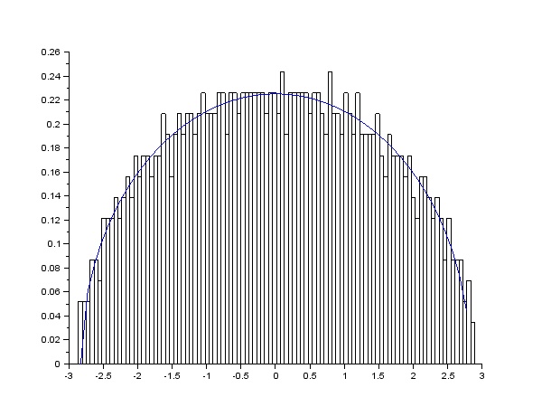
So let us recall first a few required definitions. For any σ>0\sigma>0, we shall denote by μS​C​(σ2)\mu_{SC(\sigma^{2})} the centered semicircular distribution of variance parameter σ2\sigma^{2}, whose density is given by

d​μS​C​(σ2)​(x)=12​π​σ2​4​σ2−x2​𝟏[−2​σ,2​σ]​(x)​d​x.\mathrm{d}\mu_{SC(\sigma^{2})}(x)=\frac{1}{2\pi\sigma^{2}}\sqrt{4\sigma^{2}-x^{2}}\mathbf{1}_{[-2\sigma,2\sigma]}(x)\mathrm{d}x.

We shall also denote, for each p∈𝐍p\in\mathbf{N}, by MS​C​(σ2)(p)\mathrm{M}_{SC(\sigma^{2})}^{(p)} its pp-order moment, i.e.  MS​C​(σ2)(p)=∫−∞+∞xp​d​μS​C​(σ2)​(x)\mathrm{M}_{SC(\sigma^{2})}^{(p)}=\int_{-\infty}^{+\infty}x^{p}\mathrm{d}\mu_{SC(\sigma^{2})}(x). It is well-known that

∀p∈𝐍,MS​C​(σ2)(2​p−1)=0andMS​C​(σ2)(2​p)=σ2​pCatp,\forall\ p\in\mathbf{N},\ \mathrm{M}_{SC(\sigma^{2})}^{(2p-1)}=0\ \ \text{and}\ \ \mathrm{M}_{SC(\sigma^{2})}^{(2p)}=\sigma^{2p}\,\mathrm{Cat}_{p},

where Catp\mathrm{Cat}_{p} is the pthp^{\text{th}} Catalan number defined in Lemma A.4.

Proposition 2.3.

Fix k∈𝐍k\in\mathbf{N}. Then, when d→+∞d\rightarrow+\infty, the random matrix (∑j=1kG~ABk​(j))/d\left(\sum_{j=1}^{k}\widetilde{G}_{\mathrm{A}\mathrm{B}^{k}}(j)\right)/d converges in moments towards a centered semicircular distribution of parameter kk. Equivalently, this means that, for any p∈𝐍p\in\mathbf{N},

𝐄GAB∼G​U​E​(d2)​Tr​[(∑j=1𝑘​G~ABk​(j))2​p−1]=0and𝐄GAB∼G​U​E​(d2)​Tr​[(∑j=1𝑘​G~ABk​(j))2​p]​∼d→+∞​MS​C​(k)(2​p)​d2​p+k+1.\mathbf{E}_{G_{\mathrm{A}\mathrm{B}}\sim GUE(d^{2})}\,\mathrm{Tr}\left[\left(\underset{j=1}{\overset{k}{\sum}}\widetilde{G}_{\mathrm{A}\mathrm{B}^{k}}(j)\right)^{2p-1}\right]=0\ \ \text{and}\ \ \mathbf{E}_{G_{\mathrm{A}\mathrm{B}}\sim GUE(d^{2})}\,\mathrm{Tr}\left[\left(\underset{j=1}{\overset{k}{\sum}}\widetilde{G}_{\mathrm{A}\mathrm{B}^{k}}(j)\right)^{2p}\right]\underset{d\rightarrow+\infty}{\sim}\mathrm{M}_{SC(k)}^{(2p)}d^{2p+k+1}.
Remark 2.4.

Stronger convergence results than the one established in Proposition 2.3 may in fact be proved, as discussed in Appendix H.

Proof of Proposition 2.3.

Let p∈𝐍p\in\mathbf{N}. Computing the value of the 2​p2p-order moment 𝐄​Tr​[(∑j=1kG~ABk​(j))2​p]\mathbf{E}\,\mathrm{Tr}\left[\left(\sum_{j=1}^{k}\widetilde{G}_{\mathrm{A}\mathrm{B}^{k}}(j)\right)^{2p}\right] may be done using the Gaussian Wick formula (see Lemma B.1 for the statement and Appendix B.1 for a succinct summary of how to derive moments of GUE matrices from it). In our case, what we get by the computations carried out in Appendix D and summarized in Proposition D.1 is that, for any d∈𝐍d\in\mathbf{N}, denoting by ♯⁡(⋅)\sharp(\cdot) the number of cycles in a permutation,

(3) 𝐄​Tr​[(∑j=1kG~ABk​(j))2​p]\displaystyle\mathbf{E}\,\mathrm{Tr}\left[\left(\sum_{j=1}^{k}\widetilde{G}_{\mathrm{A}\mathrm{B}^{k}}(j)\right)^{2p}\right] =∑f:[2​p]→[k]𝐄Tr[∏→i=12​pG~ABk(f(i))]\displaystyle=\sum_{f:[2p]\rightarrow[k]}\mathbf{E}\,\mathrm{Tr}\left[\underset{i=1}{\overset{2p}{\overrightarrow{\prod}}}\widetilde{G}_{\mathrm{A}\mathrm{B}^{k}}(f(i))\right]
(4) =∑f:[2​p]→[k]∑λ∈𝔓(2)​(2​p)d♯⁡(γ−1​λ)+♯⁡(γf−1​λ)+k−|Im⁡(f)|,\displaystyle=\underset{f:[2p]\rightarrow[k]}{\sum}\underset{\lambda\in\mathfrak{P}^{(2)}(2p)}{\sum}d^{\sharp(\gamma^{-1}\lambda)+\sharp(\gamma_{f}^{-1}\lambda)+k-|\im(f)|},

where we defined on {1,…,2​p}\{1,\ldots,2p\}, 𝔓(2)​(2​p)\mathfrak{P}^{(2)}(2p) as the set of pair partitions, γ=(2​p​…​ 1)\gamma=(2p\,\ldots\,1) as the canonical full cycle, and for each f:[2​p]→[k]f:[2p]\rightarrow[k], γf=γf=1⋯γf=k\gamma_{f}=\gamma_{f=1}\cdots\gamma_{f=k} as the product of the canonical full cycles on each of the level sets of ff.

We now have to understand which λ∈𝔓(2)​(2​p)\lambda\in\mathfrak{P}^{(2)}(2p) and f:[2​p]→[k]f:[2p]\rightarrow[k] contribute to the dominating term in the moment expansion (4), i.e. are such that the quantity ♯⁡(γ−1​λ)+♯⁡(γf−1​λ)+k−|Im⁡(f)|\sharp(\gamma^{-1}\lambda)+\sharp(\gamma_{f}^{-1}\lambda)+k-|\im(f)| is maximal.

First of all, for any λ∈𝔓(2)​(2​p)\lambda\in\mathfrak{P}^{(2)}(2p), we have

(5) ♯⁡(λ)+♯⁡(γ−1​λ)=4​p−(|λ|+|γ−1​λ|)⩽4​p−|γ−1|=4​p−(2​p−1)=2​p+1,\sharp(\lambda)+\sharp(\gamma^{-1}\lambda)=4p-\left(|\lambda|+|\gamma^{-1}\lambda|\right)\leqslant 4p-|\gamma^{-1}|=4p-(2p-1)=2p+1,

where the first equality is by Lemma A.1, while the second inequality is by equation (29) in Lemma A.5 and is an equality if and only if the pair-partition λ\lambda is non-crossing. Next, for any λ∈𝔓(2)​(2​p)\lambda\in\mathfrak{P}^{(2)}(2p) and f:[2​p]→[k]f:[2p]\rightarrow[k], we have

(6) ♯⁡(λ)+♯⁡(γf−1​λ)=4​p−(|λ|+|γf−1​λ|)⩽4​p−|γf−1|=4​p−(2​p−|Im⁡(f)|)=2​p+|Im⁡(f)|,\sharp(\lambda)+\sharp(\gamma_{f}^{-1}\lambda)=4p-\left(|\lambda|+|\gamma_{f}^{-1}\lambda|\right)\leqslant 4p-|\gamma_{f}^{-1}|=4p-\left(2p-|\im(f)|\right)=2p+|\im(f)|,

where the first equality is again by Lemma A.1, while the second inequality is by equation (30) in Lemma A.5 and is an equality if and only if the pair-partition λ\lambda is non-crossing and is finer than the partition of {1,…,2​p}\{1,\ldots,2p\} induced by γf\gamma_{f} (i.e. ff takes the same value on elements belonging to the same pair-block of λ\lambda).

Putting equations (5) and (6) together, we get that for any λ∈𝔓(2)​(2​p)\lambda\in\mathfrak{P}^{(2)}(2p) and f:[2​p]→[k]f:[2p]\rightarrow[k] (just keeping in mind that necessarily ♯⁡(λ)=p\sharp(\lambda)=p),

(7) ♯⁡(γ−1​λ)+♯⁡(γf−1​λ)+k−|Im⁡(f)|⩽2​p+k+1,\sharp(\gamma^{-1}\lambda)+\sharp(\gamma_{f}^{-1}\lambda)+k-|\im(f)|\leqslant 2p+k+1,

with equality if and only if λ∈N​C(2)​(2​p)\lambda\in NC^{(2)}(2p) and f∘λ=ff\circ\lambda=f. Since it is well-known that there are Catp\mathrm{Cat}_{p} elements in N​C(2)​(2​p)NC^{(2)}(2p), and for each of these there are kpk^{p} functions which are constant on each of its pp pair-blocks, we indeed get the asymptotic estimate announced in Proposition 2.3, namely

𝐄​Tr​[(∑j=1𝑘​G~ABk​(j))2​p]​∼d→+∞​kp​Catp​d2​p+k+1=MS​C​(k)(2​p)​d2​p+k+1.∎\mathbf{E}\,\mathrm{Tr}\left[\left(\underset{j=1}{\overset{k}{\sum}}\widetilde{G}_{\mathrm{A}\mathrm{B}^{k}}(j)\right)^{2p}\right]\underset{d\rightarrow+\infty}{\sim}k^{p}\,\mathrm{Cat}_{p}\,d^{2p+k+1}=\mathrm{M}_{SC(k)}^{(2p)}d^{2p+k+1}.\qed
Proof of Proposition 2.2.

The convergence in moments stated in Proposition 2.3 implies that, asymptotically, the matrix (∑j=1kG~ABk​(j))/d\left(\sum_{j=1}^{k}\widetilde{G}_{\mathrm{A}\mathrm{B}^{k}}(j)\right)/d has a smallest eigenvalue and a largest eigenvalue which are, on average, at most the lower-edge and at least the upper-edge of the support of μS​C​(k)\mu_{SC(k)}, i.e. −2​k-2\sqrt{k} and 2​k2\sqrt{k}. Indeed, convergence of all moments of the empirical spectral distribution of (∑j=1kG~ABk​(j))/d\left(\sum_{j=1}^{k}\widetilde{G}_{\mathrm{A}\mathrm{B}^{k}}(j)\right)/d entails convergence of all polynomial functions, and therefore of all continuous functions with bounded support, when integrated against it. And this in turn entails (when applied to continuous functions with support strictly included in [−2​k,2​k][-2\sqrt{k},2\sqrt{k}]) that the extreme eigenvalues of (∑j=1kG~ABk​(j))/d\left(\sum_{j=1}^{k}\widetilde{G}_{\mathrm{A}\mathrm{B}^{k}}(j)\right)/d cannot be, on average, strictly bigger than −2​k-2\sqrt{k} or smaller 2​k2\sqrt{k}. The reader is referred to [1], Chapter 2, for all the technical details of the argument. Hence in other words, Proposition 2.3 guarantees that there exist positive constants cd→d→+∞1c_{d}\rightarrow_{d\rightarrow+\infty}1 such that

(8) 𝐄​‖∑j=1𝑘​G~ABk​(j)‖∞⩾cd​ 2​k​d.\mathbf{E}\left\|\underset{j=1}{\overset{k}{\sum}}\widetilde{G}_{\mathrm{A}\mathrm{B}^{k}}(j)\right\|_{\infty}\geqslant c_{d}\,2\sqrt{k}d.

In the opposite direction, Proposition 2.3 only guarantees that the matrix (∑j=1kG~ABk​(j))/d\left(\sum_{j=1}^{k}\widetilde{G}_{\mathrm{A}\mathrm{B}^{k}}(j)\right)/d asymptotically has, on average, no strictly positive fraction of eigenvalues strictly below −2​k-2\sqrt{k} or above 2​k2\sqrt{k}. So to show that the reverse inequality to (8) holds too, a little more care is required. Indeed, to say it roughly, we have to make sure that in the moment’s expression (4), the permutations contributing to the non-dominating terms (in dd) are not too numerous.

For d∈𝐍d\in\mathbf{N} fixed, it holds thanks to Jensen’s inequality and monotonicity of Schatten norms that

(9) ∀p∈𝐍,𝐄​‖∑j=1kG~ABk​(j)‖∞⩽(𝐄​‖∑j=1kG~ABk​(j)‖∞2​p)1/2​p⩽(𝐄​Tr​[(∑j=1kG~ABk​(j))2​p])1/2​p.\forall\ p\in\mathbf{N},\ \mathbf{E}\left\|\sum_{j=1}^{k}\widetilde{G}_{\mathrm{A}\mathrm{B}^{k}}(j)\right\|_{\infty}\leqslant\left(\mathbf{E}\left\|\sum_{j=1}^{k}\widetilde{G}_{\mathrm{A}\mathrm{B}^{k}}(j)\right\|_{\infty}^{2p}\right)^{1/2p}\leqslant\left(\mathbf{E}\,\mathrm{Tr}\left[\left(\sum_{j=1}^{k}\widetilde{G}_{\mathrm{A}\mathrm{B}^{k}}(j)\right)^{2p}\right]\right)^{1/2p}.

So let us fix d∈𝐍d\in\mathbf{N} and p∈𝐍p\in\mathbf{N}, and rewrite (4) explicitly as an expansion in powers of dd, keeping in the sum the permutations not saturating equation (7). Being cautious only with the permutations not saturating equation (6), and not with those not saturating equation (5), we get

(10) 𝐄Tr[(∑j=1kG~ABk(j))2​p]⩽(∑f:[2​p]→[k]∑δ=0⌊(p+k)/2⌋|𝔓f,δ(2)(2p)|d−2​δ)d2​p+k+1,\mathbf{E}\,\mathrm{Tr}\left[\left(\sum_{j=1}^{k}\widetilde{G}_{\mathrm{A}\mathrm{B}^{k}}(j)\right)^{2p}\right]\leqslant\left(\underset{f:[2p]\rightarrow[k]}{\sum}\sum_{\delta=0}^{\lfloor(p+k)/2\rfloor}\left|\mathfrak{P}^{(2)}_{f,\delta}(2p)\right|d^{-2\delta}\right)d^{2p+k+1},

where we defined, for each f:[2​p]→[k]f:[2p]\rightarrow[k] and each 0⩽δ⩽⌊(p+k)/2⌋0\leqslant\delta\leqslant\lfloor(p+k)/2\rfloor,

𝔓f,δ(2)​(2​p)={λ∈𝔓(2)​(2​p):♯⁡(γf−1​λ)=p+|Im⁡(f)|−2​δ}.\mathfrak{P}^{(2)}_{f,\delta}(2p)=\left\{\lambda\in\mathfrak{P}^{(2)}(2p)\ :\ \sharp(\gamma_{f}^{-1}\lambda)=p+|\im(f)|-2\delta\right\}.

In words, 𝔓f,δ(2)​(2​p)\mathfrak{P}^{(2)}_{f,\delta}(2p) is nothing else than the set of permutations which have a defect 2​δ2\delta from lying on the geodesics between the identity and the product of the canonical full cycles on each of the level sets of ff. This justifies in particular a posteriori why the summation in (10) is only over even defects (see the parity argument in Lemma A.2).

Now, by Lemma G.3, we know that, if 0⩽δ⩽⌊p/2⌋0\leqslant\delta\leqslant\lfloor p/2\rfloor, then

|{(f,λ):λ∈𝔓f,δ(2)​(2​p)}|⩽kp​Catp×(k​p22)2​δ.\left|\left\{(f,\lambda)\ :\ \lambda\in\mathfrak{P}^{(2)}_{f,\delta}(2p)\right\}\right|\leqslant k^{p}\,\mathrm{Cat}_{p}\times\left(\frac{kp^{2}}{2}\right)^{2\delta}.

And if ⌈p/2⌉⩽δ⩽⌊(p+k)/2⌋\lceil p/2\rceil\leqslant\delta\leqslant\lfloor(p+k)/2\rfloor, then trivially

|{(f,λ):λ∈𝔓f,δ(2)​(2​p)}|⩽k2​p​(2​p)!2p​p!⩽kp​Catp×(k​p22)p.\left|\left\{(f,\lambda)\ :\ \lambda\in\mathfrak{P}^{(2)}_{f,\delta}(2p)\right\}\right|\leqslant k^{2p}\,\frac{(2p)!}{2^{p}p!}\leqslant k^{p}\,\mathrm{Cat}_{p}\times\left(\frac{kp^{2}}{2}\right)^{p}.

Putting everything together, we therefore get,

𝐄​Tr​[(∑j=1kG~ABk​(j))2​p]⩽kp​Catp​(1+∑δ=1⌊p/2⌋(k​p22​d)2​δ+k2​(k​p22​d)p)​d2​p+k+1.\mathbf{E}\,\mathrm{Tr}\left[\left(\sum_{j=1}^{k}\widetilde{G}_{\mathrm{A}\mathrm{B}^{k}}(j)\right)^{2p}\right]\leqslant k^{p}\,\mathrm{Cat}_{p}\left(1+\sum_{\delta=1}^{\lfloor p/2\rfloor}\left(\frac{kp^{2}}{2d}\right)^{2\delta}+\frac{k}{2}\left(\frac{kp^{2}}{2d}\right)^{p}\right)d^{2p+k+1}.

Yet, max⁡{(k​p2/2​d)2​δ: 1⩽δ⩽⌈p/2⌉}\max\left\{\left(kp^{2}/2d\right)^{2\delta}\ :\ 1\leqslant\delta\leqslant\lceil p/2\rceil\right\} is attained for δ=1\delta=1, provided p⩽(2​d/k)1/2p\leqslant(2d/k)^{1/2}. So if such is the case,

∑δ=1⌊p/2⌋(k​p22​d)2​δ+k2​(k​p22​d)p⩽p+k2​k2​p44​d2⩽k2​p54​d2,\sum_{\delta=1}^{\lfloor p/2\rfloor}\left(\frac{kp^{2}}{2d}\right)^{2\delta}+\frac{k}{2}\left(\frac{kp^{2}}{2d}\right)^{p}\leqslant\frac{p+k}{2}\frac{k^{2}p^{4}}{4d^{2}}\leqslant\frac{k^{2}p^{5}}{4d^{2}},

where the last inequality holds as long as p⩾kp\geqslant k. And hence, under all the previous assumptions,

𝐄​Tr​[(∑j=1kG~ABk​(j))2​p]⩽MS​C​(k)(2​p)​(1+k2​p54​d2)​d2​p+k+1.\mathbf{E}\,\mathrm{Tr}\left[\left(\sum_{j=1}^{k}\widetilde{G}_{\mathrm{A}\mathrm{B}^{k}}(j)\right)^{2p}\right]\leqslant\,\mathrm{M}_{SC(k)}^{(2p)}\left(1+\frac{k^{2}p^{5}}{4d^{2}}\right)d^{2p+k+1}.

So set pd=(2​d/k)(2−ϵ)/5p_{d}=(2d/k)^{(2-\epsilon)/5} for some 0<ϵ<10<\epsilon<1 (which is indeed smaller than (2​d/k)1/2(2d/k)^{1/2} and bigger than kk for dd big enough, in particular bigger than k7/2/2k^{7/2}/2). And using inequality (9) in the special case p=pdp=p_{d}, we eventually get

(11) 𝐄​‖∑j=1kG~ABk​(j)‖∞⩽(MS​C​(k)(2​pd)​(1+k2​pd54​d2))1/2​pd​d1+(k+1)/2​pd​∼d→+∞​2​k​d.\mathbf{E}\left\|\sum_{j=1}^{k}\widetilde{G}_{\mathrm{A}\mathrm{B}^{k}}(j)\right\|_{\infty}\leqslant\left(\mathrm{M}_{SC(k)}^{(2p_{d})}\left(1+\frac{k^{2}p_{d}^{5}}{4d^{2}}\right)\right)^{1/2p_{d}}d^{1+(k+1)/2p_{d}}\underset{d\rightarrow+\infty}{\sim}2\sqrt{k}d.

Combining the lower bound in equation (8) and the upper bound in equation (11) yields Proposition 2.2. ∎

2.3. Conclusion

Combining Proposition 2.2 with equation (2), we straightforwardly obtain the estimate we were looking for, which is stated in Theorem 2.5 below.

Theorem 2.5.

Let k∈𝐍k\in\mathbf{N}. The mean width of the set of kk-extendible states on 𝐂d⊗𝐂d\mathbf{C}^{d}\otimes\mathbf{C}^{d} satisfies

w⁡(ℰk​(𝐂d:𝐂d))​∼d→+∞​2k​1d.w\big(\mathcal{E}_{k}(\mathbf{C}^{d}{:}\mathbf{C}^{d})\big)\underset{d\rightarrow+\infty}{\sim}\frac{2}{\sqrt{k}}\frac{1}{d}.

3. Discussion and comparison with the mean width of the set of PPT states

It was shown in [5] that the mean width of the set of separable states on 𝐂d⊗𝐂d\mathbf{C}^{d}\otimes\mathbf{C}^{d} is of order 1/d3/21/d^{3/2}. And we just showed in Theorem 2.5 that, for k∈𝐍k\in\mathbf{N} fixed, the mean width of the set of kk-extendible states on 𝐂d⊗𝐂d\mathbf{C}^{d}\otimes\mathbf{C}^{d} is of order 1/d1/d, so that, for dd large,

w⁡(𝒮⁡(𝐂d:𝐂d))≪w⁡(ℰk​(𝐂d:𝐂d)).w\big(\mathcal{S}(\mathbf{C}^{d}{:}\mathbf{C}^{d})\big)\ll w\big(\mathcal{E}_{k}(\mathbf{C}^{d}{:}\mathbf{C}^{d})\big).

This result is not surprising: it just means that, when dd grows, if kk does not grow in some way too, then the set of kk-extendible states becomes an increasingly poor approximation of the set of separable states on 𝐂d⊗𝐂d\mathbf{C}^{d}\otimes\mathbf{C}^{d}. There had been several evidences, already, in that direction, with examples of highly-extendible, though entangled, states (see e.g. [9] and [28]).

It is well-known that the exact same feature is actually exhibited by the set of PPT states on 𝐂d⊗𝐂d\mathbf{C}^{d}\otimes\mathbf{C}^{d}, whose mean width is of order 1/d1/d too. Let us be more precise.

Proposition 3.1.

There exist positive constants cd,Cd→d→+∞1c_{d},C_{d}\rightarrow_{d\rightarrow+\infty}1 such that the mean width of the set of PPT states on 𝐂d⊗𝐂d\mathbf{C}^{d}\otimes\mathbf{C}^{d} satisfies

cd​e−1/2d⩽w⁡(𝒫⁡(𝐂d:𝐂d))⩽Cd​2d.c_{d}\,\frac{e^{-1/2}}{d}\leqslant w\big(\mathcal{P}(\mathbf{C}^{d}{:}\mathbf{C}^{d})\big)\leqslant C_{d}\,\frac{2}{d}.
Proof.

Proposition 3.1 was basically established in [5], but not stated in this exact way and with these exact constants, so we briefly recall the argument here for the sake of completeness.

To get the asymptotic upper bound, we just use

w⁡(𝒫⁡(𝐂d:𝐂d))⩽w⁡(𝒟⁡(𝐂d⊗𝐂d))​∼d→+∞​2d.w\big(\mathcal{P}(\mathbf{C}^{d}{:}\mathbf{C}^{d})\big)\leqslant w\big(\mathcal{D}(\mathbf{C}^{d}\otimes\mathbf{C}^{d})\big)\underset{d\rightarrow+\infty}{\sim}\frac{2}{d}.

The last equivalence is a consequence of Wigner’s semicircle law (see e.g. [1], Chapter 2, for a proof) from which it follows that

wG​(𝒟⁡(𝐂d⊗𝐂d))=𝐄G∼GUE⁡(d2)⁡supσ∈𝒟⁡(𝐂d⊗𝐂d)​Tr​(G​σ)=𝐄G∼GUE⁡(d2)⁡‖G‖∞​∼d→+∞​2​d.w_{G}\big(\mathcal{D}(\mathbf{C}^{d}\otimes\mathbf{C}^{d})\big)=\E_{G\sim GUE(d^{2})}\underset{\sigma\in\mathcal{D}(\mathbf{C}^{d}\otimes\mathbf{C}^{d})}{\sup}\mathrm{Tr}(G\sigma)=\E_{G\sim GUE(d^{2})}\|G\|_{\infty}\underset{d\rightarrow+\infty}{\sim}2d.

To get the asymptotic lower-bound, we will make use of two results from classical convex geometry. Before stating them, we need one more definition: For any convex body KK, we denote by vrad⁡(K)\vrad(K) its volume radius, which is defined as the radius of the Euclidean ball having the same volume (i.e. Lebesgue measure) as KK.
∙\bullet Urysohn inequality (see e.g. [32], Corollary 1.4): For any convex body KK,

(12) w⁡(K)⩾vrad⁡(K).w(K)\geqslant\vrad(K).

∙\bullet Milman-Pajor inequality (see [26], Corollary 3): For any convex bodies K,LK,L having the same center of gravity,

(13) vrad⁡(K∩L)​vrad⁡(K−L)⩾vrad⁡(K)​vrad⁡(L).\vrad(K\cap L)\vrad(K-L)\geqslant\vrad(K)\vrad(L).

Combining equations (12) and (13), we get that if K,LK,L are convex bodies having the same center of gravity, then

vrad⁡(K∩L)⩾vrad⁡(K)​vrad⁡(L)vrad⁡(K−L)⩾vrad⁡(K)​vrad⁡(L)w⁡(K−L)⩾vrad⁡(K)​vrad⁡(L)w⁡(K)+w⁡(L).\vrad(K\cap L)\geqslant\frac{\vrad(K)\vrad(L)}{\vrad(K-L)}\geqslant\frac{\vrad(K)\vrad(L)}{w(K-L)}\geqslant\frac{\vrad(K)\vrad(L)}{w(K)+w(L)}.

In our case, denoting by Γ\Gamma the partial transposition, we have 𝒫⁡(d×d)=𝒟⁡(d2)∩𝒟​(d2)Γ\mathcal{P}(d\times d)=\mathcal{D}(d^{2})\cap\mathcal{D}(d^{2})^{\Gamma}, with 𝒟⁡(d2)\mathcal{D}(d^{2}) and 𝒟​(d2)Γ\mathcal{D}(d^{2})^{\Gamma} both having the maximally mixed state Id/d2\mathrm{Id}/d^{2} as center of gravity. Hence,

w⁡(𝒫⁡(d×d))⩾vrad⁡(𝒫⁡(d×d))⩾vrad⁡(𝒟⁡(d2))22​w​(𝒟⁡(d2)),w\big(\mathcal{P}(d\times d)\big)\geqslant\vrad\big(\mathcal{P}(d\times d)\big)\geqslant\frac{\vrad\big(\mathcal{D}(d^{2})\big)^{2}}{2w\big(\mathcal{D}(d^{2})\big)},

the first inequality being by the Urysohn inequality, and the second being by the Milman-Pajor inequality, after noticing that vrad⁡(𝒟​(d2)Γ)=vrad⁡(𝒟⁡(d2))\vrad\big(\mathcal{D}(d^{2})^{\Gamma}\big)=\vrad\big(\mathcal{D}(d^{2})\big) and w⁡(𝒟​(d2)Γ)=w⁡(𝒟⁡(d2))w\big(\mathcal{D}(d^{2})^{\Gamma}\big)=w\big(\mathcal{D}(d^{2})\big). Now, we just argued that w(𝒟(d2))∼d→+∞2/dw\big(\mathcal{D}(d^{2})\big)\sim_{d\rightarrow+\infty}2/d, while it was shown in [33] that vrad(𝒟(d2))∼d→+∞e−1/4/d\vrad\big(\mathcal{D}(d^{2})\big)\sim_{d\rightarrow+\infty}e^{-1/4}/d. Therefore,

w⁡(𝒫⁡(d×d))⩾vrad⁡(𝒟⁡(d2))22​w​(𝒟⁡(d2))​∼d→+∞​e−1/2d.∎w\big(\mathcal{P}(d\times d)\big)\geqslant\frac{\vrad\big(\mathcal{D}(d^{2})\big)^{2}}{2w\big(\mathcal{D}(d^{2})\big)}\underset{d\rightarrow+\infty}{\sim}\frac{e^{-1/2}}{d}.\qed

As a straightforward consequence of Theorem 2.5 and Proposition 3.1, we have, roughly speaking, that for k⩾11k\geqslant 11, the set of kk-extendible states becomes asymptotically a “better” approximation of the set of separable states than the set of PPT states, on average. Indeed, if k⩾11k\geqslant 11, then 2/k<e−1/22/\sqrt{k}<e^{-1/2}, so that for dd large enough

w⁡(ℰk​(𝐂d:𝐂d))<w⁡(𝒫⁡(𝐂d:𝐂d)).w\big(\mathcal{E}_{k}(\mathbf{C}^{d}{:}\mathbf{C}^{d})\big)<w\big(\mathcal{P}(\mathbf{C}^{d}{:}\mathbf{C}^{d})\big).

4. Adding the PPT constraint on the extension

The hierarchy of SDPs originally proposed in [15] to detect entanglement was in fact slightly different from the one that would be derived from Theorem 1.2. Indeed, for a given bipartite state ρAB\rho_{\mathrm{A}\mathrm{B}}, the kthk^{\text{th}} test would here consist in looking for a symmetric extension ρABk\rho_{\mathrm{A}\mathrm{B}^{k}} of ρAB\rho_{\mathrm{A}\mathrm{B}}, while in [15] it was additionally imposed that this extension had to be PPT in any cut of the k+1k+1 subsystems. This of course increased quite considerably the size of the SDP to be solved at each step, but with the hope that it would at the same time decrease dramatically the number of steps an entangled state would pass.

Another hierarchy of SDPs was later proposed in [28] and [29], built on the exact same ideas as those in [15]. It was noticed there that only demanding that the (Bose) symmetric extension of the state be PPT in one fixed (even) cut of the k+1k+1 subsystems already implied a noticeable speed-up in the convergence of the algorithm. It therefore seems worth taking a closer look at the set of states arising from these constraints. The latter is properly defined as follows.

Definition 4.1.

Let k∈𝐍k\in\mathbf{N}. A state ρAB\rho_{\mathrm{A}\mathrm{B}} on a bipartite Hilbert space A⊗B\mathrm{A}\otimes\mathrm{B} is kk-PPT-extendible with respect to B\mathrm{B} if there exists a state ρABk\rho_{\mathrm{A}\mathrm{B}^{k}} on A⊗B⊗k\mathrm{A}\otimes\mathrm{B}^{\otimes k} which is PPT in the cut A⊗B⊗⌊k/2⌋:B⊗⌈k/2⌉\mathrm{A}\otimes\mathrm{B}^{\otimes\lfloor k/2\rfloor}:\mathrm{B}^{\otimes\lceil k/2\rceil}, invariant under any permutation of the B\mathrm{B} subsystems and such that ρAB=TrBk−1⁡ρABk\rho_{\mathrm{A}\mathrm{B}}=\tr_{\mathrm{B}^{k-1}}\rho_{\mathrm{A}\mathrm{B}^{k}}. We denote by ℰkP​P​T​(A:B)\mathcal{E}_{k}^{PPT}(\mathrm{A}{:}\mathrm{B}) the set of kk-PPT-extendible states on A⊗B\mathrm{A}\otimes\mathrm{B} (in the cut A:B\mathrm{A}{:}\mathrm{B} and with respect to B\mathrm{B}).

Theorem 4.2.

Let k∈𝐍k\in\mathbf{N}. There exist positive constants Cd→d→+∞1C_{d}\rightarrow_{d\rightarrow+\infty}1 such that the mean width of the set of kk-PPT-extendible states on 𝐂d⊗𝐂d\mathbf{C}^{d}\otimes\mathbf{C}^{d} satisfies

w⁡(ℰkP​P​T​(𝐂d:𝐂d))⩽Cd​2k​1d.w\big(\mathcal{E}_{k}^{PPT}(\mathbf{C}^{d}{:}\mathbf{C}^{d})\big)\leqslant C_{d}\,\frac{\sqrt{2}}{\sqrt{k}}\frac{1}{d}.
Proof.

Using the notation introduced in Lemma 1.3, we start from the simple observation that, for any MAB∈ℋ⁡(A⊗B)M_{\mathrm{A}\mathrm{B}}\in\mathcal{H}(\mathrm{A}\otimes\mathrm{B}),

supσAB∈ℰkP​P​T​(A:B)Tr[MABσAB]\displaystyle\underset{\sigma_{\mathrm{A}\mathrm{B}}\in\mathcal{E}_{k}^{PPT}(\mathrm{A}{:}\mathrm{B})}{\sup}\ \tr\big[M_{\mathrm{A}\mathrm{B}}\sigma_{\mathrm{A}\mathrm{B}}\big] =supσABk∈𝒫⁡(AB⌊k/2⌋:B⌈k/2⌉)Tr[SymA:Bk(MAB⊗IdBk−1)σABk]\displaystyle=\underset{\sigma_{\mathrm{A}\mathrm{B}^{k}}\in\mathcal{P}(\mathrm{A}\mathrm{B}^{\lfloor k/2\rfloor}:\mathrm{B}^{\lceil k/2\rceil})}{\sup}\ \tr\big[\Sym_{\mathrm{A}{:}\mathrm{B}^{k}}\big(M_{\mathrm{A}\mathrm{B}}\otimes\mathrm{Id}_{\mathrm{B}^{k-1}}\big)\sigma_{\mathrm{A}\mathrm{B}^{k}}\big]
⩽min(∥SymA:Bk(MAB⊗IdBk−1)∥∞,∥[SymA:Bk(MAB⊗IdBk−1)]Γ∥∞),\displaystyle\leqslant\min\left(\big\|\Sym_{\mathrm{A}{:}\mathrm{B}^{k}}\big(M_{\mathrm{A}\mathrm{B}}\otimes\mathrm{Id}_{\mathrm{B}^{k-1}}\big)\big\|_{\infty},\big\|\left[\Sym_{\mathrm{A}{:}\mathrm{B}^{k}}\big(M_{\mathrm{A}\mathrm{B}}\otimes\mathrm{Id}_{\mathrm{B}^{k-1}}\big)\right]^{\Gamma}\big\|_{\infty}\right),

where Γ\Gamma stands here for the partial transposition over the ⌈k/2⌉\lceil k/2\rceil last B\mathrm{B} subsystems, so that in fact

[SymA:Bk(MAB⊗IdBk−1)]Γ=1k(∑j=1⌊k/2⌋MABj⊗IdB^jk+∑j=⌊k/2⌋+1kMABjΓ⊗IdB^jk),\left[\Sym_{\mathrm{A}{:}\mathrm{B}^{k}}\big(M_{\mathrm{A}\mathrm{B}}\otimes\mathrm{Id}_{\mathrm{B}^{k-1}}\big)\right]^{\Gamma}=\frac{1}{k}\left(\sum_{j=1}^{\lfloor k/2\rfloor}M_{\mathrm{A}\mathrm{B}_{j}}\otimes\mathrm{Id}_{\widehat{\mathrm{B}}^{k}_{j}}+\sum_{j=\lfloor k/2\rfloor+1}^{k}M_{\mathrm{A}\mathrm{B}_{j}}^{\Gamma}\otimes\mathrm{Id}_{\widehat{\mathrm{B}}^{k}_{j}}\right),

where Γ\Gamma now stands for the partial transposition over B\mathrm{B}.

The upper bound in Theorem 4.2 will thus be a direct consequence of the sup-norm estimate

𝐄GAB∼G​U​E​(d2)​‖∑j=1kG~ABk​(j)Γ‖∞​∼d→+∞​2​k​d.\mathbf{E}_{G_{\mathrm{A}\mathrm{B}}\sim GUE(d^{2})}\left\|\sum_{j=1}^{k}\widetilde{G}_{\mathrm{A}\mathrm{B}^{k}}(j)^{\Gamma}\right\|_{\infty}\underset{d\rightarrow+\infty}{\sim}\sqrt{2}\sqrt{k}d.

The latter is proved in the exact same way as Proposition 2.2, i.e. by first showing that for any p∈𝐍p\in\mathbf{N},

(14) 𝐄GAB∼G​U​E​(d2)​Tr​[(∑j=1kG~ABk​(j)Γ)2​p]​∼d→+∞​2​MS​C​(k/2)(2​p)​d2​p+k/2+1,\mathbf{E}_{G_{\mathrm{A}\mathrm{B}}\sim GUE(d^{2})}\,\mathrm{Tr}\left[\left(\sum_{j=1}^{k}\widetilde{G}_{\mathrm{A}\mathrm{B}^{k}}(j)^{\Gamma}\right)^{2p}\right]\underset{d\rightarrow+\infty}{\sim}2\mathrm{M}_{SC(k/2)}^{(2p)}d^{2p+k/2+1},

and second arguing that also 𝐄​‖∑j=1kG~ABk​(j)Γ‖∞∼limp→+∞d→+∞⁡(𝐄​Tr​[(∑j=1kG~ABk​(j)Γ)2​p])1/2​p\mathbf{E}\left\|\sum_{j=1}^{k}\widetilde{G}_{\mathrm{A}\mathrm{B}^{k}}(j)^{\Gamma}\right\|_{\infty}\sim_{d\rightarrow+\infty}\lim_{p\rightarrow+\infty}\left(\mathbf{E}\,\mathrm{Tr}\left[\left(\sum_{j=1}^{k}\widetilde{G}_{\mathrm{A}\mathrm{B}^{k}}(j)^{\Gamma}\right)^{2p}\right]\right)^{1/2p}. This last step will be omitted here since the argument is very similar to the one appearing in the proof of Proposition 2.2. Concerning the moment estimate (14), it is first of all proved in Appendix E that

𝐄Tr[(∑j=1kG~ABk(j)Γ)2​p]∼d→+∞∑λ∈𝔓(2)​(2​p)∑f:[2​p]→[⌊k/2⌋]​or​[⌈k/2⌉]d♯⁡(γ−1​λ)+♯⁡(γf−1​λ)+k−|Im⁡(f)|.\E\,\mathrm{Tr}\left[\left(\sum_{j=1}^{k}\widetilde{G}_{\mathrm{A}\mathrm{B}^{k}}(j)^{\Gamma}\right)^{2p}\right]\underset{d\rightarrow+\infty}{\sim}\underset{\lambda\in\mathfrak{P}^{(2)}(2p)}{\sum}\,\underset{f:[2p]\rightarrow\left[\lfloor k/2\rfloor\right]\,\text{or}\,\left[\lceil k/2\rceil\right]}{\sum}d^{\sharp(\gamma^{-1}\lambda)+\sharp(\gamma_{f}^{-1}\lambda)+k-|\im(f)|}.

And by the same arguments as the in the proof of Proposition 2.3, we can then identify which λ\lambda and ff actually contribute to the dominant order in the latter expression, yielding

𝐄⁡Tr⁡[(∑j=1kG~ABk​(j)Γ)2​p]\displaystyle\E\,\mathrm{Tr}\left[\left(\sum_{j=1}^{k}\widetilde{G}_{\mathrm{A}\mathrm{B}^{k}}(j)^{\Gamma}\right)^{2p}\right] ∼d→+∞∑λ∈N​C(2)​(2​p)(∑f:[2​p]→[⌊k/2⌋]f∘λ=fd2​p+⌊k/2⌋+1+∑f:[2​p]→[⌈k/2⌉]f∘λ=fd2​p+⌈k/2⌉+1)\displaystyle\underset{d\rightarrow+\infty}{\sim}\underset{\lambda\in NC^{(2)}(2p)}{\sum}\left(\underset{\underset{f\circ\lambda=f}{f:[2p]\rightarrow\left[\lfloor k/2\rfloor\right]}}{\sum}d^{2p+\lfloor k/2\rfloor+1}+\underset{\underset{f\circ\lambda=f}{f:[2p]\rightarrow\left[\lceil k/2\rceil\right]}}{\sum}d^{2p+\lceil k/2\rceil+1}\right)
∼d→+∞​Catp​(⌊k/2⌋p​d2​p+⌊k/2⌋+1+⌈k/2⌉p​d2​p+⌈k/2⌉+1),\displaystyle\underset{d\rightarrow+\infty}{\sim}\mathrm{Cat}_{p}\left(\lfloor k/2\rfloor^{p}d^{2p+\lfloor k/2\rfloor+1}+\lceil k/2\rceil^{p}d^{2p+\lceil k/2\rceil+1}\right),

which is the announced moment estimate (14). ∎

Comparing Theorem 4.2 to Theorem 2.5, we see that the asymptotic mean width of the set of kk-PPT-extendible states is at least 2\sqrt{2} smaller than the asymptotic mean width of the set of kk-extendible states. For instance, the set of 22-PPT-extendible states is, on average, asymptotically smaller than the set of 44-extendible states. This however does not really shed light on why adding the constraint, at each step in the sequence of tests, that the symmetric extension is PPT across one fixed (even) cut would make the entanglement detection notably faster.

5. Preliminaries on random-induced states and witnesses

We will employ the notation ρ∼μn,s\rho\sim\mu_{n,s} to mean that ρ=Tr𝐂s⁡|ψ⟩​⟨ψ|\rho=\tr_{\mathbf{C}^{s}}|\psi\rangle\!\langle\psi| with |ψ⟩|\psi\rangle a random Haar-distributed pure state on 𝐂n⊗𝐂s\mathbf{C}^{n}\otimes\mathbf{C}^{s} (i.e. ρ\rho describes an nn-dimensional system which is obtained by partial-tracing over an ss-dimensional ancilla space a uniformly distributed pure state on the global “system+ancilla” space). An equivalent mathematical characterization of such random state model is ρ=W/Tr​W\rho=W/\mathrm{Tr}W with W∼𝒲n,sW\sim\mathcal{W}_{n,s} an (n,s)(n,s)-Wishart matrix, i.e. W=G​G†W=GG^{\dagger} with GG a n×sn\times s matrix having independent complex normal entries (see e.g. [34]).

Let K⊂𝒟⁡(𝐂n)K\subset\mathcal{D}(\mathbf{C}^{n}) be a convex body. For any ρ∈𝒟⁡(𝐂n)\rho\in\mathcal{D}(\mathbf{C}^{n}), a standard way of showing that ρ∉K\rho\notin K is to produce a “not belonging to KK witness”, i.e. some M∈ℋ+​(𝐂n)M\in\mathcal{H}_{+}(\mathbf{C}^{n}) which is such that

supσ∈K​Tr​(M​σ)<Tr⁡(M​ρ).\underset{\sigma\in K}{\sup}\mathrm{Tr}(M\sigma)<\mathrm{Tr}(M\rho).

By testing ρ\rho itself as possible such “not belonging to KK witness”, we have

(15) supσ∈K​Tr​(ρ​σ)<Tr⁡(ρ2)⇒ρ∉K.\underset{\sigma\in K}{\sup}\mathrm{Tr}(\rho\sigma)<\mathrm{Tr}(\rho^{2})\ \Rightarrow\ \rho\notin K.

Crucially for the applications we have in mind, the functions ρ↦Tr⁡(ρ2)\rho\mapsto\mathrm{Tr}(\rho^{2}) and ρ↦supσ∈KTr⁡(ρ​σ)\rho\mapsto\sup_{\sigma\in K}\mathrm{Tr}(\rho\sigma) both have nice concentration properties around their average. More precisely, we have the two following results.

Proposition 5.1.

Let n,s∈𝐍n,s\in\mathbf{N}. Then, there exist universal constants c,c′>0c,c^{\prime}>0 such that, for any η>0\eta>0, first of all

𝐏ρ∼μn,s​(|Tr⁡(ρ2)−𝐄τ∼μn,s​[Tr⁡(τ2)]|⩾η)⩽e−c​s+e−c′​n3​s​η2,\mathbf{P}_{\rho\sim\mu_{n,s}}\left(\left|\mathrm{Tr}(\rho^{2})-\mathbf{E}_{\tau\sim\mu_{n,s}}\big[\mathrm{Tr}(\tau^{2})\big]\right|\geqslant\eta\right)\leqslant e^{-cs}+e^{-c^{\prime}n^{3}s\eta^{2}},

and second of all, for any convex body K⊂𝒟⁡(𝐂n)K\subset\mathcal{D}(\mathbf{C}^{n}),

𝐏ρ∼μn,s​(|supσ∈K​Tr​(ρ​σ)−𝐄τ∼μn,s​[supσ∈K​Tr​(τ​σ)]|⩾η)⩽e−c​s+e−c′​n2​s​η2.\mathbf{P}_{\rho\sim\mu_{n,s}}\left(\left|\underset{\sigma\in K}{\sup}\mathrm{Tr}(\rho\sigma)-\mathbf{E}_{\tau\sim\mu_{n,s}}\left[\underset{\sigma\in K}{\sup}\mathrm{Tr}(\tau\sigma)\right]\right|\geqslant\eta\right)\leqslant e^{-cs}+e^{-c^{\prime}n^{2}s\eta^{2}}.
Proof.

To show Proposition 5.1, we will make essential use of a local version of Levy’s Lemma, namely (see [7], Lemma 3.4, for a proof): Let Ω⊂Sm−1\Omega\subset S^{m-1} be a subset of the Euclidean unit sphere of 𝐑m\mathbf{R}^{m} satisfying 𝐏⁡(Ω)⩾7/8\mathbf{P}(\Omega)\geqslant 7/8. Let also f:Sm−1→𝐑f:S^{m-1}\rightarrow\mathbf{R} be a function whose restriction to Ω\Omega is LL-Lipschitz and MM be a central value for ff (i.e. 𝐏({f⩾M})⩾1/4\mathbf{P}(\{f\geqslant M\})\geqslant 1/4 and 𝐏({f⩽M})⩾1/4\mathbf{P}(\{f\leqslant M\})\geqslant 1/4). Then, for any η>0\eta>0,

𝐏({|f−M|⩾η})⩽𝐏(Sm−1∖Ω)+e−c0mη2/L2,\mathbf{P}\left(\left\{|f-M|\geqslant\eta\right\}\right)\leqslant\mathbf{P}\left(S^{m-1}\setminus\Omega\right)+e^{-c_{0}m\eta^{2}/L^{2}},

where c0>0c_{0}>0 is a universal constant.

It is well-known (see e.g. [34] for a proof) that ρ∼μn,s\rho\sim\mu_{n,s} is equivalent to ρ=X​X†\rho=XX^{\dagger} with XX uniformly distributed over the Hilbert–Schmidt unit sphere of n×sn\times s complex matrices, and the latter can be identified with the real Euclidean unit sphere S2​n​s−1S^{2ns-1}. Therefore, one may apply Levy’s lemma above with Ω={X∈S2​n​s−1:‖X‖∞⩽3/n}\Omega=\left\{X\in S^{2ns-1}\ :\ \|X\|_{\infty}\leqslant 3/\sqrt{n}\right\}, which is such that 𝐏⁡(S2​n​s−1∖Ω)⩽e−c​s\mathbf{P}(S^{2ns-1}\setminus\Omega)\leqslant e^{-cs} for some universal constant c>0c>0 (see e.g. [6], Lemma 6 and Appendix B, for a proof).

Consider first f:X∈S2​n​s−1↦Tr⁡((X​X†)2)f:X\in S^{2ns-1}\mapsto\mathrm{Tr}((XX^{\dagger})^{2}), which is 36/n36/n-Lipschitz on Ω\Omega. Indeed, for any X,Y∈ΩX,Y\in\Omega,

|f⁡(X)−f⁡(Y)|⩽‖(X​X†)2−(Y​Y†)2‖1⩽(‖X​X†‖∞+‖Y​Y†‖∞)​(‖X‖2+‖Y‖2)​‖X−Y‖2⩽36n​‖X−Y‖2.\left|f(X)-f(Y)\right|\leqslant\left\|\left(XX^{\dagger}\right)^{2}-\left(YY^{\dagger}\right)^{2}\right\|_{1}\leqslant\left(\|XX^{\dagger}\|_{\infty}+\|YY^{\dagger}\|_{\infty}\right)\left(\|X\|_{2}+\|Y\|_{2}\right)\|X-Y\|_{2}\leqslant\frac{36}{n}\|X-Y\|_{2}.

The second inequality is just by Hölder’s inequality (more specifically ‖A​B​C‖1⩽‖A‖∞​‖B‖2​‖C‖2\|ABC\|_{1}\leqslant\|\mathrm{A}\|_{\infty}\|B\|_{2}\|C\|_{2}) and the triangle inequality, after noticing that (X​X†)2−(Y​Y†)2=X​X†​Δ+Δ​Y​Y†\left(XX^{\dagger}\right)^{2}-\left(YY^{\dagger}\right)^{2}=XX^{\dagger}\Delta+\Delta YY^{\dagger} with Δ=X⁡(X†−Y†)+(X−Y)​Y†\Delta=X(X^{\dagger}-Y^{\dagger})+(X-Y)Y^{\dagger}. And the third inequality is because, by assumption, for any Z∈ΩZ\in\Omega, ‖Z‖2=1\|Z\|_{2}=1 and ‖Z​Z†‖∞=‖Z‖∞2⩽9/n\|ZZ^{\dagger}\|_{\infty}=\|Z\|_{\infty}^{2}\leqslant 9/n.

Now, the fact that 𝐏⁡(S2​n​s−1∖Ω)⩽e−c​s\mathbf{P}(S^{2ns-1}\setminus\Omega)\leqslant e^{-cs}, combined with the fact that |f||f| is bounded by 11 on S2​n​s−1S^{2ns-1}, implies that the average of |f||f| on S2​n​s−1∖ΩS^{2ns-1}\setminus\Omega is bounded by e−c​se^{-cs}, which tends to 00 when ss tends to infinity. While the Lipschitz estimate for ff on Ω\Omega implies that the average of ff on Ω\Omega differs from its median by at most C/n3/2​s1/2C/n^{3/2}s^{1/2}, which also tends to 00 when n,sn,s tend to infinity. We can therefore conclude that the average of ff is a central value of ff for n,sn,s big enough. Hence, taking M=𝐄⁡fM=\E f as central value for ff, we get the concentration estimate

𝐏X​(|Tr⁡((X​X†)2)−𝐄Y​Tr​((Y​Y†)2)|⩾η)⩽e−c​s+e−c′​n3​s​η2.\mathbf{P}_{X}\left(\left|\mathrm{Tr}\left(\left(XX^{\dagger}\right)^{2}\right)-\mathbf{E}_{Y}\mathrm{Tr}\left(\left(YY^{\dagger}\right)^{2}\right)\right|\geqslant\eta\right)\leqslant e^{-cs}+e^{-c^{\prime}n^{3}s\eta^{2}}.

Take next f:X∈S2​n​s−1↦supσ∈KTr⁡(X​X†​σ)f:X\in S^{2ns-1}\mapsto\sup_{\sigma\in K}\mathrm{Tr}(XX^{\dagger}\sigma), which is 6/n6/\sqrt{n}-Lipschitz on Ω\Omega. Indeed, for any X,Y∈ΩX,Y\in\Omega,

|f⁡(X)−f⁡(Y)|⩽|supσ∈KTr⁡((X​X†−Y​Y†)​σ)|⩽‖X​X†−Y​Y†‖∞⩽(‖X‖∞+‖Y‖∞)​‖X−Y‖∞⩽6n​‖X−Y‖2.\left|f(X)-f(Y)\right|\leqslant\left|\sup_{\sigma\in K}\mathrm{Tr}\left(\left(XX^{\dagger}-YY^{\dagger}\right)\sigma\right)\right|\leqslant\left\|XX^{\dagger}-YY^{\dagger}\right\|_{\infty}\leqslant\left(\|X\|_{\infty}+\|Y\|_{\infty}\right)\left\|X-Y\right\|_{\infty}\leqslant\frac{6}{\sqrt{n}}\|X-Y\|_{2}.

The second inequality is just by duality, since KK is contained in the unit ball for the 11-norm. The third inequality is by the triangle inequality, after noticing that X​X†−Y​Y†=(X−Y)​X†+Y⁡(X†−Y†)XX^{\dagger}-YY^{\dagger}=(X-Y)X^{\dagger}+Y(X^{\dagger}-Y^{\dagger}). And the fourth inequality is by the norm inequality ∥⋅∥∞⩽∥⋅∥2\|\cdot\|_{\infty}\leqslant\|\cdot\|_{2} and because, by assumption, for any Z∈ΩZ\in\Omega, ‖Z‖∞⩽3/n\|Z\|_{\infty}\leqslant 3/\sqrt{n}.

Arguing as before, we see that the average of ff is a central value of ff for n,sn,s big enough (this time, the average of |f||f| on S2​n​s−1∖ΩS^{2ns-1}\setminus\Omega is bounded by e−c​se^{-cs} while the average of ff on Ω\Omega differs from its median by at most C/n​s1/2C/ns^{1/2}). Hence, taking M=𝐄⁡fM=\E f as central value for ff, we get the concentration estimate

𝐏X({|supσ∈KTr(XX†σ)−𝐄Ysupσ∈KTr(YY†σ)|⩾η})⩽e−c​s+e−c′​n2​s​η2.\mathbf{P}_{X}\left(\left\{\left|\underset{\sigma\in K}{\sup}\mathrm{Tr}(XX^{\dagger}\sigma)-\E_{Y}\underset{\sigma\in K}{\sup}\mathrm{Tr}(YY^{\dagger}\sigma)\right|\geqslant\eta\right\}\right)\leqslant e^{-cs}+e^{-c^{\prime}n^{2}s\eta^{2}}.

Hence, we indeed have the two announced deviation probability bounds. ∎

Combining the two statements in Proposition 5.1, together with equation (15), we get as a consequence: Let K⊂𝒟⁡(𝐂n)K\subset\mathcal{D}(\mathbf{C}^{n}) be a convex body. Then, for any η>0\eta>0,

(16) 𝐄ρ∼μn,s​[Tr⁡(ρ2)]−𝐄ρ∼μn,s​[supσ∈K​Tr​(ρ​σ)]>η⇒𝐏ρ∼μn,s​(ρ∉K)⩾1−e−c​s​min⁡(1,n2​η2),\mathbf{E}_{\rho\sim\mu_{n,s}}\big[\mathrm{Tr}(\rho^{2})\big]-\mathbf{E}_{\rho\sim\mu_{n,s}}\left[\underset{\sigma\in K}{\sup}\mathrm{Tr}(\rho\sigma)\right]>\eta\ \Rightarrow\ \mathbf{P}_{\rho\sim\mu_{n,s}}\big(\rho\notin K\big)\geqslant 1-e^{-cs\min(1,n^{2}\eta^{2})},

where c>0c>0 is a universal constant.

From now on, we will in fact consider random-induced states on the bipartite space 𝐂d⊗𝐂d\mathbf{C}^{d}\otimes\mathbf{C}^{d}. So let K⊂𝒟⁡(𝐂d⊗𝐂d)K\subset\mathcal{D}(\mathbf{C}^{d}\otimes\mathbf{C}^{d}) (such as e.g. 𝒫⁡(𝐂d:𝐂d)\mathcal{P}(\mathbf{C}^{d}{:}\mathbf{C}^{d}) or ℰk​(𝐂d:𝐂d)\mathcal{E}_{k}(\mathbf{C}^{d}{:}\mathbf{C}^{d}), k∈𝐍k\in\mathbf{N}). It follows from equation (16) that, for any η>0\eta>0,

(17) 𝐄ρ∼μd2,s​[Tr⁡(ρ2)]−𝐄ρ∼μd2,s​[supσ∈K​Tr​(ρ​σ)]>η⇒𝐏ρ∼μd2,s​(ρ∉K)⩾1−e−c​s​min⁡(1,d4​η2),\mathbf{E}_{\rho\sim\mu_{d^{2},s}}\big[\mathrm{Tr}(\rho^{2})\big]-\mathbf{E}_{\rho\sim\mu_{d^{2},s}}\left[\underset{\sigma\in K}{\sup}\mathrm{Tr}(\rho\sigma)\right]>\eta\ \Rightarrow\ \mathbf{P}_{\rho\sim\mu_{d^{2},s}}\big(\rho\notin K\big)\geqslant 1-e^{-cs\min(1,d^{4}\eta^{2})},

where c>0c>0 is a universal constant.

6. Non kk-extendibility of random-induced states for “small” kk

6.1. Strategy

Our goal in the sequel will be to identify a range of environment size ss for which random-induced states on 𝐂d⊗𝐂d\mathbf{C}^{d}\otimes\mathbf{C}^{d} are, with high-probability, not kk-extendible. In view of equation (17), this may be done by characterizing

{s∈𝐍:𝐄ρ∼μd2,s[supσ∈ℰk​(𝐂d:𝐂d)Tr(ρσ)]<𝐄ρ∼μd2,s[Tr(ρ2)]}.\left\{s\in\mathbf{N}\ :\ \mathbf{E}_{\rho\sim\mu_{d^{2},s}}\left[\underset{\sigma\in\mathcal{E}_{k}(\mathbf{C}^{d}{:}\mathbf{C}^{d})}{\sup}\mathrm{Tr}(\rho\sigma)\right]<\mathbf{E}_{\rho\sim\mu_{d^{2},s}}\big[\mathrm{Tr}(\rho^{2})\big]\right\}.

Yet by Lemma 1.3, and using the notation introduced there, we have that for any state ρAB\rho_{\mathrm{A}\mathrm{B}} on A⊗B\mathrm{A}\otimes\mathrm{B},

supσAB∈ℰk​(A:B)Tr(ρABσAB)=‖∑j=1𝑘ρ~ABk(j)‖∞.\underset{\sigma_{\mathrm{A}\mathrm{B}}\in\mathcal{E}_{k}(\mathrm{A}{:}\mathrm{B})}{\sup}\mathrm{Tr}\big(\rho_{\mathrm{A}\mathrm{B}}\sigma_{\mathrm{A}\mathrm{B}}\big)=\left\|\underset{j=1}{\overset{k}{\sum}}\widetilde{\rho}_{\mathrm{A}\mathrm{B}^{k}}(j)\right\|_{\infty}.

6.2. An operator-norm estimate

As explained above, to know when random-induced states on A⊗B\mathrm{A}\otimes\mathrm{B} are not kk-extendible, what we need first is to compute the average operator-norm 𝐄​‖∑j=1kW~ABk​(j)‖∞\mathbf{E}\left\|\sum_{j=1}^{k}\widetilde{W}_{\mathrm{A}\mathrm{B}^{k}}(j)\right\|_{\infty}, for WW a (d2,s)(d^{2},s)-Wishart matrix. We will proceed in a very similar way to what was done in Section 2, and establish what can be seen as the analogues of Propositions 2.2 and 2.3 but for Wishart instead of GUE matrices.

Proposition 6.1.

Fix k∈𝐍k\in\mathbf{N} and c>0c>0. Then,

𝐄WAB∼𝒲d2,c​d2​‖∑j=1𝑘​W~ABk​(j)‖∞​∼d→+∞​(c​k+1)2​d2.\mathbf{E}_{W_{\mathrm{A}\mathrm{B}}\sim\mathcal{W}_{d^{2},cd^{2}}}\left\|\underset{j=1}{\overset{k}{\sum}}\widetilde{W}_{\mathrm{A}\mathrm{B}^{k}}(j)\right\|_{\infty}\underset{d\rightarrow+\infty}{\sim}(\sqrt{ck}+1)^{2}d^{2}.

As a preliminary step towards estimating the sup-norm 𝐄​‖∑j=1kW~ABk​(j)‖∞\mathbf{E}\left\|\sum_{j=1}^{k}\widetilde{W}_{\mathrm{A}\mathrm{B}^{k}}(j)\right\|_{\infty}, we will look at the pp-order moments 𝐄​Tr​[(∑j=1kW~ABk​(j))p]\mathbf{E}\,\mathrm{Tr}\left[\left(\sum_{j=1}^{k}\widetilde{W}_{\mathrm{A}\mathrm{B}^{k}}(j)\right)^{p}\right], p∈𝐍p\in\mathbf{N}, and show that they can be expressed in terms of the pp-order moments of a Marčenko-Pastur distribution of appropriate parameter.

So let us recall first a few required definitions. For any λ>0\lambda>0, we shall denote by μM​P​(λ)\mu_{MP(\lambda)} the Marčenko-Pastur distribution of parameter λ\lambda, whose density is given by

d​μM​P​(λ)​(x)={fλ​(x)​d​x​if​λ>1(1−λ)​δ0+λ​fλ​(x)​d​x​if​λ⩽1,\mathrm{d}\mu_{MP(\lambda)}(x)=\begin{cases}f_{\lambda}(x)\mathrm{d}x\ \text{if}\ \lambda>1\\ \left(1-\lambda\right)\delta_{0}+\lambda f_{\lambda}(x)\mathrm{d}x\ \text{if}\ \lambda\leqslant 1\end{cases},

where, setting λ±=(λ±1)2\lambda_{\pm}=(\sqrt{\lambda}\pm 1)^{2}, we defined the function fλf_{\lambda} by

fλ​(x)=(λ+−x)​(x−λ−)2​π​λ​x​𝟏[λ−,λ+]​(x).f_{\lambda}(x)=\frac{\sqrt{(\lambda_{+}-x)(x-\lambda_{-})}}{2\pi\lambda x}\mathbf{1}_{[\lambda_{-},\lambda_{+}]}(x).

We shall also denote, for each p∈𝐍p\in\mathbf{N}, by MM​P​(λ)(p)\mathrm{M}_{MP(\lambda)}^{(p)} its pp-order moment, i.e.  MM​P​(λ)(p)=∫−∞+∞xp​d​μM​P​(λ)​(x)\mathrm{M}_{MP(\lambda)}^{(p)}=\int_{-\infty}^{+\infty}x^{p}\mathrm{d}\mu_{MP(\lambda)}(x). It is well-known that

∀p∈𝐍,MM​P​(λ)(p)=∑m=1pλm​Narpm,\forall\ p\in\mathbf{N},\ \mathrm{M}_{MP(\lambda)}^{(p)}=\sum_{m=1}^{p}\lambda^{m}\mathrm{Nar}_{p}^{m},

where Narpm\mathrm{Nar}_{p}^{m} is the (p,m)t​h(p,m)^{th} Narayana number defined in Lemma A.4. In particular, MM​P​(1)(p)=Catp\mathrm{M}_{MP(1)}^{(p)}=\mathrm{Cat}_{p}, the pthp^{\text{th}} Catalan number defined in Lemma A.4 as well.

Proposition 6.2.

Fix k∈𝐍k\in\mathbf{N} and c>0c>0. Then, when d→+∞d\rightarrow+\infty, the random matrix (∑j=1kW~ABk​(j))/d2\left(\sum_{j=1}^{k}\widetilde{W}_{\mathrm{A}\mathrm{B}^{k}}(j)\right)/d^{2} converges in moments towards a Marčenko-Pastur distribution of parameter c​kck. Equivalently, this means that, for any p∈𝐍p\in\mathbf{N},

𝐄WAB∼𝒲d2,c​d2​Tr​[(∑j=1𝑘​W~ABk​(j))p]​∼d→+∞​MM​P​(c​k)(p)​d2​p+k+1.\mathbf{E}_{W_{\mathrm{A}\mathrm{B}}\sim\mathcal{W}_{d^{2},cd^{2}}}\,\mathrm{Tr}\left[\left(\underset{j=1}{\overset{k}{\sum}}\widetilde{W}_{\mathrm{A}\mathrm{B}^{k}}(j)\right)^{p}\right]\underset{d\rightarrow+\infty}{\sim}\mathrm{M}_{MP(ck)}^{(p)}d^{2p+k+1}.
Remark 6.3.

Stronger convergence results than the one established in Proposition 6.2 may in fact be proved, as discussed in Appendix H.

Proof of Proposition 6.2.

Let p∈𝐍p\in\mathbf{N}. Computing the value of the pp-order moment 𝐄​Tr​[(∑j=1kW~ABk​(j))p]\mathbf{E}\,\mathrm{Tr}\left[\left(\sum_{j=1}^{k}\widetilde{W}_{\mathrm{A}\mathrm{B}^{k}}(j)\right)^{p}\right] may be done using the Gaussian Wick formula (see Lemma B.1 for the statement and Appendix B.2 for a succinct summary of how to derive moments of Wishart matrices from it). In our case, we get by the computations carried out in Appendix F and summarized in Proposition F.1 that, for any d,s∈𝐍d,s\in\mathbf{N}, denoting by ♯⁡(⋅)\sharp(\cdot) the number of cycles in a permutation,

𝐄WAB∼𝒲d2,s​Tr​[(∑j=1kW~ABk​(j))p]=\displaystyle\mathbf{E}_{W_{\mathrm{A}\mathrm{B}}\sim\mathcal{W}_{d^{2},s}}\,\mathrm{Tr}\left[\left(\sum_{j=1}^{k}\widetilde{W}_{\mathrm{A}\mathrm{B}^{k}}(j)\right)^{p}\right]= ∑f:[p]→[k]𝐄WAB∼𝒲d2,sTr[∏→i=1𝑝W~ABk(f(i))]\displaystyle\sum_{f:[p]\rightarrow[k]}\mathbf{E}_{W_{\mathrm{A}\mathrm{B}}\sim\mathcal{W}_{d^{2},s}}\,\mathrm{Tr}\left[\underset{i=1}{\overset{p}{\overrightarrow{\prod}}}\widetilde{W}_{\mathrm{A}\mathrm{B}^{k}}(f(i))\right]
=\displaystyle= ∑f:[p]→[k]∑α∈𝔖⁡(p)d♯⁡(γ−1​α)+♯⁡(γf−1​α)+k−|Im⁡(f)|s♯⁡(α),\displaystyle\underset{f:[p]\rightarrow[k]}{\sum}\underset{\alpha\in\mathfrak{S}(p)}{\sum}d^{\sharp(\gamma^{-1}\alpha)+\sharp(\gamma_{f}^{-1}\alpha)+k-|\im(f)|}s^{\sharp(\alpha)},

where we defined on {1,…,p}\{1,\ldots,p\}, 𝔖⁡(p)\mathfrak{S}(p) as the set of permutations, γ=(p​…​ 1)\gamma=(p\,\ldots\,1) as the canonical full cycle, and for each f:[p]→[k]f:[p]\rightarrow[k], γf=γf=1⋯γf=k\gamma_{f}=\gamma_{f=1}\cdots\gamma_{f=k} as the product of the canonical full cycles on each of the level sets of ff.

Hence, in the case where s=c​d2s=cd^{2}, for some constant c>0c>0, we have

(18) 𝐄WAB∼𝒲d2,c​d2Tr[(∑j=1kW~ABk(j))p]=∑f:[p]→[k]∑α∈𝔖⁡(p)c♯⁡(α)d2​♯​(α)+♯⁡(γ−1​α)+♯⁡(γf−1​α)+k−|Im⁡(f)|.\mathbf{E}_{W_{\mathrm{A}\mathrm{B}}\sim\mathcal{W}_{d^{2},cd^{2}}}\,\mathrm{Tr}\left[\left(\sum_{j=1}^{k}\widetilde{W}_{\mathrm{A}\mathrm{B}^{k}}(j)\right)^{p}\right]=\sum_{f:[p]\rightarrow[k]}\sum_{\alpha\in\mathfrak{S}(p)}c^{\sharp(\alpha)}d^{2\sharp(\alpha)+\sharp(\gamma^{-1}\alpha)+\sharp(\gamma_{f}^{-1}\alpha)+k-|\im(f)|}.

We now have to understand which α∈𝔖⁡(p)\alpha\in\mathfrak{S}(p) and f:[p]→[k]f:[p]\rightarrow[k] contribute to the dominating term in the moment expansion (18), i.e. are such that the quantity 2​♯​(α)+♯⁡(γ−1​α)+♯⁡(γf−1​α)+k−|Im⁡(f)|2\sharp(\alpha)+\sharp(\gamma^{-1}\alpha)+\sharp(\gamma_{f}^{-1}\alpha)+k-|\im(f)| is maximal.

First of all, for any α∈𝔖⁡(p)\alpha\in\mathfrak{S}(p), we have

(19) ♯⁡(α)+♯⁡(γ−1​α)=2​p−(|α|+|γ−1​α|)⩽2​p−|γ|=p+♯⁡(γ)=p+1,\sharp(\alpha)+\sharp(\gamma^{-1}\alpha)=2p-(|\alpha|+|\gamma^{-1}\alpha|)\leqslant 2p-|\gamma|=p+\sharp(\gamma)=p+1,

where the first equality is by Lemma A.1, whereas the second inequality is by equation (29) in Lemma A.5 and is an equality if and only if α∈N​C​(p)\alpha\in NC(p). Next, for any α∈𝔖⁡(p)\alpha\in\mathfrak{S}(p) and f:[p]→[k]f:[p]\rightarrow[k], we have

(20) ♯⁡(α)+♯⁡(γf−1​α)=2​p−(|α|+|γf−1​α|)⩽2​p−|γf|=p+♯⁡(γf)=p+|Im⁡(f)|,\sharp(\alpha)+\sharp(\gamma_{f}^{-1}\alpha)=2p-(|\alpha|+|\gamma_{f}^{-1}\alpha|)\leqslant 2p-|\gamma_{f}|=p+\sharp(\gamma_{f})=p+|\im(f)|,

where the first equality is once more by Lemma A.1, whereas the second inequality is by equation (30) in Lemma A.5 and is an equality if and only if α∈N​C​(p)\alpha\in NC(p) and f∘α=ff\circ\alpha=f. So equations (19) and (20) together yield that, for any α∈𝔖⁡(p)\alpha\in\mathfrak{S}(p) and f:[p]→[k]f:[p]\rightarrow[k],

(21) 2​♯​(α)+♯⁡(γ−1​α)+♯⁡(γf−1​α)+k−|Im⁡(f)|⩽2​p+k+1,2\sharp(\alpha)+\sharp(\gamma^{-1}\alpha)+\sharp(\gamma_{f}^{-1}\alpha)+k-|\im(f)|\leqslant 2p+k+1,

with equality if and only if α∈N​C​(p)\alpha\in NC(p) and f∘α=ff\circ\alpha=f.

We thus get the asymptotic estimate

𝐄Tr[(∑j=1kW~ABk(j))p]∼d→+∞(∑α∈N​C​(p)∑f:[p]→[k]f∘α=fc♯⁡(α))d2​p+k+1.\mathbf{E}\,\mathrm{Tr}\left[\left(\sum_{j=1}^{k}\widetilde{W}_{\mathrm{A}\mathrm{B}^{k}}(j)\right)^{p}\right]\underset{d\rightarrow+\infty}{\sim}\left(\sum_{\alpha\in NC(p)}\sum_{\underset{f\circ\alpha=f}{f:[p]\rightarrow[k]}}c^{\sharp(\alpha)}\right)d^{2p+k+1}.

Yet, a function ff satisfying f∘α=ff\circ\alpha=f is fully characterized by its value on each of the ♯⁡(α)\sharp(\alpha) cycles of α\alpha. So there are k♯⁡(α)k^{\sharp(\alpha)} such functions. Hence in the end, the asymptotic estimate

𝐄​Tr​[(∑j=1kW~ABk​(j))p]​∼d→+∞​(∑α∈N​C​(p)(c​k)♯⁡(α))​d2​p+k+1=MM​P​(c​k)(p)​d2​p+k+1,\mathbf{E}\,\mathrm{Tr}\left[\left(\sum_{j=1}^{k}\widetilde{W}_{\mathrm{A}\mathrm{B}^{k}}(j)\right)^{p}\right]\underset{d\rightarrow+\infty}{\sim}\left(\sum_{\alpha\in NC(p)}(ck)^{\sharp(\alpha)}\right)d^{2p+k+1}=\mathrm{M}_{MP(ck)}^{(p)}d^{2p+k+1},

the last equality being because, for any λ>0\lambda>0, ∑α∈N​C​(p)λ♯⁡(α)=∑m=1pλm​Narpm=MM​P​(λ)(p)\sum_{\alpha\in NC(p)}\lambda^{\sharp(\alpha)}=\sum_{m=1}^{p}\lambda^{m}\mathrm{Nar}_{p}^{m}=\mathrm{M}_{MP(\lambda)}^{(p)}. ∎

Proof of Proposition 6.1.

The argument will follow the exact same lines as the one used to derive Proposition 2.2 from Proposition 2.3.

As pointed out there, showing the inequality “⩾\geqslant” in Proposition 6.1 is easy. Indeed, the convergence in moments established in Proposition 6.2 implies that, asymptotically, the matrix (∑j=1kW~ABk​(j))/d2\left(\sum_{j=1}^{k}\widetilde{W}_{\mathrm{A}\mathrm{B}^{k}}(j)\right)/d^{2} has a largest eigenvalue which is, on average, at least the upper-edge of the support of μM​P​(c​k)\mu_{MP(ck)}, i.e. (c​k+1)2(\sqrt{ck}+1)^{2}. In other words, it guarantees that there exist positive constants cd→d→+∞1c_{d}\rightarrow_{d\rightarrow+\infty}1 such that

(22) 𝐄​‖∑j=1kW~ABk​(j)‖∞⩾cd​(c​k+1)2​d2.\mathbf{E}\left\|\sum_{j=1}^{k}\widetilde{W}_{\mathrm{A}\mathrm{B}^{k}}(j)\right\|_{\infty}\geqslant c_{d}\,(\sqrt{ck}+1)^{2}d^{2}.

Let us now turn to the more tricky part, which is showing the inequality “⩽\leqslant” in Proposition 6.1. For d∈𝐍d\in\mathbf{N} fixed, it holds thanks to Jensen’s inequality and monotonicity of Schatten norms that

(23) ∀p∈𝐍,𝐄​‖∑j=1kW~ABk​(j)‖∞⩽(𝐄​‖∑j=1kW~ABk​(j)‖∞p)1/p⩽(𝐄​Tr​[(∑j=1kW~ABk​(j))p])1/p.\forall\ p\in\mathbf{N},\ \mathbf{E}\left\|\sum_{j=1}^{k}\widetilde{W}_{\mathrm{A}\mathrm{B}^{k}}(j)\right\|_{\infty}\leqslant\left(\mathbf{E}\left\|\sum_{j=1}^{k}\widetilde{W}_{\mathrm{A}\mathrm{B}^{k}}(j)\right\|_{\infty}^{p}\right)^{1/p}\leqslant\left(\mathbf{E}\,\mathrm{Tr}\left[\left(\sum_{j=1}^{k}\widetilde{W}_{\mathrm{A}\mathrm{B}^{k}}(j)\right)^{p}\right]\right)^{1/p}.

So let us fix d∈𝐍d\in\mathbf{N} and p∈𝐍p\in\mathbf{N}, and rewrite (18) explicitly as an expansion in powers of dd, keeping in the sum the permutations not saturating equation (21). Being cautious only regarding the permutations not saturating equation (20), and not regarding those not saturating equation (19), we thus get the upper bound

(24) 𝐄Tr[(∑j=1kW~ABk(j))p]⩽(∑f:[p]→[k]∑δ=0⌊(p+k)/2⌋∑m=1p|𝔖f,δ,m(p)|cmd−2​δ)d2​p+k+1,\mathbf{E}\,\mathrm{Tr}\left[\left(\sum_{j=1}^{k}\widetilde{W}_{\mathrm{A}\mathrm{B}^{k}}(j)\right)^{p}\right]\leqslant\left(\underset{f:[p]\rightarrow[k]}{\sum}\sum_{\delta=0}^{\lfloor(p+k)/2\rfloor}\sum_{m=1}^{p}\left|\mathfrak{S}_{f,\delta,m}(p)\right|c^{m}d^{-2\delta}\right)d^{2p+k+1},

where we defined, for each f:[p]→[k]f:[p]\rightarrow[k], each 1⩽m⩽p1\leqslant m\leqslant p and each 0⩽δ⩽⌊(p+k)/2⌋0\leqslant\delta\leqslant\lfloor(p+k)/2\rfloor,

𝔖f,δ,m(p)={α∈𝔖(p):♯(α)=mand♯(α)+♯(γf−1α)=p+|Im(f)|−2δ}.\mathfrak{S}_{f,\delta,m}(p)=\left\{\alpha\in\mathfrak{S}(p)\ :\ \sharp(\alpha)=m\ \ \text{and}\ \ \sharp(\alpha)+\sharp(\gamma_{f}^{-1}\alpha)=p+|\im(f)|-2\delta\right\}.

𝔖f,δ,m​(p)\mathfrak{S}_{f,\delta,m}(p) is thus nothing else than the set of permutations which are composed of mm cycles and have a defect 2​δ2\delta from lying on the geodesics between the identity and the product of the canonical full cycles on each of the level sets of ff. This justifies in particular a posteriori why the summation in (24) is only over even defects (see the parity argument in Lemma A.2). Note that the definition of 𝔖f,δ,m​(p)\mathfrak{S}_{f,\delta,m}(p) can actually be extended to all m∈𝐍m\in\mathbf{N}, with |𝔖f,δ,m​(p)|=0\left|\mathfrak{S}_{f,\delta,m}(p)\right|=0 if m⩾p+|Im⁡(f)|−2​δm\geqslant p+|\im(f)|-2\delta, which we shall do in what follows for writing convenience.

Now, by Lemma G.4, we know that, if 0⩽δ⩽⌊p/2⌋0\leqslant\delta\leqslant\lfloor p/2\rfloor, then for any 1⩽m⩽p1\leqslant m\leqslant p,

|{(f,α):α∈𝔖f,δ,m​(p)}|⩽(∑ϵ=02​δkm−ϵ​Narpm−ϵ)×(2​k2​p2)2​δ.\left|\big\{(f,\alpha)\ :\ \alpha\in\mathfrak{S}_{f,\delta,m}(p)\big\}\right|\leqslant\left(\sum_{\epsilon=0}^{2\delta}k^{m-\epsilon}\mathrm{Nar}_{p}^{m-\epsilon}\right)\times\left(2k^{2}p^{2}\right)^{2\delta}.

And if ⌈p/2⌉⩽δ⩽⌊(p+k)/2⌋\lceil p/2\rceil\leqslant\delta\leqslant\lfloor(p+k)/2\rfloor, then trivially for any 1⩽m⩽p1\leqslant m\leqslant p,

|{(f,α):α∈𝔖f,δ,m​(p)}|⩽kp​p!⩽(∑ϵ=0pkm−ϵ​Narpm−ϵ)×(2​k2​p2)p.\left|\big\{(f,\alpha)\ :\ \alpha\in\mathfrak{S}_{f,\delta,m}(p)\big\}\right|\leqslant k^{p}\,p!\leqslant\left(\sum_{\epsilon=0}^{p}k^{m-\epsilon}\mathrm{Nar}_{p}^{m-\epsilon}\right)\times\left(2k^{2}p^{2}\right)^{p}.

What is more, for a given 0⩽δ⩽⌈p/2⌉0\leqslant\delta\leqslant\lceil p/2\rceil, we have, making the change of summation index m↦m−ϵm\mapsto m-\epsilon,

∑m=1pcm​(∑ϵ=02​δkm−ϵ​Narpm−ϵ)\displaystyle\sum_{m=1}^{p}c^{m}\left(\sum_{\epsilon=0}^{2\delta}k^{m-\epsilon}\mathrm{Nar}_{p}^{m-\epsilon}\right) =(∑ϵ=02​δc−ϵ)​(∑m=1p(c​k)m​Narpm)\displaystyle=\left(\sum_{\epsilon=0}^{2\delta}c^{-\epsilon}\right)\left(\sum_{m=1}^{p}(ck)^{m}\mathrm{Nar}_{p}^{m}\right)
⩽(1+c)2​δ​∑m=1p(c​k)m​Narpm\displaystyle\leqslant(1+c)^{2\delta}\sum_{m=1}^{p}(ck)^{m}\mathrm{Nar}_{p}^{m}
=(1+c)2​δ​MM​P​(c​k)(p).\displaystyle=(1+c)^{2\delta}\mathrm{M}_{MP(ck)}^{(p)}.

Putting everything together, we therefore get,

𝐄​Tr​[(∑j=1kW~ABk​(j))p]⩽MM​P​(c​k)(p)​(1+∑δ=1⌊p/2⌋(2​(1+c)​k2​p2d)2​δ+k2​(2​(1+c)​k2​p2d)p)​d2​p+k+1.\mathbf{E}\,\mathrm{Tr}\left[\left(\sum_{j=1}^{k}\widetilde{W}_{\mathrm{A}\mathrm{B}^{k}}(j)\right)^{p}\right]\leqslant\mathrm{M}_{MP(ck)}^{(p)}\left(1+\sum_{\delta=1}^{\lfloor p/2\rfloor}\left(\frac{2(1+c)k^{2}p^{2}}{d}\right)^{2\delta}+\frac{k}{2}\left(\frac{2(1+c)k^{2}p^{2}}{d}\right)^{p}\right)d^{2p+k+1}.

Yet, max⁡{(2​(1+c)​k2​p2/d)2​δ: 1⩽δ⩽⌈p/2⌉}\max\left\{\left(2(1+c)k^{2}p^{2}/d\right)^{2\delta}\ :\ 1\leqslant\delta\leqslant\lceil p/2\rceil\right\} is attained for δ=1\delta=1, provided p⩽(d/2​(1+c)​k2)1/2p\leqslant(d/2(1+c)k^{2})^{1/2}. So if such is the case,

∑δ=1⌊p/2⌋(2​(1+c)​k2​p2d)2​δ+k2​(2​(1+c)​k2​p2d)p⩽p+k2​4​(1+c)2​k4​p4d2⩽4​(1+c)2​k4​p5d2,\sum_{\delta=1}^{\lfloor p/2\rfloor}\left(\frac{2(1+c)k^{2}p^{2}}{d}\right)^{2\delta}+\frac{k}{2}\left(\frac{2(1+c)k^{2}p^{2}}{d}\right)^{p}\leqslant\frac{p+k}{2}\frac{4(1+c)^{2}k^{4}p^{4}}{d^{2}}\leqslant\frac{4(1+c)^{2}k^{4}p^{5}}{d^{2}},

where the last inequality holds as long as p⩾kp\geqslant k. And hence, under all the previous assumptions,

𝐄​Tr​[(∑j=1kW~ABk​(j))p]⩽MM​P​(c​k)(p)​(1+4​(1+c)2​k4​p5d2)​d2​p+k+1.\mathbf{E}\,\mathrm{Tr}\left[\left(\sum_{j=1}^{k}\widetilde{W}_{\mathrm{A}\mathrm{B}^{k}}(j)\right)^{p}\right]\leqslant\mathrm{M}_{MP(ck)}^{(p)}\left(1+\frac{4(1+c)^{2}k^{4}p^{5}}{d^{2}}\right)d^{2p+k+1}.

So set pd=(d/2​(1+c)​k2)(2−ϵ)/5p_{d}=(d/2(1+c)k^{2})^{(2-\epsilon)/5} for some 0<ϵ<10<\epsilon<1 (which is indeed smaller than (d/2​(1+c)​k2)1/2(d/2(1+c)k^{2})^{1/2} and bigger than kk for dd big enough, in particular bigger than 2​(1+c)​k9/22(1+c)k^{9/2}). And using inequality (23) in the special case p=pdp=p_{d}, we eventually get

(25) 𝐄​‖∑j=1kW~ABk​(j)‖∞⩽(MM​P​(c​k)(pd)​(1+4​(1+c)2​pd4d2))1/pd​d2+(k+1)/pd​∼d→+∞​(c​k+1)2​d2.\mathbf{E}\left\|\sum_{j=1}^{k}\widetilde{W}_{\mathrm{A}\mathrm{B}^{k}}(j)\right\|_{\infty}\leqslant\left(\mathrm{M}_{MP(ck)}^{(p_{d})}\left(1+\frac{4(1+c)^{2}p_{d}^{4}}{d^{2}}\right)\right)^{1/p_{d}}d^{2+(k+1)/p_{d}}\underset{d\rightarrow+\infty}{\sim}(\sqrt{ck}+1)^{2}d^{2}.

Combining the lower bound in equation (22) and the upper bound in equation (25) yields Proposition 6.1. ∎

6.3. Conclusion

Having at hand the operator-norm estimate from Proposition 6.1, we can now easily answer our initial question. It is the content of Theorem 6.4 below.

Theorem 6.4.

Let k∈𝐍k\in\mathbf{N}, and for any 0<ϵ<1/20<\epsilon<1/2 define cϵ​(k)=(k−1)24​k​(1−ϵ)c_{\epsilon}(k)=\frac{(k-1)^{2}}{4k}(1-\epsilon). Then, there exists a constant Ck,ϵ>0C_{k,\epsilon}>0 such that

𝐏ρ∼μd2,cϵ​(k)​d2​(ρ∉ℰk​(𝐂d:𝐂d))⩾1−e−Ck,ϵ​d2.\mathbf{P}_{\rho\sim\mu_{d^{2},c_{\epsilon}(k)d^{2}}}\big(\rho\notin\mathcal{E}_{k}(\mathbf{C}^{d}{:}\mathbf{C}^{d})\big)\geqslant 1-e^{-C_{k,\epsilon}d^{2}}.

One can take Ck,ϵ=C​ϵ2/kC_{k,\epsilon}=C\epsilon^{2}/k for some universal constant C>0C>0.

Proof.

As a direct consequence of Proposition 6.1, we have

𝐄WAB∼𝒲d2,c​d2[supσAB∈ℰk​(A:B)Tr(WABσAB)]∼d→+∞(c​k+1)2kd2.\mathbf{E}_{W_{\mathrm{A}\mathrm{B}}\sim\mathcal{W}_{d^{2},cd^{2}}}\left[\underset{\sigma_{\mathrm{A}\mathrm{B}}\in\mathcal{E}_{k}(\mathrm{A}{:}\mathrm{B})}{\sup}\ \tr\big(W_{\mathrm{A}\mathrm{B}}\sigma_{\mathrm{A}\mathrm{B}}\big)\right]\underset{d\rightarrow+\infty}{\sim}\frac{(\sqrt{ck}+1)^{2}}{k}d^{2}.

And since 𝐄W∼𝒲d2,sTrW∼d,s→+∞d2s\mathbf{E}_{W\sim\mathcal{W}_{d^{2},s}}\mathrm{Tr}W\sim_{d,s\rightarrow+\infty}d^{2}s (see e.g. [13] or Appendix B.2), the result we eventually come to after renormalizing by Tr​W\mathrm{Tr}W is

(26) 𝐄ρ∼μd2,c​d2[supσ∈ℰk​(𝐂d:𝐂d)Tr(ρσ)]∼d→+∞1d2​c​d2(c​k+1)2kd2=(c​k+1)2c​k1d2.\mathbf{E}_{\rho\sim\mu_{d^{2},cd^{2}}}\left[\underset{\sigma\in\mathcal{E}_{k}(\mathbf{C}^{d}{:}\mathbf{C}^{d})}{\sup}\ \mathrm{Tr}(\rho\sigma)\right]\underset{d\rightarrow+\infty}{\sim}\frac{1}{d^{2}cd^{2}}\frac{(\sqrt{ck}+1)^{2}}{k}d^{2}=\frac{(\sqrt{ck}+1)^{2}}{ck}\frac{1}{d^{2}}.

On the other hand, 𝐄W∼𝒲d2,sTr(W2)∼d,s→+∞d2s2+(d2)2s\mathbf{E}_{W\sim\mathcal{W}_{d^{2},s}}\mathrm{Tr}(W^{2})\sim_{d,s\rightarrow+\infty}d^{2}s^{2}+(d^{2})^{2}s (see e.g. [13] or Appendix B.2), so we also have

𝐄ρ∼μd2,c​d2​[Tr⁡(ρ2)]​∼d→+∞​d2​(c​d2)2+(d2)2​c​d2(d2​c​d2)2=(1+1c)​1d2.\mathbf{E}_{\rho\sim\mu_{d^{2},cd^{2}}}\big[\mathrm{Tr}(\rho^{2})\big]\underset{d\rightarrow+\infty}{\sim}\frac{d^{2}(cd^{2})^{2}+(d^{2})^{2}cd^{2}}{(d^{2}cd^{2})^{2}}=\left(1+\frac{1}{c}\right)\frac{1}{d^{2}}.

Now, if c=(1−ϵ)​(k−1)2/4​kc=(1-\epsilon)(k-1)^{2}/4k for some 0<ϵ<1/20<\epsilon<1/2, then

(c​k+1)2c​k−(1+1c)=4​ϵ(k−1)​(1−ϵ)<8​ϵk−1.\frac{(\sqrt{ck}+1)^{2}}{ck}-\left(1+\frac{1}{c}\right)=\frac{4\epsilon}{(k-1)(1-\epsilon)}<\frac{8\epsilon}{k-1}.

So by equation (17), we have in such case

𝐏ρ∼μd2,c​d2(ρ∉ℰk(𝐂d:𝐂d))⩾1−exp(−Ckd2d4(ϵ/kd2)2)=1−exp(−Cd2ϵ2/k),\mathbf{P}_{\rho\sim\mu_{d^{2},cd^{2}}}\big(\rho\notin\mathcal{E}_{k}(\mathbf{C}^{d}{:}\mathbf{C}^{d})\big)\geqslant 1-\exp\left(-Ckd^{2}d^{4}(\epsilon/kd^{2})^{2}\right)=1-\exp\left(-Cd^{2}\epsilon^{2}/k\right),

for some universal constant C>0C>0. ∎

7. Discussion and comparison with other separability criteria

For each k∈𝐍k\in\mathbf{N}, define ck−e​x​tc_{k-ext} as the smallest constant cc such that a random state ρ\rho on 𝐂d⊗𝐂d\mathbf{C}^{d}\otimes\mathbf{C}^{d} induced by an environment of dimension c​d2cd^{2} is not kk-extendible with high probability when dd is large. That is,

ck−e​x​t=inf{c:𝐏ρ∼μd2,c​d2​(ρ∉ℰk​(𝐂d:𝐂d))​→d→+∞​1}.c_{k-ext}=\inf\left\{c\ :\ \mathbf{P}_{\rho\sim\mu_{d^{2},cd^{2}}}\left(\rho\notin\mathcal{E}_{k}(\mathbf{C}^{d}{:}\mathbf{C}^{d})\right)\underset{d\rightarrow+\infty}{\rightarrow}1\right\}.

What we established in Theorem 6.4 is that ck−e​x​t⩽(k−1)2/4​kc_{k-ext}\leqslant(k-1)^{2}/4k.

Yet, we know from [7] that for c>0c>0 fixed, ρ∼μd2,c​d2\rho\sim\mu_{d^{2},cd^{2}} is with high probability entangled when d→+∞d\rightarrow+\infty: the threshold for ρ∼μd2,s⁡(d)\rho\sim\mu_{d^{2},s(d)} being with high probability either entangled or separable occurs for some s​(d)=s0​(d)s(d)=s_{0}(d) with d3≲s0​(d)≲d3​log2​dd^{3}\lesssim s_{0}(d)\lesssim d^{3}\log^{2}d. So what we proved is that if c<(k−1)2/4​kc<(k-1)^{2}/4k, i.e. if k>2​c+2​c⁡(c+1)+1k>2c+2\sqrt{c(c+1)}+1, then this generic entanglement will be generically detected by the kk-extendibility test.

Furthermore, it is well-known (see e.g. [34]) that ρ∼μd2,d2\rho\sim\mu_{d^{2},d^{2}} is equivalent to ρ\rho being uniformly distributed on the set of mixed states on 𝐂d⊗𝐂d\mathbf{C}^{d}\otimes\mathbf{C}^{d} (for the Haar measure induced by the Hilbert–Schmidt distance). As just mentioned, when d→+∞d\rightarrow+\infty, such states are typically not separable. Now, for k⩾6k\geqslant 6, (k−1)2/4​k>1(k-1)^{2}/4k>1, so such states are also typically not kk-extendible. Hence, entanglement of uniformly distributed mixed states on 𝐂d⊗𝐂d\mathbf{C}^{d}\otimes\mathbf{C}^{d} is typically detected by the kk-extendibility test for k⩾6k\geqslant 6.

Let us define, in a similar way to what was done for the kk-extendibility criterion, cp​p​tc_{ppt}, resp. cr​ac_{ra}, as the smallest constant cc such that a random state ρ\rho on 𝐂d⊗𝐂d\mathbf{C}^{d}\otimes\mathbf{C}^{d} induced by an environment of dimension c​d2cd^{2} is, with probability tending to one when dd tends to infinity, not satisfying the PPT, resp. realignment, criterion. We know from [Aubrun1] that cp​p​t=4c_{ppt}=4, whereas we know from [4] that cr​a=(8/3​π)2c_{ra}=\left(8/3\pi\right)^{2}. Now, for k⩾17k\geqslant 17, (k−1)2/4​k>4(k-1)^{2}/4k>4, and for k⩾5k\geqslant 5, (k−1)2/4​k>(8/3​π)2(k-1)^{2}/4k>\left(8/3\pi\right)^{2}. So roughly speaking, this means that the kk-extendibility criterion for separability becomes “better” than the PPT one at most for k⩾17k\geqslant 17, and “better” than the realignment one at most for k⩾5k\geqslant 5. This is to be taken in the following sense: if k⩾17k\geqslant 17, resp. k⩾5k\geqslant 5, then there is a range of environment dimensions for which random-induced states have a generic entanglement which is generically detected by the kk-extendibility test but not detected by the PPT, resp. realignment, test.

Note also that for the reduction criterion [22], it was established in [23] that the threshold for a random-induced state on 𝐂d⊗𝐂d\mathbf{C}^{d}\otimes\mathbf{C}^{d} either passing or failing it with high probability occurs at an environment dimension dd, hence much smaller than for all previously mentioned criteria.

8. The unbalanced case

For the sake of simplicity, we previously focussed on the case where H=A⊗B\mathrm{H}=\mathrm{A}\otimes\mathrm{B} is a balanced bipartite Hilbert space. One may now wonder what happens, more generally, when A≡𝐂dA\mathrm{A}\equiv\mathbf{C}^{d_{\mathrm{A}}} and B≡𝐂dB\mathrm{B}\equiv\mathbf{C}^{d_{\mathrm{B}}} with dAd_{\mathrm{A}} and dBd_{\mathrm{B}} being possibly different. It is easy to see that the results from Theorems 6.4 and 2.5 straightforwardly generalize to the case where dAd_{\mathrm{A}} and dBd_{\mathrm{B}} both tend to infinity (but possibly at different rates). The corresponding statements appear in Theorem 8.1 below.

Theorem 8.1.

Let k∈𝐍k\in\mathbf{N} and let dA,dB∈𝐍d_{\mathrm{A}},d_{\mathrm{B}}\in\mathbf{N}. The mean width of the set of kk-extendible states on 𝐂dA⊗𝐂dB\mathbf{C}^{d_{\mathrm{A}}}\otimes\mathbf{C}^{d_{\mathrm{B}}} (with respect to 𝐂dB\mathbf{C}^{d_{\mathrm{B}}}) satisfies

w⁡(ℰk​(𝐂dA:𝐂dB))​∼dA,dB→+∞​2k​1dA​dB.w\big(\mathcal{E}_{k}(\mathbf{C}^{d_{\mathrm{A}}}{:}\mathbf{C}^{d_{\mathrm{B}}})\big)\underset{d_{\mathrm{A}},d_{\mathrm{B}}\rightarrow+\infty}{\sim}\frac{2}{\sqrt{k}}\frac{1}{\sqrt{d_{\mathrm{A}}d_{\mathrm{B}}}}.

Also, when dA,dB→+∞d_{\mathrm{A}},d_{\mathrm{B}}\rightarrow+\infty, a random state on 𝐂dA⊗𝐂dB\mathbf{C}^{d_{\mathrm{A}}}\otimes\mathbf{C}^{d_{\mathrm{B}}} which is sampled from μdA​dB,c​dA​dB\mu_{d_{\mathrm{A}}d_{\mathrm{B}},cd_{\mathrm{A}}d_{\mathrm{B}}}, with c<(k−1)2/4​kc<(k-1)^{2}/4k, is with high probability not kk-extendible (with respect to 𝐂dB\mathbf{C}^{d_{\mathrm{B}}}).

Oppositely, when one of the two subsystems has a fixed dimension and the other one only has an increasing dimension, the sets of kk-extendible states with respect to either the smaller or the bigger subsystem exhibit different size scalings. This is made precise in Theorem 8.2 below.

Theorem 8.2.

Let k∈𝐍k\in\mathbf{N} and let dA,dB∈𝐍d_{\mathrm{A}},d_{\mathrm{B}}\in\mathbf{N}. If dAd_{\mathrm{A}} is fixed, the mean width of the set of kk-extendible states on 𝐂dA⊗𝐂dB\mathbf{C}^{d_{\mathrm{A}}}\otimes\mathbf{C}^{d_{\mathrm{B}}} (with respect to 𝐂dB\mathbf{C}^{d_{B}}) satisfies

w⁡(ℰk​(𝐂dA:𝐂dB))​∼dB→+∞​2k​1dA​dB.w\big(\mathcal{E}_{k}(\mathbf{C}^{d_{\mathrm{A}}}{:}\mathbf{C}^{d_{\mathrm{B}}})\big)\underset{d_{\mathrm{B}}\rightarrow+\infty}{\sim}\frac{2}{\sqrt{k}}\frac{1}{\sqrt{d_{\mathrm{A}}d_{\mathrm{B}}}}.

Whereas if dBd_{\mathrm{B}} is fixed, the mean width of the set of kk-extendible states on 𝐂dA⊗𝐂dB\mathbf{C}^{d_{\mathrm{A}}}\otimes\mathbf{C}^{d_{\mathrm{B}}} (with respect to 𝐂dB\mathbf{C}^{d_{\mathrm{B}}}) satisfies

w⁡(ℰk​(𝐂dA:𝐂dB))​∼dA→+∞​2​C​(dB,k)k​1dA​dB,w\big(\mathcal{E}_{k}(\mathbf{C}^{d_{\mathrm{A}}}{:}\mathbf{C}^{d_{\mathrm{B}}})\big)\underset{d_{\mathrm{A}}\rightarrow+\infty}{\sim}\frac{2\,C(d_{\mathrm{B}},k)}{\sqrt{k}}\frac{1}{\sqrt{d_{\mathrm{A}}d_{\mathrm{B}}}},

with C⁡(dB,k)⩾(1+(k−1)/dB2)1/4C(d_{\mathrm{B}},k)\geqslant\left(1+(k-1)/d_{\mathrm{B}}^{2}\right)^{1/4}.

Proof.

Using the same notation as in the proof of Proposition 2.3, we start in both cases from the exact expression for the 2​p2p-order moment (slightly generalizing Proposition D.1)

(27) 𝐄GAB∼G​U​E​(dA​dB)Tr[(∑j=1kG~ABk(j))2​p]=∑f:[2​p]→[k]∑λ∈𝔓(2)​(2​p)dA♯⁡(γ−1​λ)dB♯⁡(γf−1​λ)+k−|Im⁡(f)|.\mathbf{E}_{G_{\mathrm{A}\mathrm{B}}\sim GUE(d_{\mathrm{A}}d_{\mathrm{B}})}\,\mathrm{Tr}\left[\left(\sum_{j=1}^{k}\widetilde{G}_{\mathrm{A}\mathrm{B}^{k}}(j)\right)^{2p}\right]=\underset{f:[2p]\rightarrow[k]}{\sum}\underset{\lambda\in\mathfrak{P}^{(2)}(2p)}{\sum}d_{\mathrm{A}}^{\sharp(\gamma^{-1}\lambda)}d_{\mathrm{B}}^{\sharp(\gamma_{f}^{-1}\lambda)+k-|\im(f)|}.

First, fix dAd_{\mathrm{A}}. The argument then follows the exact same lines as in the proof of Proposition 2.3. Indeed, the pair partitions λ∈𝔓(2)​(2​p)\lambda\in\mathfrak{P}^{(2)}(2p) contributing to the dominant order in dBd_{B} in the expansion (27) are the Catp\mathrm{Cat}_{p} non-crossing pair partitions λ∈N​C(2)​(2​p)\lambda\in NC^{(2)}(2p), for which ♯⁡(γ−1​λ)=p+1\sharp(\gamma^{-1}\lambda)=p+1. Moreover, for each of these λ\lambda, the functions f:[2​p]→[k]f:[2p]\rightarrow[k] contributing to the dominant order in dBd_{B} in the expansion (27) are the kpk^{p} functions which are such that f∘λ=ff\circ\lambda=f, for which ♯⁡(γf−1​λ)+k−|Im⁡(f)|=p+k\sharp(\gamma_{f}^{-1}\lambda)+k-|\im(f)|=p+k. So we eventually get

𝐄GAB∼G​U​E​(dA​dB)​Tr​[(∑j=1kG~ABk​(j))2​p]​∼dB→+∞​Catp​kp​dAp+1​dBp+k.\mathbf{E}_{G_{\mathrm{A}\mathrm{B}}\sim GUE(d_{\mathrm{A}}d_{\mathrm{B}})}\,\mathrm{Tr}\left[\left(\sum_{j=1}^{k}\widetilde{G}_{\mathrm{A}\mathrm{B}^{k}}(j)\right)^{2p}\right]\underset{d_{\mathrm{B}}\rightarrow+\infty}{\sim}\mathrm{Cat}_{p}\,k^{p}d_{\mathrm{A}}^{p+1}d_{\mathrm{B}}^{p+k}.

Now, fix dBd_{\mathrm{B}}. Again, the pair partitions λ∈𝔓(2)​(2​p)\lambda\in\mathfrak{P}^{(2)}(2p) contributing to the dominant order in dAd_{\mathrm{A}} in the expansion (27) are the Catp\mathrm{Cat}_{p} non-crossing pair partitions λ∈N​C(2)​(2​p)\lambda\in NC^{(2)}(2p), for which ♯⁡(γ−1​λ)=p+1\sharp(\gamma^{-1}\lambda)=p+1. So consider one of these λ\lambda. Observe that, for any 0⩽δ⩽⌊(p+k)/2⌋0\leqslant\delta\leqslant\lfloor(p+k)/2\rfloor, if f:[2​p]→[k]f:[2p]\rightarrow[k] is such that there are exactly δ\delta pair blocks of λ\lambda on which ff takes two values, then necessarily ♯⁡(γf−1​λ)+k−|Im⁡(f)|⩾p+k−2​δ\sharp(\gamma_{f}^{-1}\lambda)+k-|\im(f)|\geqslant p+k-2\delta. Indeed, the case δ=0\delta=0 is already known. So let us describe precisely what happens in the case δ=1\delta=1, i.e. when there is exactly 11 pair block of λ\lambda on which ff takes 22 values.
∙\bullet If amongst these 22 values, at least 11 of them is also taken on another pair block of λ\lambda, then there exist transpositions τ,τ′\tau,\tau^{\prime} and a function gg satisfying g∘λ=gg\circ\lambda=g, such that γf=γg​τ​τ′\gamma_{f}=\gamma_{g}\tau\tau^{\prime} and |Im⁡(f)|=|Im⁡(g)||\im(f)|=|\im(g)|. Hence,

♯⁡(γf−1​λ)=♯⁡(τ′​τ​γf−1​λ)⩾♯⁡(γg−1​λ)−2=p+|Im⁡(g)|−2=p+|Im⁡(f)|−2.\sharp(\gamma_{f}^{-1}\lambda)=\sharp(\tau^{\prime}\tau\gamma_{f}^{-1}\lambda)\geqslant\sharp(\gamma_{g}^{-1}\lambda)-2=p+|\im(g)|-2=p+|\im(f)|-2.

∙\bullet If none of these 22 values is also taken on another pair block of λ\lambda, then there exist a transposition τ\tau and a function gg satisfying g∘λ=gg\circ\lambda=g, such that γf=γg​τ\gamma_{f}=\gamma_{g}\tau and |Im⁡(f)|=|Im⁡(g)|+1|\im(f)|=|\im(g)|+1. Hence,

♯⁡(γf−1​λ)=♯⁡(τ​γf−1​λ)⩾♯⁡(γg−1​λ)−1=p+|Im⁡(g)|−1=p+|Im⁡(f)|−2.\sharp(\gamma_{f}^{-1}\lambda)=\sharp(\tau\gamma_{f}^{-1}\lambda)\geqslant\sharp(\gamma_{g}^{-1}\lambda)-1=p+|\im(g)|-1=p+|\im(f)|-2.

And this generalizes in a similar way to δ>1\delta>1. Yet, for a given 0⩽δ⩽⌊(p+k)/2⌋0\leqslant\delta\leqslant\lfloor(p+k)/2\rfloor, there are (pδ)​kp​(k−1)δ{p\choose\delta}k^{p}(k-1)^{\delta} functions which take 22 values on exactly δ\delta pair blocks of λ\lambda (assuming of course that p⩾kp\geqslant k). So we eventually get

𝐄GAB∼G​U​E​(dA​dB)​Tr​[(∑j=1kG~ABk​(j))2​p]\displaystyle\mathbf{E}_{G_{\mathrm{A}\mathrm{B}}\sim GUE(d_{\mathrm{A}}d_{\mathrm{B}})}\,\mathrm{Tr}\left[\left(\sum_{j=1}^{k}\widetilde{G}_{\mathrm{A}\mathrm{B}^{k}}(j)\right)^{2p}\right] ⩾Catp​kp​(∑δ=0⌊(p+k)/2⌋(pδ)​(k−1)δ​dB−2​δ)​dBp+k​dAp+1\displaystyle\geqslant\mathrm{Cat}_{p}\,k^{p}\left(\sum_{\delta=0}^{\lfloor(p+k)/2\rfloor}{p\choose\delta}(k-1)^{\delta}d_{\mathrm{B}}^{-2\delta}\right)d_{\mathrm{B}}^{p+k}d_{\mathrm{A}}^{p+1}
⩾Catp​kp​(∑δ=0⌊(p+k)/2⌋(⌊(p+k)/2⌋δ)​(k−1dB2)δ)​dBp+k​dAp+1\displaystyle\geqslant\mathrm{Cat}_{p}\,k^{p}\left(\sum_{\delta=0}^{\lfloor(p+k)/2\rfloor}{\lfloor(p+k)/2\rfloor\choose\delta}\left(\frac{k-1}{d_{\mathrm{B}}^{2}}\right)^{\delta}\right)d_{\mathrm{B}}^{p+k}d_{\mathrm{A}}^{p+1}
=Catp​kp​(1+k−1dB2)⌊(p+k)/2⌋​dBp+k​dAp+1.\displaystyle=\mathrm{Cat}_{p}\,k^{p}\left(1+\frac{k-1}{d_{\mathrm{B}}^{2}}\right)^{\lfloor(p+k)/2\rfloor}d_{\mathrm{B}}^{p+k}d_{\mathrm{A}}^{p+1}.

One can then argue as in the proof of the derivation of Proposition 2.2 from Proposition 2.3 that we additionally have 𝐄​‖∑j=1kG~ABk‖∞∼limp→+∞(𝐄​Tr​[(∑j=1kG~ABk)2​p])1/2​p\mathbf{E}\left\|\sum_{j=1}^{k}\widetilde{G}_{\mathrm{A}\mathrm{B}^{k}}\right\|_{\infty}\sim\lim_{p\rightarrow+\infty}\left(\mathbf{E}\,\mathrm{Tr}\left[\left(\sum_{j=1}^{k}\widetilde{G}_{\mathrm{A}\mathrm{B}^{k}}\right)^{2p}\right]\right)^{1/2p}, when either dB→+∞d_{\mathrm{B}}\rightarrow+\infty or dA→+∞d_{\mathrm{A}}\rightarrow+\infty. This automatically yields the two announced statements on the mean width of ℰk​(𝐂dA:𝐂dB)\mathcal{E}_{k}(\mathbf{C}^{d_{\mathrm{A}}}{:}\mathbf{C}^{d_{\mathrm{B}}}). ∎

Remark 8.3.

In the situation where dBd_{\mathrm{B}} is fixed, if we had an exact expression

∀p∈𝐍,𝐄GAB∼G​U​E​(dA​dB)​Tr​[(∑j=1kG~ABk​(j))2​p]​∼dA→+∞​M​(dA,p),\forall\ p\in\mathbf{N},\ \mathbf{E}_{G_{\mathrm{A}\mathrm{B}}\sim GUE(d_{\mathrm{A}}d_{\mathrm{B}})}\,\mathrm{Tr}\left[\left(\sum_{j=1}^{k}\widetilde{G}_{\mathrm{A}\mathrm{B}^{k}}(j)\right)^{2p}\right]\underset{d_{\mathrm{A}}\rightarrow+\infty}{\sim}M(d_{\mathrm{A}},p),

then we would be able to conclude without any further argument that

𝐄​‖∑j=1kG~ABk‖∞​∼dA→+∞​limp→+∞M​(dA,p)1/2​p.\mathbf{E}\left\|\sum_{j=1}^{k}\widetilde{G}_{\mathrm{A}\mathrm{B}^{k}}\right\|_{\infty}\underset{d_{\mathrm{A}}\rightarrow+\infty}{\sim}\lim_{p\rightarrow+\infty}M(d_{\mathrm{A}},p)^{1/2p}.

This would indeed follow from the convergence result of [20] for non-commutative polynomials in multi-variables with matrix coefficients (in our case, dB2d_{\mathrm{B}}^{2} variables and dBk×dBkd_{\mathrm{B}}^{k}\times d_{\mathrm{B}}^{k} coefficients).

The asymmetry in the definition of kk-extendibility appears more strikingly in this unbalanced setting. Indeed, for a finite k∈𝐍k\in\mathbf{N}, a given state on A⊗B\mathrm{A}\otimes\mathrm{B} may be kk-extendible with respect to B\mathrm{B} but not kk-extendible with respect to A\mathrm{A}. It is only in the limit k→+∞k\rightarrow+\infty that there is equivalence between the two notions: a state on A⊗B\mathrm{A}\otimes\mathrm{B} is kk-extendible with respect to B\mathrm{B} for all k∈𝐍k\in\mathbf{N} if and only if it is kk-extendible with respect to A\mathrm{A} for all k∈𝐍k\in\mathbf{N} (and if and only if it is separable).

However, what Theorem 8.1 stipulates is that, even for a finite k∈𝐍k\in\mathbf{N}, when both subsystems grow, being kk-extendible with respect to either one or the other are two constraints which are, on average, equivalently restricting. On the contrary, what Theorem 8.2 shows is that when only one subsystem grows, and the other remains of fixed size, being kk-extendible with respect to the bigger one is, on average, a tougher constraint than being kk-extendible with respect to the smaller one (as one would have probably expected).

This is to be put in perspective with some of the original observations made in [15]. It was indeed noticed that checking whether a state on 𝐂d⊗𝐂d′\mathbf{C}^{d}\otimes\mathbf{C}^{d^{\prime}} is kk-extendible with respect to 𝐂d′\mathbf{C}^{d^{\prime}} requires space resources which scale as [(d′+k−1k)​d]2\left[{d^{\prime}+k-1\choose k}d\right]^{2} when implemented. It was therefore advised that in the unbalanced situation of dd “big” and d′d^{\prime} “small”, one should check kk-extendibility with respect to 𝐂d′\mathbf{C}^{d^{\prime}} rather than 𝐂d\mathbf{C}^{d}, the former being much more economical. On the other hand, it comes out from our study that, in this case, an entangled state is likely to fail passing the kk-extendibility test for a smaller kk when the extension is searched with respect to 𝐂d\mathbf{C}^{d} than when it is searched with respect to 𝐂d′\mathbf{C}^{d^{\prime}}. But understanding the precise trade-off seems out of reach at the moment.

9. Miscellaneous questions

9.1. What about the mean width of the set of kk-extendible states for “big” kk?

All the statements proven sofar, regarding either the kk-extendibility of random-induced states or the mean width of the set of kk-extendible states, converge towards the same (expected) conclusion: for any given k∈𝐍k\in\mathbf{N}, the kk-extendibility criterion becomes a very weak necessary condition for separability when the dimension of the considered bipartite system increases. So the natural question at that point is: what can be said about the kk-extendibility criterion on 𝐂d⊗𝐂d\mathbf{C}^{d}\otimes\mathbf{C}^{d} when k≡k⁡(d)k\equiv k(d) is allowed to grow in some way with dd? Unfortunately, most of the results we established rely at some point on the assumption that kk is a fixed parameter, and therefore do not seem to be directly generalizable to the case where kk depends on dd.

There is at least one estimate though that remains valid in this setting, which is the lower bound on the mean width of kk-extendible states.

Theorem 9.1.

There exist positive constants cd→d→+∞1c_{d}\rightarrow_{d\rightarrow+\infty}1 such that, for any k⁡(d)∈𝐍k(d)\in\mathbf{N}, the mean width of the set of k⁡(d)k(d)-extendible states on 𝐂d⊗𝐂d\mathbf{C}^{d}\otimes\mathbf{C}^{d} satisfies

w⁡(ℰk⁡(d)​(𝐂d:𝐂d))⩾cd​2k⁡(d)​1d.w\left(\mathcal{E}_{k(d)}(\mathbf{C}^{d}{:}\mathbf{C}^{d})\right)\geqslant c_{d}\,\frac{2}{\sqrt{k(d)}}\frac{1}{d}.
Proof.

Let d,k⁡(d)∈𝐍d,k(d)\in\mathbf{N}. For any p∈𝐍p\in\mathbf{N}, the exact expression for the 2​p2p-order moment established in Proposition D.1 of course remains true. So by the same arguments as in the proof of Proposition 2.3, we still have in that case at least the lower bound

𝐄GAB∼G​U​E​(d2)​Tr​[(∑j=1k⁡(d)G~ABk⁡(d)​(j))2​p]\displaystyle\mathbf{E}_{G_{\mathrm{A}\mathrm{B}}\sim GUE(d^{2})}\mathrm{Tr}\left[\left(\sum_{j=1}^{k(d)}\widetilde{G}_{\mathrm{A}\mathrm{B}^{k(d)}}(j)\right)^{2p}\right] =∑f:[2​p]→[k⁡(d)]∑λ∈𝔓(2)​(2​p)d♯⁡(γ−1​λ)+♯⁡(γf−1​λ)+k⁡(d)−|Im⁡(f)|\displaystyle=\underset{f:[2p]\rightarrow[k(d)]}{\sum}\underset{\lambda\in\mathfrak{P}^{(2)}(2p)}{\sum}d^{\sharp(\gamma^{-1}\lambda)+\sharp(\gamma_{f}^{-1}\lambda)+k(d)-|\im(f)|}
⩾Catp​k​(d)p​d2​p+k⁡(d)+1.\displaystyle\geqslant\mathrm{Cat}_{p}\,k(d)^{p}d^{2p+k(d)+1}.

This lower bound on moments in turn guarantees, as explained in the derivation of Proposition 2.2 from Proposition 2.3, that there exist positive constants cd→d→+∞1c_{d}\rightarrow_{d\rightarrow+\infty}1 such that we have the inequality

𝐄GAB∼G​U​E​(d2)​‖∑j=1k⁡(d)​G~ABk⁡(d)​(j)‖∞⩾cd​ 2​k⁡(d)​d,\mathbf{E}_{G_{\mathrm{A}\mathrm{B}}\sim GUE(d^{2})}\left\|\underset{j=1}{\overset{k(d)}{\sum}}\widetilde{G}_{\mathrm{A}\mathrm{B}^{k(d)}}(j)\right\|_{\infty}\geqslant c_{d}\,2\sqrt{k(d)}d,

which yields the announced lower bound for the mean width of ℰk⁡(d)​(𝐂d:𝐂d)\mathcal{E}_{k(d)}(\mathbf{C}^{d}{:}\mathbf{C}^{d}). ∎

Theorem 9.1 only provides a lower bound on the asymptotic mean width of ℰk​(𝐂d:𝐂d)\mathcal{E}_{k}(\mathbf{C}^{d}{:}\mathbf{C}^{d}) when kk is allowed to depend on dd. It is nevertheless already an interesting piece of information. Indeed, as mentioned in Section 3, we know from [5] that the mean width of the set of separable states on 𝐂d⊗𝐂d\mathbf{C}^{d}\otimes\mathbf{C}^{d} is of order 1/d3/21/d^{3/2}. Theorem 9.1 therefore asserts that, on 𝐂d⊗𝐂d\mathbf{C}^{d}\otimes\mathbf{C}^{d}, one has to go at least to kk of order dd to obtain a set of kk-extendible states whose mean width scales as the one of the set of separable states.

Furthermore, it may be worth mentioning that the proof of Proposition 2.2 actually provides additional information, namely an upper bound on the mean width of kk-extendible states which remains valid for a quite wide range of kk.

Theorem 9.2.

For any d,k⁡(d)∈𝐍d,k(d)\in\mathbf{N}, provided that k⁡(d)<d2/7k(d)<d^{2/7} and dd is big enough, the mean width of the set of k⁡(d)k(d)-extendible states on 𝐂d⊗𝐂d\mathbf{C}^{d}\otimes\mathbf{C}^{d} satisfies

w⁡(ℰk⁡(d)​(𝐂d:𝐂d))⩽2k⁡(d)​1d​exp⁡(k​(d)7/5​ln⁡dd2/5).w\big(\mathcal{E}_{k(d)}(\mathbf{C}^{d}{:}\mathbf{C}^{d})\big)\leqslant\frac{2}{\sqrt{k(d)}}\frac{1}{d}\exp\left(\frac{k(d)^{7/5}\ln d}{d^{2/5}}\right).
Proof.

Let d,k⁡(d)∈𝐍d,k(d)\in\mathbf{N} with k⁡(d)<d2/7k(d)<d^{2/7}. Taking pd=(d/k⁡(d))2/5p_{d}=(d/k(d))^{2/5} in equation (11) (which is indeed, as required, bigger than k⁡(d)k(d) and smaller than (2​d/k⁡(d))1/2(2d/k(d))^{1/2} for dd big enough) we get

𝐄GAB∼G​U​E​(d2)​‖∑j=1k⁡(d)G~ABk​(j)‖∞⩽2​k⁡(d)​d​exp⁡(k​(d)7/52​d2/5​ln⁡d+k​(d)2/52​d2/5​[ln⁡d+ln⁡(54)]).\mathbf{E}_{G_{\mathrm{A}\mathrm{B}}\sim GUE(d^{2})}\left\|\sum_{j=1}^{k(d)}\widetilde{G}_{\mathrm{A}\mathrm{B}^{k}}(j)\right\|_{\infty}\leqslant 2\sqrt{k(d)}\,d\,\exp\left(\frac{k(d)^{7/5}}{2d^{2/5}}\ln d+\frac{k(d)^{2/5}}{2d^{2/5}}\left[\ln d+\ln\left(\frac{5}{4}\right)\right]\right).

The latter quantity is smaller than 2​k⁡(d)​d​exp⁡(k​(d)7/5​ln⁡d/d2/5)2\sqrt{k(d)}\,d\,\exp\left(k(d)^{7/5}\ln d/d^{2/5}\right) for dd big enough, which yields the advertised upper bound for the mean width of ℰk⁡(d)​(𝐂d:𝐂d)\mathcal{E}_{k(d)}(\mathbf{C}^{d}{:}\mathbf{C}^{d}). ∎

Of course, the upper bound provided by Theorem 9.2 is interesting only for k⁡(d)<k0​(d)=d2/7/(ln⁡d)5/7k(d)<k_{0}(d)=d^{2/7}/(\ln d)^{5/7}. Nevertheless, since the set of kk-extendible states contains the set of k′k^{\prime}-extendible states for all k′⩾kk^{\prime}\geqslant k, we also have as a (potentially weak) consequence of Theorem 9.2 that for k⁡(d)⩾k0​(d)k(d)\geqslant k_{0}(d) and dd big enough,

w⁡(ℰk⁡(d)​(𝐂d:𝐂d))⩽w⁡(ℰk0​(d)​(𝐂d:𝐂d))⩽2​e​(ln⁡d)5/14d8/7.w\big(\mathcal{E}_{k(d)}(\mathbf{C}^{d}{:}\mathbf{C}^{d})\big)\leqslant w\big(\mathcal{E}_{k_{0}(d)}(\mathbf{C}^{d}{:}\mathbf{C}^{d})\big)\leqslant\frac{2e\,(\ln d)^{5/14}}{d^{8/7}}.

Theorems 9.1 and 9.2 together imply in particular the following: in the regime where k⁡(d)k(d) grows with dd slower than dd itself, both the ratio w⁡(𝒮⁡(𝐂d:𝐂d))/w⁡(ℰk⁡(d)​(𝐂d:𝐂d))w\big(\mathcal{S}(\mathbf{C}^{d}{:}\mathbf{C}^{d})\big)/w\big(\mathcal{E}_{k(d)}(\mathbf{C}^{d}{:}\mathbf{C}^{d})\big) and the ratio w⁡(ℰk⁡(d)​(𝐂d:𝐂d))/w⁡(𝒟⁡(𝐂d⊗𝐂d))w\big(\mathcal{E}_{k(d)}(\mathbf{C}^{d}{:}\mathbf{C}^{d})\big)/w\big(\mathcal{D}(\mathbf{C}^{d}\otimes\mathbf{C}^{d})\big) are unbounded. To rephrase it, for k⁡(d)k(d) having this growth rate, the set of k⁡(d)k(d)-extendible states lies “strictly in between” the set of separable states and the set of all states from an asymptotic size point of view.

9.2. When is a random-induced state with high probability kk-extendible?

The result provided by Theorem 6.4 is only one-sided: it tells us that if s<s⁡(k,d)=d2​(k−1)2/4​ks<s(k,d)=d^{2}(k-1)^{2}/4k, then a random mixed state on 𝐂d⊗𝐂d\mathbf{C}^{d}\otimes\mathbf{C}^{d} obtained by partial tracing on 𝐂s\mathbf{C}^{s} a uniformly distributed pure state on 𝐂d⊗𝐂d⊗𝐂s\mathbf{C}^{d}\otimes\mathbf{C}^{d}\otimes\mathbf{C}^{s} is with high probability not kk-extendible. But what can be said about the case s>s⁡(k,d)s>s(k,d)? Or more generally, can one find a reasonable s′​(k,d)s^{\prime}(k,d) such that if s>s′​(k,d)s>s^{\prime}(k,d), then a random mixed state on 𝐂d⊗𝐂d\mathbf{C}^{d}\otimes\mathbf{C}^{d} obtained by partial tracing on 𝐂s\mathbf{C}^{s} a uniformly distributed pure state on 𝐂d⊗𝐂d⊗𝐂s\mathbf{C}^{d}\otimes\mathbf{C}^{d}\otimes\mathbf{C}^{s} is with high probability kk-extendible?

By the arguments discussed in extensive depth in [7], one can assert at least that there exists a universal constant c>0c>0 such that c​k​d2​log2​dckd^{2}\log^{2}d is a possible value for such s′​(k,d)s^{\prime}(k,d). We will not repeat the whole reasoning here, but let us still give the key ideas underlying it.

Define ℰ¯k​(𝐂d:𝐂d)\overline{\mathcal{E}}_{k}(\mathbf{C}^{d}{:}\mathbf{C}^{d}) the translation of ℰk​(𝐂d:𝐂d)\mathcal{E}_{k}(\mathbf{C}^{d}{:}\mathbf{C}^{d}) by its center of mass, the maximally mixed state Id/d2\mathrm{Id}/d^{2}, i.e.

ℰ¯k​(𝐂d:𝐂d)={ρ−Idd2:ρ∈ℰk​(𝐂d:𝐂d)}.\overline{\mathcal{E}}_{k}(\mathbf{C}^{d}{:}\mathbf{C}^{d})=\left\{\rho-\frac{\mathrm{Id}}{d^{2}}\ :\ \rho\in\mathcal{E}_{k}(\mathbf{C}^{d}{:}\mathbf{C}^{d})\right\}.

Define also ℰ¯k​(𝐂d:𝐂d)∘\overline{\mathcal{E}}_{k}(\mathbf{C}^{d}{:}\mathbf{C}^{d})^{\circ} the convex body polar to ℰ¯k​(𝐂d:𝐂d)\overline{\mathcal{E}}_{k}(\mathbf{C}^{d}{:}\mathbf{C}^{d}), i.e.

ℰ¯k(𝐂d:𝐂d)∘={Δ∈ℋ(d2):∀X∈ℰ¯k(𝐂d:𝐂d),Tr(ΔX)⩽1}.\overline{\mathcal{E}}_{k}(\mathbf{C}^{d}{:}\mathbf{C}^{d})^{\circ}=\left\{\Delta\in\mathcal{H}(d^{2})\ :\ \forall\ X\in\overline{\mathcal{E}}_{k}(\mathbf{C}^{d}{:}\mathbf{C}^{d}),\ \tr\left(\Delta X\right)\leqslant 1\right\}.

What then has to be specifically determined is (see [7], Section 2, for further comments)

{s∈𝐍:𝐄ρ∼μd2,ssupΔ∈ℰ¯k​(𝐂d:𝐂d)∘Tr((ρ−Idd2)Δ)<1},\left\{s\in\mathbf{N}\ :\ \E_{\rho\sim\mu_{d^{2},s}}\sup_{\Delta\in\overline{\mathcal{E}}_{k}(\mathbf{C}^{d}{:}\mathbf{C}^{d})^{\circ}}\tr\left(\left(\rho-\frac{\mathrm{Id}}{d^{2}}\right)\Delta\right)<1\right\},

One can first of all use the fact that, roughly speaking, when d,s→+∞d,s\rightarrow+\infty, the random matrix ρ−Id/d2\rho-\mathrm{Id}/d^{2} for ρ∼μd2,s\rho\sim\mu_{d^{2},s} “looks the same as” the random matrix G/d2​sG/d^{2}\sqrt{s} for G∼G​U​E​(d2)G\sim GUE(d^{2}) (see [7], Proposition 3.1 and Remark 3.2 as well as Appendices A and B, for precise majorization statements and proofs). In particular, there exists a constant C>0C>0 such that, for all d,s∈𝐍d,s\in\mathbf{N} with (say) d2⩽s⩽d3d^{2}\leqslant s\leqslant d^{3}, we have the upper bound

𝐄ρ∼μd2,ssupΔ∈ℰ¯k​(𝐂d:𝐂d)∘Tr((ρ−Idd2)Δ)⩽Cd2​s𝐄G∼GUE⁡(d2)supΔ∈ℰ¯k​(𝐂d:𝐂d)∘Tr(GΔ).\E_{\rho\sim\mu_{d^{2},s}}\sup_{\Delta\in\overline{\mathcal{E}}_{k}(\mathbf{C}^{d}{:}\mathbf{C}^{d})^{\circ}}\tr\left(\left(\rho-\frac{\mathrm{Id}}{d^{2}}\right)\Delta\right)\leqslant\frac{C}{d^{2}\sqrt{s}}\E_{G\sim GUE(d^{2})}\sup_{\Delta\in\overline{\mathcal{E}}_{k}(\mathbf{C}^{d}{:}\mathbf{C}^{d})^{\circ}}\tr\left(G\Delta\right).

Next, due to the fact that, again putting it vaguely, the convex body ℰ¯k​(𝐂d:𝐂d)\overline{\mathcal{E}}_{k}(\mathbf{C}^{d}{:}\mathbf{C}^{d}) is “sufficiently well-balanced” (see [7], Section 4 as well as Appendices C and D, for a complete exposition of the ℓ\ell-position argument), we know that there exists a constant C′>0C^{\prime}>0 such that, for all d∈𝐍d\in\mathbf{N}, we have the upper bound

(𝐄G∼GUE⁡(d2)supΔ∈ℰ¯k​(𝐂d:𝐂d)∘Tr(GΔ))(𝐄G∼GUE⁡(d2)supΔ∈ℰ¯k​(𝐂d:𝐂d)Tr(GΔ))⩽C′d4logd.\left(\E_{G\sim GUE(d^{2})}\sup_{\Delta\in\overline{\mathcal{E}}_{k}(\mathbf{C}^{d}{:}\mathbf{C}^{d})^{\circ}}\tr\left(G\Delta\right)\right)\left(\E_{G\sim GUE(d^{2})}\sup_{\Delta\in\overline{\mathcal{E}}_{k}(\mathbf{C}^{d}{:}\mathbf{C}^{d})}\tr\left(G\Delta\right)\right)\leqslant C^{\prime}d^{4}\log d.

Now, 𝐄G∼GUE⁡(d2)supΔ∈ℰ¯k​(𝐂d:𝐂d)Tr(GΔ)\E_{G\sim GUE(d^{2})}\sup_{\Delta\in\overline{\mathcal{E}}_{k}(\mathbf{C}^{d}{:}\mathbf{C}^{d})}\tr\left(G\Delta\right) is nothing else than the Gaussian mean width of ℰ¯k​(𝐂d:𝐂d)\overline{\mathcal{E}}_{k}(\mathbf{C}^{d}{:}\mathbf{C}^{d}), which is the same as the Gaussian mean width of ℰk​(𝐂d:𝐂d)\mathcal{E}_{k}(\mathbf{C}^{d}{:}\mathbf{C}^{d}), so for which we have an estimate thanks to Theorem 2.5, namely wG(ℰ¯k(𝐂d:𝐂d))∼d→+∞2d/kw_{G}\left(\overline{\mathcal{E}}_{k}(\mathbf{C}^{d}{:}\mathbf{C}^{d})\right)\sim_{d\rightarrow+\infty}2d/\sqrt{k}.

Putting everything together, we see that

𝐄ρ∼μd2,ssupΔ∈ℰ¯k​(𝐂d:𝐂d)∘Tr((ρ−Idd2)Δ)⩽C~k​d​log⁡ds,\E_{\rho\sim\mu_{d^{2},s}}\sup_{\Delta\in\overline{\mathcal{E}}_{k}(\mathbf{C}^{d}{:}\mathbf{C}^{d})^{\circ}}\tr\left(\left(\rho-\frac{\mathrm{Id}}{d^{2}}\right)\Delta\right)\leqslant\widetilde{C}\frac{\sqrt{k}d\log d}{\sqrt{s}},

for some constant C~>0\widetilde{C}>0 independent of d,s,k∈𝐍d,s,k\in\mathbf{N}, which implies as claimed that if s>C~2​k​d2​log2​ds>\widetilde{C}^{2}kd^{2}\log^{2}d, then 𝐄ρ∼μd2,ssupΔ∈ℰ¯k​(𝐂d:𝐂d)∘Tr((ρ−Id/d2)Δ)<1\E_{\rho\sim\mu_{d^{2},s}}\sup_{\Delta\in\overline{\mathcal{E}}_{k}(\mathbf{C}^{d}{:}\mathbf{C}^{d})^{\circ}}\tr\left(\left(\rho-\mathrm{Id}/d^{2}\right)\Delta\right)<1.

Remark 9.3.

Let us briefly comment on a notable difference, from a convex geometry point of view, between the kk-extendibility criterion and other common separability criteria. In the case of kk-extendibility, computing the support function of ℰ¯k\overline{\mathcal{E}}_{k} is easier than computing the support function of its polar ℰ¯k∘\overline{\mathcal{E}}_{k}^{\circ}, while for other separability relaxations it is usually the opposite. Indeed, for a given traceless unit Hilbert-Schmidt norm Hermitian Δ\Delta on 𝐂d⊗𝐂d\mathbf{C}^{d}\otimes\mathbf{C}^{d}, we have for instance the closed formulas

hℰ¯k​(𝐂d:𝐂d)(Δ)=sup{Tr(ΔX):X∈ℰ¯k(𝐂d:𝐂d)}=‖Δ~‖∞,h_{\overline{\mathcal{E}}_{k}(\mathbf{C}^{d}{:}\mathbf{C}^{d})}(\Delta)=\sup\left\{\tr(\Delta X)\ :\ X\in\overline{\mathcal{E}}_{k}(\mathbf{C}^{d}{:}\mathbf{C}^{d})\right\}=\left\|\widetilde{\Delta}\right\|_{\infty},
h𝒫¯​(𝐂d:𝐂d)∘(Δ)=sup{Tr(ΔX):X∈𝒫¯(𝐂d:𝐂d)∘}=d2‖ΔΓ‖∞,h_{\overline{\mathcal{P}}(\mathbf{C}^{d}{:}\mathbf{C}^{d})^{\circ}}(\Delta)=\sup\left\{\tr(\Delta X)\ :\ X\in\overline{\mathcal{P}}(\mathbf{C}^{d}{:}\mathbf{C}^{d})^{\circ}\right\}=d^{2}\left\|\Delta^{\Gamma}\right\|_{\infty},

whereas the dual quantities hℰ¯k​(𝐂d:𝐂d)∘(Δ)h_{\overline{\mathcal{E}}_{k}(\mathbf{C}^{d}{:}\mathbf{C}^{d})^{\circ}}(\Delta) and h𝒫¯​(𝐂d:𝐂d)(Δ)h_{\overline{\mathcal{P}}(\mathbf{C}^{d}{:}\mathbf{C}^{d})}(\Delta) cannot be written in such a simple way.

This explains why in the case of ℰk\mathcal{E}_{k} it is the mean width that can be exactly computed, contrary to the threshold value which can only be approximated, while for other approximations of 𝒮\mathcal{S} the reverse generally happens.

Acknowledgements

This research project originated from a question raised by Fernando Brandão, Toby Cubitt and Ashley Montanaro. I am therefore extremely grateful to them, first of all of course for this enthusiastic launching, but even more so for their unfailing interest and support afterwards. I would also like to thank Benoît Collins and Ion Nechita for their most insightful comments at various key stages of this work. And last but not least, many thanks to Guillaume Aubrun for his numerous helpful remarks and his careful proof-reading.

This research was supported by the ANR projects OSQPI 11-BS01-0008 and Stoq 14-CE25-0033, and by the ERC advanced grant IRQUAT 2010-AdG-267386. It was initiated during the “Intensive month on operator algebras and quantum information” taking place at the ICMAT in Madrid in the summer 2013, and pursued during the thematic programme “Mathematical challenges in quantum information” taking place at the Isaac Newton Institute in Cambridge in the fall 2013. The hospitality of both institutions and the work of both organising teams are gratefully acknowledged as well.

Appendix A Combinatorics of permutations and partitions: short summary of standard facts

Let p∈𝐍p\in\mathbf{N}. We denote by 𝔖⁡(p)\mathfrak{S}(p) the set of permutations on {1,…,p}\{1,\ldots,p\}. For any π∈𝔖⁡(p)\pi\in\mathfrak{S}(p), we denote by ♯⁡(π)\sharp(\pi) the number of cycles in the decomposition of π\pi into a product of disjoint cycles, and by |π||\pi| the minimal number of transpositions in the decomposition of π\pi into a product of transpositions. We also define γ∈𝔖⁡(p)\gamma\in\mathfrak{S}(p) as the canonical full cycle (p​…​ 1)(p\,\ldots\,1). More generally, we shall say that cc is the canonical full cycle on a set {i1,…,ip}\{i_{1},\ldots,i_{p}\} with i1<⋯<ipi_{1}<\cdots<i_{p} if c=(ip​…​i1)c=(i_{p}\,\ldots\,i_{1}).

Some standard results related to 𝔖⁡(p)\mathfrak{S}(p) are gathered below (see e.g. [30], Lectures 9 and 23, for more details).

Lemma A.1.

For any π∈𝔖⁡(p)\pi\in\mathfrak{S}(p), ♯⁡(π)+|π|=p\sharp(\pi)+|\pi|=p.

Lemma A.2.

d:(π,ς)∈𝔖⁡(p)×𝔖⁡(p)↦|π−1​ς|d:(\pi,\varsigma)\in\mathfrak{S}(p)\times\mathfrak{S}(p)\mapsto|\pi^{-1}\varsigma| defines a distance on 𝔖⁡(p)\mathfrak{S}(p), so that for any π,ς∈𝔖⁡(p)\pi,\varsigma\in\mathfrak{S}(p),

(28) |ς−1​π|+|π|=d⁡(ς,π)+d⁡(id,π)⩾d⁡(id,ς)=|ς|,|\varsigma^{-1}\pi|+|\pi|=d(\varsigma,\pi)+d(\mathrm{id},\pi)\geqslant d(\mathrm{id},\varsigma)=|\varsigma|,

with equality in (28) if and only if π\pi lies on the geodesic between id\mathrm{id} and ς\varsigma. And whenever this is not the case, there exists δ∈{1,…,p−1}\delta\in\{1,\ldots,p-1\} such that |ς−1​π|+|π|=|ς|+2​δ|\varsigma^{-1}\pi|+|\pi|=|\varsigma|+2\delta.

Definition A.3.

A partition of {1,…,p}\{1,\ldots,p\} is a family λ={I1,…,IL}\lambda=\{I_{1},\ldots,I_{L}\} of disjoint non-empty subsets of {1,…,p}\{1,\ldots,p\} whose union is {1,…,p}\{1,\ldots,p\}. The sets I1,…,ILI_{1},\ldots,I_{L} are called the blocks of λ\lambda. If each of them contains exactly 22 elements, λ\lambda is said to be a pair partition of {1,…,p}\{1,\ldots,p\}. We shall denote by 𝔓⁡(p)\mathfrak{P}(p) the set of partitions of {1,…,p}\{1,\ldots,p\}, and by 𝔓(2)​(p)\mathfrak{P}^{(2)}(p) the set of pair partitions of {1,…,p}\{1,\ldots,p\}. Note that 𝔓(2)​(p)=∅\mathfrak{P}^{(2)}(p)=\emptyset if pp is odd. Remark also that, whenever pp is even, the set of pair partitions of {1,…,p}\{1,\ldots,p\} is in bijection with the set of pairings on {1,…,p}\{1,\ldots,p\} (i.e.  the set of permutations on {1,…,p}\{1,\ldots,p\} which are a product of p/2p/2 disjoint transpositions). We shall therefore make no distinction between both.

A partition of {1,…,p}\{1,\ldots,p\} is said to be non-crossing if there does not exist i<j<k<li<j<k<l in {1,…,p}\{1,\ldots,p\} such that i,ki,k belong to the same block, j,lj,l belong to the same block, and i,ji,j belong to different blocks. We shall denote by N​C​(p)NC(p) the set of non-crossing partitions of {1,…,p}\{1,\ldots,p\}, and by N​C(2)​(p)NC^{(2)}(p) the set of pair non-crossing partitions of {1,…,p}\{1,\ldots,p\}. Note that N​C(2)​(p)=∅NC^{(2)}(p)=\emptyset if pp is odd.

A well-known combinatorial result regarding non-crossing partitions is the following.

Lemma A.4.

The number of non-crossing partitions of {1,…,p}\{1,\ldots,p\} and the number of pair non-crossing partitions of {1,…,2​p}\{1,\ldots,2p\} are both equal to the pt​hp^{th} Catalan number

Catp=1p+1​(2​pp).\mathrm{Cat}_{p}=\frac{1}{p+1}{2p\choose p}.

More precisely, for any 1⩽m⩽p1\leqslant m\leqslant p, the number of non-crossing partitions of {1,…,p}\{1,\ldots,p\} which are composed of exactly mm blocks is equal to the (p,m)t​h(p,m)^{th} Narayana number

Narpm=1p+1​(p+1m)​(p−1m−1).\mathrm{Nar}_{p}^{m}=\frac{1}{p+1}{p+1\choose m}{p-1\choose m-1}.

Obviously, these numbers are such that ∑m=1pNarpm=Catp\sum_{m=1}^{p}\mathrm{Nar}_{p}^{m}=\mathrm{Cat}_{p}.

With these definitions in mind, we can now state a special case of particular interest of Lemma A.2.

Lemma A.5.

Denote by γ\gamma the canonical full cycle on {1,…,p}\{1,\ldots,p\}. Then, for any π∈𝔖⁡(p)\pi\in\mathfrak{S}(p),

(29) |γ−1​π|+|π|⩾|γ|=p−1,|\gamma^{-1}\pi|+|\pi|\geqslant|\gamma|=p-1,

with equality in (29) if and only if π\pi lies on the geodesic between id\mathrm{id} and γ\gamma. The latter subset of 𝔖⁡(p)\mathfrak{S}(p) is in bijection with the set of non-crossing partitions of {1,…,p}\{1,\ldots,p\} (by the mapping which associates to a given partition the product of the canonical full cycles on each of its blocks). We shall thus write π∈N​C​(p)\pi\in NC(p) in such case, not distinguishing a geodesic permutation from its corresponding non-crossing partition.

More generally, let {I1,…,IL}\{I_{1},\ldots,I_{L}\} be a partition of {1,…,p}\{1,\ldots,p\} and denote by γ1,…,γL\gamma_{1},\ldots,\gamma_{L} the canonical full cycles on I1,…,ILI_{1},\ldots,I_{L}. Then, for any π∈𝔖⁡(p)\pi\in\mathfrak{S}(p),

(30) |(γ1⋯γL)−1π|+|π|⩾|γ1⋯γL|=p−L,|(\gamma_{1}\cdots\gamma_{L})^{-1}\pi|+|\pi|\geqslant|\gamma_{1}\cdots\gamma_{L}|=p-L,

with equality in (30) if and only if π\pi lies on the geodesic between id\mathrm{id} and γ1⋯γL\gamma_{1}\cdots\gamma_{L}. The latter subset of 𝔖⁡(p)\mathfrak{S}(p) is in bijection with the set of non-crossing partitions of {1,…,p}\{1,\ldots,p\} which are finer than I1⊔⋯⊔ILI_{1}\sqcup\cdots\sqcup I_{L}, which itself is in bijection with NC(|I1|)×⋯×NC(|IL|)NC(|I_{1}|)\times\cdots\times NC(|I_{L}|).

Combining Lemma A.5 with Lemma A.4, we can in fact say the following: Let ς∈𝔖⁡(p)\varsigma\in\mathfrak{S}(p) and assume that its decomposition into disjoint cycles is ς=c1⋯cL\varsigma=c_{1}\cdots c_{L} where, for each 1⩽i⩽L1\leqslant i\leqslant L, cic_{i} is of length pip_{i} (hence with p1+⋯+pL=pp_{1}+\cdots+p_{L}=p). Then, for any π∈𝔖⁡(p)\pi\in\mathfrak{S}(p), |ς−1​π|+|π|⩾p−L|\varsigma^{-1}\pi|+|\pi|\geqslant p-L, and

|{π∈𝔖(p):|ς−1π|+|π|=p−L}|=Catp1×⋯×CatpL.\left|\left\{\pi\in\mathfrak{S}(p)\ :\ |\varsigma^{-1}\pi|+|\pi|=p-L\right\}\right|=\mathrm{Cat}_{p_{1}}\times\cdots\times\mathrm{Cat}_{p_{L}}.

Having this easy observation in mind might be useful later on.

Appendix B Computing moments of Gaussian matrices: Wick formula and genus expansion

When computing expectations of Gaussian random variables, a useful tool is the Wick formula (see e.g. [35] or [30], Lecture 22, for a proof).

Lemma B.1 (Gaussian Wick formula).

Let X1,…,XqX_{1},\ldots,X_{q} be jointly Gaussian centered random variables (real or complex).

Ifq=2p+1is odd,then𝐄[X1⋯Xq]=0.\displaystyle\text{If}\ q=2p+1\ \text{is odd},\ \text{then}\ \E\left[X_{1}\cdots X_{q}\right]=0.
Ifq=2pis even,then𝐄[X1⋯Xq]=∑{{i1,j1},…,{ip,jp}}∈𝔓(2)​(2​p)∏m=1p𝐄[XimXjm].\displaystyle\text{If}\ q=2p\ \text{is even},\ \text{then}\ \E\left[X_{1}\cdots X_{q}\right]=\underset{\{\{i_{1},j_{1}\},\ldots,\{i_{p},j_{p}\}\}\in\mathfrak{P}^{(2)}(2p)}{\sum}\,\underset{m=1}{\overset{p}{\prod}}\E\left[X_{i_{m}}X_{j_{m}}\right].

B.1. Moments of GUE matrices

A first important application of Lemma B.1 is to the computation of the moments of matrices from the Gaussian Unitary Ensemble. Indeed, for any q∈𝐍q\in\mathbf{N}, we have

𝐄G∼GUE⁡(n)Tr(Gq)=∑1⩽l1,…,lq⩽n𝐄[Gl1,l2⋯Glq,l1],\E_{G\sim GUE(n)}\tr\left(G^{q}\right)=\underset{1\leqslant l_{1},\ldots,l_{q}\leqslant n}{\sum}\E\left[G_{l_{1},l_{2}}\cdots G_{l_{q},l_{1}}\right],

where the Gi,jG_{i,j}, 1⩽i,j⩽n1\leqslant i,j\leqslant n, are centered Gaussian random variables satisfying 𝐄⁡[Gi,j​Gi′,j′]=δi=j′,j=i′\E[G_{i,j}G_{i^{\prime},j^{\prime}}]=\delta_{i=j^{\prime},j=i^{\prime}}. So what we get applying the Wick formula is that, for any p∈𝐍p\in\mathbf{N},

𝐄G∼GUE⁡(n)⁡Tr⁡(G2​p+1)=0\displaystyle\E_{G\sim GUE(n)}\tr\left(G^{2p+1}\right)=0
𝐄G∼GUE⁡(n)⁡Tr⁡(G2​p)=∑λ∈𝔓(2)​(2​p)​n♭⁡(λ),\displaystyle\E_{G\sim GUE(n)}\tr\left(G^{2p}\right)=\underset{\lambda\in\mathfrak{P}^{(2)}(2p)}{\sum}n^{\flat(\lambda)},

where for each pair partition λ={{i1,j1},…,{ip,jp}}\lambda=\{\{i_{1},j_{1}\},\ldots,\{i_{p},j_{p}\}\} of {1,…,2​p}\{1,\ldots,2p\}, ♭⁡(λ)\flat(\lambda) is the number of free parameters l1,…,l2​p∈{1,…,n}l_{1},\ldots,l_{2p}\in\{1,\ldots,n\} when imposing that ∀ 1⩽m⩽p,lim+1=ljm,ljm+1=lim\forall\ 1\leqslant m\leqslant p,\ l_{i_{m}+1}=l_{j_{m}},\ l_{j_{m}+1}=l_{i_{m}}. Identifying the pair partition {{i1,j1},…,{ip,jp}}\{\{i_{1},j_{1}\},\ldots,\{i_{p},j_{p}\}\} with the pairing (i1​j1)​…​(ip​jp)(i_{1}\,j_{1})\ldots(i_{p}\,j_{p}) and denoting by γ\gamma the canonical full cycle (2​p​…​ 1)(2p\,\ldots\,1), the latter condition can be written as ∀ 1⩽i⩽2​p,lγ−1​λ​(i)=li\forall\ 1\leqslant i\leqslant 2p,\ l_{\gamma^{-1}\lambda(i)}=l_{i}. So in fact, ♭⁡(λ)=♯⁡(γ−1​λ)\flat(\lambda)=\sharp(\gamma^{-1}\lambda) and the expression above becomes

𝐄G∼GUE⁡(n)⁡Tr⁡(G2​p)=∑λ∈𝔓(2)​(2​p)​n♯⁡(γ−1​λ).\E_{G\sim GUE(n)}\tr\left(G^{2p}\right)=\underset{\lambda\in\mathfrak{P}^{(2)}(2p)}{\sum}n^{\sharp(\gamma^{-1}\lambda)}.

We thus have the so-called genus expansion (see e.g. [30], Lecture 22)

𝐄G∼GUE⁡(n)⁡Tr⁡(G2​p)=∑δ=0⌊p/2⌋P⁡(2​p,δ)​np+1−2​δ,\E_{G\sim GUE(n)}\tr\left(G^{2p}\right)=\sum_{\delta=0}^{\lfloor p/2\rfloor}P(2p,\delta)n^{p+1-2\delta},

where for each 0⩽δ⩽⌊p/2⌋0\leqslant\delta\leqslant\lfloor p/2\rfloor, we defined P⁡(2​p,δ)P(2p,\delta) as the number of pairings of {1,…,2​p}\{1,\ldots,2p\} having genus δ\delta, i.e.

P⁡(2​p,δ)=|{λ∈𝔓(2)​(2​p):♯⁡(γ−1​λ)=p+1−2​δ}|=|{λ∈𝔓(2)​(2​p):♯⁡(γ−1​λ)+♯⁡(λ)=2​p+1−2​δ}|.P(2p,\delta)=\left|\{\lambda\in\mathfrak{P}^{(2)}(2p)\ :\ \sharp(\gamma^{-1}\lambda)=p+1-2\delta\}\right|=\left|\{\lambda\in\mathfrak{P}^{(2)}(2p)\ :\ \sharp(\gamma^{-1}\lambda)+\sharp(\lambda)=2p+1-2\delta\}\right|.

Equivalently, P⁡(2​p,δ)P(2p,\delta) is the number of pairings of {1,…,2​p}\{1,\ldots,2p\} having a defect 2​δ2\delta of being on the geodesics between id\mathrm{id} and γ\gamma. Hence, P⁡(2​p,0)P(2p,0) is the number of pairings of {1,…,2​p}\{1,\ldots,2p\} lying exactly on the geodesics between id\mathrm{id} and γ\gamma, i.e.  the number of non-crossing pair partitions of {1,…,2​p}\{1,\ldots,2p\}. So P⁡(2​p,0)=|N​C(2)​(2​p)|=CatpP(2p,0)=\left|NC^{(2)}(2p)\right|=\mathrm{Cat}_{p}, and we recover the well-known asymptotic estimate

𝐄G∼GUE⁡(n)⁡Tr⁡(G2​p)​∼n→+∞​Catp​np+1.\E_{G\sim GUE(n)}\tr\left(G^{2p}\right)\underset{n\rightarrow+\infty}{\sim}\mathrm{Cat}_{p}\,n^{p+1}.

B.2. Moments of Wishart matrices

A second important application of Lemma B.1 is to the computation of the moments of matrices from the Wishart Ensemble. In such case, a graphical way of visualising the Wick formula has been developed in [13], to which the reader is referred for further details and proofs, a brief summary only being provided here.

In the graphical formalism, a matrix X:𝐂m→𝐂nX:\mathbf{C}^{m}\rightarrow\mathbf{C}^{n} is represented by a “box” with two “gates”, one specifying the size mm at its entrance and the other specifying the size nn at its exit. For X:𝐂m→𝐂nX:\mathbf{C}^{m}\rightarrow\mathbf{C}^{n} and Y:𝐂n→𝐂mY:\mathbf{C}^{n}\rightarrow\mathbf{C}^{m}, the product X​Y:𝐂n→𝐂nXY:\mathbf{C}^{n}\rightarrow\mathbf{C}^{n} is represented by a wire connecting the exit of YY to the entrance of XX. For Z:𝐂m→𝐂mZ:\mathbf{C}^{m}\rightarrow\mathbf{C}^{m}, the trace Tr⁡(Z)\tr(Z) is represented by a wire connecting the exit and the entrance of ZZ.

Let WW be a (n,s)(n,s)-Wishart matrix, i.e. W=G​G†W=GG^{\dagger} with GG a n×sn\times s matrix with independent complex normal entries. Representing by ⧫\blacklozenge a nn-dimensional gate and by ▼\blacktriangledown a ss-dimensional gate, the quantity Tr⁡(Wp)\tr(W^{p}) is then graphically represented by pp boxes GG and pp boxes G†G^{\dagger} connected by wires in the following way.

GGG†G^{\dagger}GGG†G^{\dagger}⧫\blacklozenge▼\blacktriangledown⧫\blacklozenge▼\blacktriangledown⧫\blacklozenge▼\blacktriangledown⧫\blacklozenge▼\blacktriangledown

For any α∈𝔖⁡(p)\alpha\in\mathfrak{S}(p), we will denote by 𝒢α\mathcal{G}_{\alpha} the diagram obtained from the one above by “erasing” the boxes, just keeping their gates, and then connecting, for each 1⩽i⩽p1\leqslant i\leqslant p, the entrance of the it​hi^{th} box GG to the exit of the α​(i)t​h\alpha(i)^{th} box G†G^{\dagger}, and the exit of the it​hi^{th} box GG to the entrance of the α​(i)t​h\alpha(i)^{th} box G†G^{\dagger}. Doing so, ♯⁡(γ−1​α)\sharp(\gamma^{-1}\alpha) loops connecting nn-dimensional gates and ♯⁡(α)\sharp(\alpha) loops connecting ss-dimensional gates are obtained. And the graphical version of the Wick formula tells us that

𝐄W∼𝒲n,s⁡Tr⁡(Wp)=∑α∈𝔖⁡(p)𝒟α=∑α∈𝔖⁡(p)n♯⁡(γ−1​α)​s♯⁡(α).\E_{W\sim\mathcal{W}_{n,s}}\tr(W^{p})=\sum_{\alpha\in\mathfrak{S}(p)}\mathcal{D}_{\alpha}=\sum_{\alpha\in\mathfrak{S}(p)}n^{\sharp(\gamma^{-1}\alpha)}s^{\sharp(\alpha)}.

In the special case where s=ns=n, this can be rewritten as a so-called genus expansion (see e.g. [13])

𝐄W∼𝒲n,n⁡Tr⁡(Wp)=∑δ=0⌊p/2⌋S⁡(p,δ)​np+1−2​δ,\E_{W\sim\mathcal{W}_{n,n}}\tr(W^{p})=\sum_{\delta=0}^{\lfloor p/2\rfloor}S(p,\delta)n^{p+1-2\delta},

where for each 0⩽δ⩽⌊p/2⌋0\leqslant\delta\leqslant\lfloor p/2\rfloor, we defined S⁡(p,δ)S(p,\delta) as the number of permutations on {1,…,p}\{1,\ldots,p\} having genus δ\delta, i.e. S⁡(p,δ)=|{α∈𝔖⁡(p):♯⁡(γ−1​α)+♯⁡(α)=p+1−2​δ}|S(p,\delta)=\left|\{\alpha\in\mathfrak{S}(p)\ :\ \sharp(\gamma^{-1}\alpha)+\sharp(\alpha)=p+1-2\delta\}\right|. Since {α∈𝔖⁡(p):♯⁡(γ−1​α)+♯⁡(α)=p+1}=N​C​(p)\{\alpha\in\mathfrak{S}(p)\ :\ \sharp(\gamma^{-1}\alpha)+\sharp(\alpha)=p+1\}=NC(p), we have S⁡(p,0)=CatpS(p,0)=\mathrm{Cat}_{p} and hence recover the well-known asymptotic estimate

𝐄W∼𝒲n,n⁡Tr⁡(Wp)​∼n→+∞​Catp​np+1.\E_{W\sim\mathcal{W}_{n,n}}\tr\left(W^{p}\right)\underset{n\rightarrow+\infty}{\sim}\mathrm{Cat}_{p}\,n^{p+1}.

Appendix C One needed combinatorial fact: relating the number of cycles in some specific permutations on either [p]×[k][p]\times[k] or [p][p]

Let α∈𝔖⁡(p)\alpha\in\mathfrak{S}(p) and f:[p]→[k]f:[p]\rightarrow[k]. We define α^f\hat{\alpha}_{f} on [p]×[k][p]\times[k] as

∀(i,r)∈[p]×[k],α^f​(i,r)={(α⁡(i),f⁡(α⁡(i)))​if​r=f⁡(i)(i,r)​if​r≠f⁡(i).\forall\ (i,r)\in[p]\times[k],\ \hat{\alpha}_{f}(i,r)=\begin{cases}(\alpha(i),f(\alpha(i)))\ \text{if}\ r=f(i)\\ (i,r)\ \text{if}\ r\neq f(i)\end{cases}.

We also define γ^\hat{\gamma} on [p]×[k][p]\times[k] as (γ,id)(\gamma,\mathrm{id}), where γ∈𝔖⁡(p)\gamma\in\mathfrak{S}(p) is the canonical full cycle (p​…​ 1)(p\,\ldots\,1).

We would like to understand what is the number of cycles in γ^−1​α^f\hat{\gamma}^{-1}\hat{\alpha}_{f}. For that, it will be convenient to do a bit of rewriting. Let us first extend the definition of α^f\hat{\alpha}_{f} and γ^\hat{\gamma} to [p]×({0}∪[k])[p]\times\left(\{0\}\cup[k]\right). We shall denote by α¯f\bar{\alpha}_{f} and γ¯\bar{\gamma} the respective extensions. Note that since ff takes values in [k][k], we have α¯f​(i,0)=(i,0)\bar{\alpha}_{f}(i,0)=(i,0) for all i∈[p]i\in[p].

We will now make two easy observations.

Fact C.1.

For any f:[p]→[k]f:[p]\rightarrow[k], define for each i∈[p]i\in[p], τ¯f(i)\bar{\tau}_{f}^{(i)} as the transposition on [p]×({0}∪[k])[p]\times\left(\{0\}\cup[k]\right) which swaps (i,0)(i,0) and (i,f⁡(i))(i,f(i)), and set β¯f=τ¯f(1)⋯τ¯f(p)\bar{\beta}_{f}=\bar{\tau}_{f}^{(1)}\cdots\bar{\tau}_{f}^{(p)}. We then have, for any α∈𝔖⁡(p)\alpha\in\mathfrak{S}(p),

α¯f=β¯f−1​α¯′​β¯f,where​∀(i,r)∈[p]×({0}∪[k]),α¯′​(i,r)={(α⁡(i),r)​if​r=0(i,r)​if​r≠0.\bar{\alpha}_{f}=\bar{\beta}_{f}^{-1}\bar{\alpha}^{\prime}\bar{\beta}_{f},\ \text{where}\ \forall\ (i,r)\in[p]\times\left(\{0\}\cup[k]\right),\ \bar{\alpha}^{\prime}(i,r)=\begin{cases}(\alpha(i),r)\ \text{if}\ r=0\\ (i,r)\ \text{if}\ r\neq 0\end{cases}.

The advantage of expressing α¯f\bar{\alpha}_{f} in this way is that α¯′\bar{\alpha}^{\prime} is particularly simple: it acts as α×id\alpha\times\mathrm{id} on [p]×{0}[p]\times\{0\} and does nothing on [p]×[k][p]\times[k]. Furthermore, due to the cyclicity of ♯⁡(⋅)\sharp(\cdot), a direct consequence of Fact C.1 is that ♯⁡(γ¯−1​α¯f)=♯⁡(γ¯f−1​α¯′)\sharp(\bar{\gamma}^{-1}\bar{\alpha}_{f})=\sharp(\bar{\gamma}_{f}^{-1}\bar{\alpha}^{\prime}), where γ¯f=β¯f​γ¯​β¯f−1\bar{\gamma}_{f}=\bar{\beta}_{f}\bar{\gamma}\bar{\beta}_{f}^{-1}. It may then be easily checked that γ¯f\bar{\gamma}_{f} decomposes into k+1k+1 disjoint cycles as stated in Fact C.2 below.

Fact C.2.

For any f:[p]→[k]f:[p]\rightarrow[k], we have

γ¯f=c¯1⋯c¯kc¯,\bar{\gamma}_{f}=\bar{c}_{1}\cdots\bar{c}_{k}\bar{c},

with c¯=((p,f⁡(p))​…​(1,f⁡(1)))\bar{c}=\left((p,f(p))\ldots(1,f(1))\right), and for each r∈[k]r\in[k], c¯r=((p,sr​(p))​…​(1,sr​(1)))\bar{c}_{r}=\left((p,s_{r}(p))\ldots(1,s_{r}(1))\right), where for each i∈[p]i\in[p], sr​(i)=0s_{r}(i)=0 if f⁡(i)=rf(i)=r and sr​(i)=rs_{r}(i)=r if f⁡(i)≠rf(i)\neq r.

Example C.3.

For the sake of concreteness, let us have a look at a simple example. In the case where p=4p=4, k=3k=3, and ff is defined by f⁡(1)=f⁡(2)=f⁡(4)=1f(1)=f(2)=f(4)=1, f⁡(3)=2f(3)=2, we obtain that the cycles in γ¯f\bar{\gamma}_{f} are c¯1=((4,0)​(3,1)​(2,0)​(1,0))\bar{c}_{1}=((4,0)(3,1)(2,0)(1,0)), c¯2=((4,2)​(3,0)​(2,2)​(1,2))\bar{c}_{2}=((4,2)(3,0)(2,2)(1,2)), c¯3=((4,3)​(3,3)​(2,3)​(1,3))\bar{c}_{3}=((4,3)(3,3)(2,3)(1,3)), c¯=((4,1)​(3,2)​(2,1)​(1,1))\bar{c}=((4,1)(3,2)(2,1)(1,1)). This is schematically represented in Figure 2, where the elements in c¯i\bar{c}_{i} are marked by “ii”, for i∈{1,2,3}i\in\{1,2,3\}, and the elements in c¯\bar{c} are marked by “∙\bullet”.

Figure 2. f:[4]→[3]f:[4]\rightarrow[3] such that f−1​(1)={1,2,4}f^{-1}(1)=\{1,2,4\}, f−1​(2)={3}f^{-1}(2)=\{3\}, f−1​(3)=∅f^{-1}(3)=\emptyset.
i∈[4]i\in[4]r∈{0}∪[3]r\in\{0\}\cup[3]11112211∙\bullet∙\bullet11∙\bullet2222∙\bullet2233333333
Lemma C.4.

Let f:[p]→[k]f:[p]\rightarrow[k] and define γf∈𝔖⁡(p)\gamma_{f}\in\mathfrak{S}(p) as γf=γf=1⋯γf=k\gamma_{f}=\gamma_{f=1}\cdots\gamma_{f=k}, where for each r∈[k]r\in[k], γf=r\gamma_{f=r} is the canonical full cycle on f−1​(r)f^{-1}(r). Then, for any α∈𝔖⁡(p)\alpha\in\mathfrak{S}(p),

(31) ♯⁡(γ¯f−1​α¯′)=♯⁡(γf−1​α)+1+k−|Im⁡(f)|.\sharp(\bar{\gamma}_{f}^{-1}\bar{\alpha}^{\prime})=\sharp(\gamma_{f}^{-1}\alpha)+1+k-|\im(f)|.
Proof.

In γ¯f−1​α¯′\bar{\gamma}_{f}^{-1}\bar{\alpha}^{\prime} there are, first of all:
∙\bullet k−|Im⁡(f)|k-|\im(f)| cycles of the form ((1,r)​…​(p,r))((1,r)\ldots(p,r)) for r∈[k]∖Im⁡(f)r\in[k]\setminus\im(f), because for any (i,r)∈[p]×([k]∖Im⁡(f))(i,r)\in[p]\times\left([k]\setminus\im(f)\right), γ¯f−1​α¯′​(i,r)=γ¯f−1​(i,r)=(γ−1​(i),r)\bar{\gamma}_{f}^{-1}\bar{\alpha}^{\prime}(i,r)=\bar{\gamma}_{f}^{-1}(i,r)=(\gamma^{-1}(i),r).
∙\bullet 11 cycle ((1,f⁡(1))​…​(p,f⁡(p)))((1,f(1))\ldots(p,f(p))), because for any i∈[p]i\in[p], γ¯f−1​α¯′​(i,f⁡(i))=γ¯f−1​(i,f⁡(i))=(γ−1​(i),f⁡(γ−1​(i)))\bar{\gamma}_{f}^{-1}\bar{\alpha}^{\prime}(i,f(i))=\bar{\gamma}_{f}^{-1}(i,f(i))=(\gamma^{-1}(i),f(\gamma^{-1}(i))).
For the cycles in γ¯f−1​α¯′\bar{\gamma}_{f}^{-1}\bar{\alpha}^{\prime} which belong to none of these two categories, there are two crucial observations to be made. First, for any i,j∈[p]i,j\in[p], (i,0)(i,0) and (j,0)(j,0) belong to the same cycle of γ¯f−1​α¯′\bar{\gamma}_{f}^{-1}\bar{\alpha}^{\prime} if and only if ii and jj belong to the same cycle of γf−1​α\gamma_{f}^{-1}\alpha. And second, for each i∈[p]i\in[p] and r∈[k]∖{f⁡(α⁡(i))}r\in[k]\setminus\{f(\alpha(i))\}, there exists j∈[p]j\in[p] such that (i,r)(i,r) belongs to the same cycle of γ¯f−1​α¯′\bar{\gamma}_{f}^{-1}\bar{\alpha}^{\prime} as (j,0)(j,0). Indeed, for any i∈[p]i\in[p], we have on the one hand

γf−1​α​(i)=(γ−1)L+1​α​(i),with​L=inf{l⩾0:f⁡((γ−1)l+1​α​(i))=f⁡(α⁡(i))}.\gamma_{f}^{-1}\alpha(i)=(\gamma^{-1})^{L+1}\alpha(i),\ \text{with}\ L=\inf\{l\geqslant 0\ :\ f((\gamma^{-1})^{l+1}\alpha(i))=f(\alpha(i))\}.

While we have on the other hand,

f⁡(γ−1​α​(i))=f⁡(α⁡(i))\displaystyle f(\gamma^{-1}\alpha(i))=f(\alpha(i))\ ⇒γ¯f−1​α¯′​(i,0)=(γ−1​α​(i),0)=(γf−1​α​(i),0),\displaystyle\Rightarrow\ \bar{\gamma}_{f}^{-1}\bar{\alpha}^{\prime}(i,0)=(\gamma^{-1}\alpha(i),0)=(\gamma_{f}^{-1}\alpha(i),0),
f⁡(γ−1​α​(i))≠f⁡(α⁡(i))\displaystyle f(\gamma^{-1}\alpha(i))\neq f(\alpha(i))\ ⇒{∀ 0⩽l⩽L−1,(γ¯f−1​α¯′)l​(i,0)=((γ−1)l​γ−1​α​(i),f⁡(α⁡(i)))(γ¯f−1​α¯′)L​(i,0)=((γ−1)L​γ−1​α​(i),0)=(γf−1​α​(i),0).\displaystyle\Rightarrow\ \begin{cases}\forall\ 0\leqslant l\leqslant L-1,\ (\bar{\gamma}_{f}^{-1}\bar{\alpha}^{\prime})^{l}(i,0)=((\gamma^{-1})^{l}\gamma^{-1}\alpha(i),f(\alpha(i)))\\ (\bar{\gamma}_{f}^{-1}\bar{\alpha}^{\prime})^{L}(i,0)=((\gamma^{-1})^{L}\gamma^{-1}\alpha(i),0)=(\gamma_{f}^{-1}\alpha(i),0)\end{cases}.

So there are in fact exactly ♯⁡(γf−1​α)\sharp(\gamma_{f}^{-1}\alpha) remaining cycles in γ¯f−1​α¯′\bar{\gamma}_{f}^{-1}\bar{\alpha}^{\prime}. ∎

Example C.5.

Looking at the same example as before, namely p=4p=4, k=3k=3, and ff such that f−1​(1)={1,2,4}f^{-1}(1)=\{1,2,4\}, f−1​(2)={3}f^{-1}(2)=\{3\}, f−1​(3)=∅f^{-1}(3)=\emptyset, we see that, for α=(14)​(23)\alpha=(14)(23), the cycles in γ¯f−1​α¯′\bar{\gamma}_{f}^{-1}\bar{\alpha}^{\prime} are:
∙\bullet ((1,3)​(2,3)​(3,3)​(4,3))((1,3)(2,3)(3,3)(4,3)), because 3∉Im⁡(f)3\notin\im(f).
∙\bullet ((1,1)​(2,1)​(3,2)​(4,1))((1,1)(2,1)(3,2)(4,1)), because f⁡(1)=1f(1)=1, f⁡(2)=1f(2)=1, f⁡(3)=2f(3)=2 and f⁡(4)=1f(4)=1.
∙\bullet (1,0)(1,0) and ((2,0)​(2,2)​(1,2)​(4,2)​(3,0)​(4,0)​(3,1))((2,0)(2,2)(1,2)(4,2)(3,0)(4,0)(3,1)), corresponding to the cycles (1)(1) and (2,3,4)(2,3,4) in γf−1​α\gamma_{f}^{-1}\alpha.

Putting together these preliminary technical results, we straightforwardly obtain Proposition C.6 below.

Proposition C.6.

Let f:[p]→[k]f:[p]\rightarrow[k] and define γf∈𝔖⁡(p)\gamma_{f}\in\mathfrak{S}(p) as γf=γf=1⋯γf=k\gamma_{f}=\gamma_{f=1}\cdots\gamma_{f=k}, where for each r∈[k]r\in[k], γf=r\gamma_{f=r} is the canonical full cycle on f−1​(r)f^{-1}(r). Then, for any α∈𝔖⁡(p)\alpha\in\mathfrak{S}(p),

(32) ♯⁡(γ^−1​α^f)=♯⁡(γf−1​α)+k−|Im⁡(f)|.\sharp(\hat{\gamma}^{-1}\hat{\alpha}_{f})=\sharp(\gamma_{f}^{-1}\alpha)+k-|\im(f)|.
Proof.

This is a direct consequence of Lemma C.4, just noticing that ♯⁡(γ¯−1​α¯f)=♯⁡(γ^−1​α^f)+1\sharp(\bar{\gamma}^{-1}\bar{\alpha}_{f})=\sharp(\hat{\gamma}^{-1}\hat{\alpha}_{f})+1. ∎

Appendix D Proof of the moments expression for “modified” GUE matrices (mean-width of the set of kk-extendible states)

The goal of this Appendix is to generalize the methodology described in Appendix B.1 in order to compute the 2​p2p-order moments of the matrix ∑j=1kG~ABk​(j)\sum_{j=1}^{k}\widetilde{G}_{\mathrm{A}\mathrm{B}^{k}}(j). Recall that this issue arises when trying to estimate the mean width of the set of kk-extendible states. We are thus dealing here, not with standard GUE matrices, but with d2d^{2}-dimensional GUE matrices which are tensorized with dk−1d^{k-1}-dimensional identity matrices.

For any i1,…,i2​p∈[k]i_{1},\ldots,i_{2p}\in[k], we can write

Tr[∏→j=12​pG~ABk(ij)]=∑l→1,…,l→2​p∈[d]k+1G~ABk(i1)l→1,l→2⋯G~ABk(i2​p)l→2​p,l→1,\mathrm{Tr}\left[\underset{j=1}{\overset{2p}{\overrightarrow{\prod}}}\widetilde{G}_{\mathrm{A}\mathrm{B}^{k}}(i_{j})\right]=\underset{\vec{l}_{1},\ldots,\vec{l}_{2p}\in[d]^{k+1}}{\sum}\widetilde{G}_{\mathrm{A}\mathrm{B}^{k}}(i_{1})_{\vec{l}_{1},\vec{l}_{2}}\cdots\widetilde{G}_{\mathrm{A}\mathrm{B}^{k}}(i_{2p})_{\vec{l}_{2p},\vec{l}_{1}},

where for each j∈[2​p]j\in[2p] and each l→j=(aj,bj1,…,bjk),l→j+1=(aj+1,bj+11,…,bj+1k)∈[d]k+1\vec{l}_{j}=\left(a_{j},b_{j}^{1},\ldots,b_{j}^{k}\right),\vec{l}_{j+1}=\left(a_{j+1},b_{j+1}^{1},\ldots,b_{j+1}^{k}\right)\in[d]^{k+1}, we have

G~ABk​(ij)l→j,l→j+1=G(aj,bjij),(aj+1,bj+1ij)​δb→j∖bjij=b→j+1∖bj+1ij.\widetilde{G}_{\mathrm{A}\mathrm{B}^{k}}(i_{j})_{\vec{l}_{j},\vec{l}_{j+1}}=G_{(a_{j},b_{j}^{i_{j}}),(a_{j+1},b_{j+1}^{i_{j}})}\delta_{\vec{b}_{j}\setminus b_{j}^{i_{j}}=\vec{b}_{j+1}\setminus b_{j+1}^{i_{j}}}.

Consequently, for any f:[2​p]→[k]f:[2p]\rightarrow[k], we have

Tr[∏→i=12​pG~ABk(f(i))]=∑a1,…,a2​p∈[d]∑b→1,…,b→2​p∈IfG(a1,b1f⁡(1)),(a2,b2f⁡(1))⋯G(a2​p,b2​pf⁡(2​p)),(a1,b1f⁡(2​p)),\mathrm{Tr}\left[\underset{i=1}{\overset{2p}{\overrightarrow{\prod}}}\widetilde{G}_{\mathrm{A}\mathrm{B}^{k}}(f(i))\right]=\underset{a_{1},\ldots,a_{2p}\in[d]}{\sum}\ \underset{\vec{b}_{1},\ldots,\vec{b}_{2p}\in I_{f}}{\sum}G_{(a_{1},b_{1}^{f(1)}),(a_{2},b_{2}^{f(1)})}\cdots G_{(a_{2p},b_{2p}^{f(2p)}),(a_{1},b_{1}^{f(2p)})},

where If={b→1,…,b→2​p∈[d]k:∀i∈[2p],∀r∈[k]∖{f(i)},bi+1r=bir}I_{f}=\left\{\vec{b}_{1},\ldots,\vec{b}_{2p}\in[d]^{k}\ :\ \forall\ i\in[2p],\ \forall\ r\in[k]\setminus\{f(i)\},\ b_{i+1}^{r}=b_{i}^{r}\right\}.

What we therefore get by the Wick formula for Gaussian matrices is that, for any f:[2​p]→[k]f:[2p]\rightarrow[k],

𝐄GAB∼G​U​E​(d2)​Tr​[∏→i=12​p​G~ABk​(f⁡(i))]=∑λ∈𝔓(2)​(2​p)​d♭⁡(λ)+♭⁡(λ^f),\mathbf{E}_{G_{\mathrm{A}\mathrm{B}}\sim GUE(d^{2})}\mathrm{Tr}\left[\underset{i=1}{\overset{2p}{\overrightarrow{\prod}}}\widetilde{G}_{\mathrm{A}\mathrm{B}^{k}}(f(i))\right]=\underset{\lambda\in\mathfrak{P}^{(2)}(2p)}{\sum}d^{\flat(\lambda)+\flat(\hat{\lambda}_{f})},

where for each pair partition λ={{i1,j1},…,{ip,jp}}\lambda=\{\{i_{1},j_{1}\},\ldots,\{i_{p},j_{p}\}\} of {1,…,2​p}\{1,\ldots,2p\}, ♭⁡(λ)\flat(\lambda) is the number of free parameters a1,…,a2​p∈[d]a_{1},\ldots,a_{2p}\in[d] when imposing that ∀ 1⩽m⩽p,aim+1=ajm,ajm+1=aim\forall\ 1\leqslant m\leqslant p,\ a_{i_{m}+1}=a_{j_{m}},\ a_{j_{m}+1}=a_{i_{m}}, and ♭⁡(λ^f)\flat(\hat{\lambda}_{f}) is the number of free parameters b→1,…,b→2​p∈If\vec{b}_{1},\ldots,\vec{b}_{2p}\in I_{f} when imposing that ∀ 1⩽m⩽p,bim+1f⁡(im)=bjmf⁡(jm),bjm+1f⁡(jm)=bimf⁡(im)\forall\ 1\leqslant m\leqslant p,\ b_{i_{m}+1}^{f(i_{m})}=b_{j_{m}}^{f(j_{m})},\ b_{j_{m}+1}^{f(j_{m})}=b_{i_{m}}^{f(i_{m})}. As noticed before, identifying the pair partition {{i1,j1},…,{ip,jp}}\{\{i_{1},j_{1}\},\ldots,\{i_{p},j_{p}\}\} with the pairing (i1​j1)​…​(ip​jp)(i_{1}\,j_{1})\,\ldots\,(i_{p}\,j_{p}) and denoting by γ\gamma the canonical full cycle (2​p​…​ 1)(2p\,\ldots\,1), the latter conditions may be written as

∀i∈[2p],aγ−1​λ​(i)=aiand∀r∈[k],{bγ−1​λ​(i)f⁡(λ⁡(i))=bir​if​r=f⁡(i)bγ−1​(i)r=bir​if​r≠f⁡(i).\forall\ i\in[2p],\ a_{\gamma^{-1}\lambda(i)}=a_{i}\ \ \text{and}\ \ \forall\ r\in[k],\ \begin{cases}b_{\gamma^{-1}\lambda(i)}^{f(\lambda(i))}=b_{i}^{r}\ \text{if}\ r=f(i)\\ b_{\gamma^{-1}(i)}^{r}=b_{i}^{r}\ \text{if}\ r\neq f(i)\end{cases}.

So in fact, ♭⁡(λ)=♯⁡(γ−1​λ)\flat(\lambda)=\sharp(\gamma^{-1}\lambda) and ♭⁡(λ^f)=♯⁡(γ^−1​λ^f)\flat(\hat{\lambda}_{f})=\sharp(\hat{\gamma}^{-1}\hat{\lambda}_{f}), where

∀(i,r)∈[2p]×[k],γ^(i,r)=(γ(i),r)andλ^f(i,r)={(λ⁡(i),f⁡(λ⁡(i)))​if​r=f⁡(i)(i,r)​if​r≠f⁡(i).\forall\ (i,r)\in[2p]\times[k],\ \hat{\gamma}(i,r)=(\gamma(i),r)\ \ \text{and}\ \ \hat{\lambda}_{f}(i,r)=\begin{cases}(\lambda(i),f(\lambda(i)))\ \text{if}\ r=f(i)\\ (i,r)\ \text{if}\ r\neq f(i)\end{cases}.

What is more, we know by Proposition C.6 that ♯⁡(γ^−1​λ^f)=♯⁡(γf−1​λ)+k−|Im⁡(f)|\sharp(\hat{\gamma}^{-1}\hat{\lambda}_{f})=\sharp(\gamma_{f}^{-1}\lambda)+k-|\im(f)|, where γf\gamma_{f} is the product of the canonical full cycles on the level sets of ff.

Let us summarize.

Proposition D.1.

For any d∈𝐍d\in\mathbf{N} and any p∈𝐍p\in\mathbf{N}, we have

𝐄GAB∼G​U​E​(d2)​Tr​[(∑j=1kG~ABk​(j))2​p]=\displaystyle\mathbf{E}_{G_{\mathrm{A}\mathrm{B}}\sim GUE(d^{2})}\mathrm{Tr}\left[\left(\sum_{j=1}^{k}\widetilde{G}_{\mathrm{A}\mathrm{B}^{k}}(j)\right)^{2p}\right]= ∑f:[2​p]→[k]𝐄GAB∼G​U​E​(d2)Tr[∏→i=12​pG~ABk(f(i))]\displaystyle\sum_{f:[2p]\rightarrow[k]}\mathbf{E}_{G_{\mathrm{A}\mathrm{B}}\sim GUE(d^{2})}\mathrm{Tr}\left[\underset{i=1}{\overset{2p}{\overrightarrow{\prod}}}\widetilde{G}_{\mathrm{A}\mathrm{B}^{k}}(f(i))\right]
=\displaystyle= ∑f:[2​p]→[k]∑λ∈𝔓(2)​(2​p)d♯⁡(γ−1​λ)+♯⁡(γf−1​λ)+k−|Im⁡(f)|.\displaystyle\underset{f:[2p]\rightarrow[k]}{\sum}\underset{\lambda\in\mathfrak{P}^{(2)}(2p)}{\sum}d^{\sharp(\gamma^{-1}\lambda)+\sharp(\gamma_{f}^{-1}\lambda)+k-|\im(f)|}.

Appendix E Proof of the moments expression for partial transposition of “modified” GUE matrices (mean-width of the set of kk-PPT-extendible states)

The goal of this Appendix is to compute the 2​p2p-order moments of ∑j=1kG~ABk​(j)Γ\sum_{j=1}^{k}\widetilde{G}_{\mathrm{A}\mathrm{B}^{k}}(j)^{\Gamma}, where Γ\Gamma stands here for the partial transposition over the ⌈k/2⌉\lceil k/2\rceil last B\mathrm{B} subsystems. Recall that this issue arises when trying to estimate the mean width of the set of kk-PPT-extendible states.

Using the same notation as in Appendix D, and reasoning in a completely analogous way, we have that, for any f:[2​p]→[k]f:[2p]\rightarrow[k],

Tr[∏→i=12​pG~ABk(f(i))Γ]=∑a1,…,a2​p∈[d]∑b→1,…,b→2​p∈IfG(a1,bx1f⁡(1)),(a2,bx¯1f⁡(1))⋯G(a2​p,bx2​pf⁡(2​p)),(a1,bx¯2​pf⁡(2​p)),\mathrm{Tr}\left[\underset{i=1}{\overset{2p}{\overrightarrow{\prod}}}\widetilde{G}_{\mathrm{A}\mathrm{B}^{k}}(f(i))^{\Gamma}\right]=\underset{a_{1},\ldots,a_{2p}\in[d]}{\sum}\ \underset{\vec{b}_{1},\ldots,\vec{b}_{2p}\in I_{f}}{\sum}G_{(a_{1},b_{x_{1}}^{f(1)}),(a_{2},b_{\bar{x}_{1}}^{f(1)})}\cdots G_{(a_{2p},b_{x_{2p}}^{f(2p)}),(a_{1},b_{\bar{x}_{2p}}^{f(2p)})},

where for each 1⩽i⩽2​p1\leqslant i\leqslant 2p, xi={i​if​f​(i)⩽⌊k/2⌋i+1​if​f​(i)>⌊k/2⌋x_{i}=\begin{cases}i\ \text{if}\ f(i)\leqslant\lfloor k/2\rfloor\\ i+1\ \text{if}\ f(i)>\lfloor k/2\rfloor\end{cases} and x¯i={i+1​if​f​(i)⩽⌊k/2⌋i​if​f​(i)>⌊k/2⌋\bar{x}_{i}=\begin{cases}i+1\ \text{if}\ f(i)\leqslant\lfloor k/2\rfloor\\ i\ \text{if}\ f(i)>\lfloor k/2\rfloor\end{cases}.

What we therefore get by the Wick formula for Gaussian matrices is that, for any f:[2​p]→[k]f:[2p]\rightarrow[k],

𝐄GAB∼G​U​E​(d2)​Tr​[∏→i=12​p​G~ABk​(f⁡(i))Γ]=∑λ∈𝔓(2)​(2​p)​d♭⁡(λ)+♭⁡(λˇf),\mathbf{E}_{G_{\mathrm{A}\mathrm{B}}\sim GUE(d^{2})}\mathrm{Tr}\left[\underset{i=1}{\overset{2p}{\overrightarrow{\prod}}}\widetilde{G}_{\mathrm{A}\mathrm{B}^{k}}(f(i))^{\Gamma}\right]=\underset{\lambda\in\mathfrak{P}^{(2)}(2p)}{\sum}d^{\flat(\lambda)+\flat(\check{\lambda}_{f})},

where for each pair partition λ={{i1,j1},…,{ip,jp}}\lambda=\{\{i_{1},j_{1}\},\ldots,\{i_{p},j_{p}\}\} of {1,…,2​p}\{1,\ldots,2p\}, ♭⁡(λˇf)\flat(\check{\lambda}_{f}) is the number of free parameters b→1,…,b→2​p∈[d]k\vec{b}_{1},\ldots,\vec{b}_{2p}\in[d]^{k} when imposing that for all i∈[2​p]i\in[2p], first bγ−1​(i)r=birb_{\gamma^{-1}(i)}^{r}=b_{i}^{r} if r≠f⁡(i)r\neq f(i), and second the one condition bγ−1​λ​(i)f⁡(λ⁡(i))=bif⁡(i)b_{\gamma^{-1}\lambda(i)}^{f(\lambda(i))}=b_{i}^{f(i)} if f⁡(i),f⁡(λ⁡(i))⩽⌊k/2⌋f(i),f(\lambda(i))\leqslant\lfloor k/2\rfloor or f⁡(i),f⁡(λ⁡(i))>⌊k/2⌋f(i),f(\lambda(i))>\lfloor k/2\rfloor, while the two conditions bγ−1​λ​(i)f⁡(λ⁡(i))=bif⁡(i)b_{\gamma^{-1}\lambda(i)}^{f(\lambda(i))}=b_{i}^{f(i)} and bλ⁡(i)f⁡(λ⁡(i))=bγ−1​(i)f⁡(i)b_{\lambda(i)}^{f(\lambda(i))}=b_{\gamma^{-1}(i)}^{f(i)} if f⁡(i)⩽⌊k/2⌋f(i)\leqslant\lfloor k/2\rfloor, f⁡(λ⁡(i))>⌊k/2⌋f(\lambda(i))>\lfloor k/2\rfloor or f⁡(i)>⌊k/2⌋f(i)>\lfloor k/2\rfloor, f⁡(λ⁡(i))⩽⌊k/2⌋f(\lambda(i))\leqslant\lfloor k/2\rfloor.

Let us rephrase what we just established. Fix λ∈𝔓(2)​(2​p)\lambda\in\mathfrak{P}^{(2)}(2p). For functions f:[2​p]→{1,…,⌊k/2⌋}≡[⌊k/2⌋]f:[2p]\rightarrow\{1,\ldots,\lfloor k/2\rfloor\}\equiv\left[\lfloor k/2\rfloor\right] or f:[2​p]→{⌊k/2⌋+1,…,k}≡[⌈k/2⌉]f:[2p]\rightarrow\{\lfloor k/2\rfloor+1,\ldots,k\}\equiv\left[\lceil k/2\rceil\right], the number of free parameters associated to the pair (λ,f)(\lambda,f) is the same as the one observed in Appendix D. On the contrary, for functions ff which are not of this form, extra matching conditions are imposed. So these will for sure not contribute to the dominating term in the expansion of 𝐄⁡Tr⁡[(∑j=1kG~ABk​(j)Γ)2​p]\E\mathrm{Tr}\left[\left(\sum_{j=1}^{k}\widetilde{G}_{\mathrm{A}\mathrm{B}^{k}}(j)^{\Gamma}\right)^{2p}\right] into powers of dd. Consequently, we have the asymptotic estimate

𝐄GAB∼GUE⁡(d2)Tr[(∑j=1kG~ABk(j)Γ)2​p]∼d→+∞∑λ∈𝔓(2)​(2​p)∑f:[2​p]→[⌊k/2⌋]​or​[⌈k/2⌉]d♯⁡(γ−1​λ)+♯⁡(γf−1​λ)+k−|Im⁡(f)|.\E_{G_{\mathrm{A}\mathrm{B}}\sim GUE(d^{2})}\mathrm{Tr}\left[\left(\sum_{j=1}^{k}\widetilde{G}_{\mathrm{A}\mathrm{B}^{k}}(j)^{\Gamma}\right)^{2p}\right]\underset{d\rightarrow+\infty}{\sim}\underset{\lambda\in\mathfrak{P}^{(2)}(2p)}{\sum}\,\underset{f:[2p]\rightarrow\left[\lfloor k/2\rfloor\right]\,\text{or}\,\left[\lceil k/2\rceil\right]}{\sum}d^{\sharp(\gamma^{-1}\lambda)+\sharp(\gamma_{f}^{-1}\lambda)+k-|\im(f)|}.

Appendix F Proof of the moments expression for “modified” Wishart matrices (kk-extendibility of random-induced states)

The goal of this Appendix is to generalize the methodology described in Appendix B.2 in order to compute the pp-order moments of the matrix ∑j=1kW~ABk​(j)\sum_{j=1}^{k}\widetilde{W}_{\mathrm{A}\mathrm{B}^{k}}(j). Recall that this issue arises when trying to characterize kk-extendibility of random-induced states. We are thus dealing here, not with standard Wishart matrices, but with (d2,s)(d^{2},s)-Wishart matrices which are tensorized with dk−1d^{k-1}-dimensional identity matrices.

Representing by ∙\bullet a dd-dimensional gate and by ▼\blacktriangledown a ss-dimensional gate, the matrix W~ABk​(1)\widetilde{W}_{\mathrm{A}\mathrm{B}^{k}}(1), for instance, may be graphically represented as in Figure 3.

Figure 3. W~ABk​(1)=XABk​(1)​XABk​(1)†\widetilde{W}_{\mathrm{A}\mathrm{B}^{k}}(1)=X_{\mathrm{A}\mathrm{B}^{k}}(1)X_{\mathrm{A}\mathrm{B}^{k}}(1)^{\dagger}, with XABk​(1)=GAB1⊗IdB2​…​BkX_{\mathrm{A}\mathrm{B}^{k}}(1)=G_{\mathrm{A}\mathrm{B}_{1}}\otimes\mathrm{Id}_{\mathrm{B}_{2}\ldots\mathrm{B}_{k}}
XABk​(1)X_{\mathrm{A}\mathrm{B}^{k}}(1)XABk​(1)†X_{\mathrm{A}\mathrm{B}^{k}}(1)^{\dagger}∙\bulletA\mathrm{A}∙\bulletB1B_{1}▼\blacktriangledown∙\bulletB2B_{2}∙\bulletBkB_{k}∙\bullet∙\bullet∙\bulletA\mathrm{A}∙\bulletB1B_{1}▼\blacktriangledown∙\bullet∙\bullet∙\bulletB2B_{2}∙\bulletBkB_{k}

The products W~ABk​(1)​W~ABk​(1)\widetilde{W}_{\mathrm{A}\mathrm{B}^{k}}(1)\widetilde{W}_{\mathrm{A}\mathrm{B}^{k}}(1) and W~ABk​(1)​W~ABk​(2)\widetilde{W}_{\mathrm{A}\mathrm{B}^{k}}(1)\widetilde{W}_{\mathrm{A}\mathrm{B}^{k}}(2), for instance, are then obtained by the wirings represented in Figure 4.

Figure 4. W~ABk​(1)​W~ABk​(1)\widetilde{W}_{\mathrm{A}\mathrm{B}^{k}}(1)\widetilde{W}_{\mathrm{A}\mathrm{B}^{k}}(1) (on the left) and W~ABk​(1)​W~ABk​(2)\widetilde{W}_{\mathrm{A}\mathrm{B}^{k}}(1)\widetilde{W}_{\mathrm{A}\mathrm{B}^{k}}(2) (on the right)
∙\bulletA\mathrm{A}∙\bulletB1B_{1}▼\blacktriangledown∙\bulletB2B_{2}∙\bulletBkB_{k}∙\bullet∙\bullet▼\blacktriangledown∙\bullet∙\bullet∙\bullet∙\bullet▼\blacktriangledown∙\bullet∙\bullet∙\bulletA\mathrm{A}∙\bulletB1B_{1}▼\blacktriangledown∙\bulletB2B_{2}∙\bulletBkB_{k}∙\bulletA\mathrm{A}∙\bulletB1B_{1}▼\blacktriangledown∙\bulletB2B_{2}∙\bulletBkB_{k}∙\bullet∙\bullet▼\blacktriangledown∙\bullet∙\bullet∙\bullet∙\bullet▼\blacktriangledown∙\bullet∙\bullet∙\bulletA\mathrm{A}∙\bulletB2B_{2}▼\blacktriangledown∙\bulletB1B_{1}∙\bulletBkB_{k}

So what we get by the graphical Wick formula for Wishart matrices is that for any f:[p]→[k]f:[p]\rightarrow[k],

𝐄WAB∼𝒲d2,s​Tr​[∏→i=1𝑝​W~ABk​(f⁡(i))]=∑α∈𝔖⁡(p)​𝒟f,α=∑α∈𝔖⁡(p)​d♯⁡(γ−1​α)​d♯⁡(γ^−1​α^f)​s♯⁡(α),\mathbf{E}_{W_{\mathrm{A}\mathrm{B}}\sim\mathcal{W}_{d^{2},s}}\mathrm{Tr}\left[\underset{i=1}{\overset{p}{\overrightarrow{\prod}}}\widetilde{W}_{\mathrm{A}\mathrm{B}^{k}}(f(i))\right]=\underset{\alpha\in\mathfrak{S}(p)}{\sum}\mathcal{D}_{f,\alpha}=\underset{\alpha\in\mathfrak{S}(p)}{\sum}d^{\sharp(\gamma^{-1}\alpha)}d^{\sharp(\hat{\gamma}^{-1}\hat{\alpha}_{f})}s^{\sharp(\alpha)},

where α^f\hat{\alpha}_{f} is defined by

α^f:(i,r)∈[p]×[k]↦{(α⁡(i),f⁡(α⁡(i)))​if​r=f⁡(i)(i,r)​if​r≠f⁡(i),\hat{\alpha}_{f}:(i,r)\in[p]\times[k]\mapsto\begin{cases}(\alpha(i),f(\alpha(i)))\ \text{if}\ r=f(i)\\ (i,r)\ \text{if}\ r\neq f(i)\end{cases},

and where γ^\hat{\gamma} stands for γ\gamma applied to the first argument. Indeed, for each α∈𝔖⁡(p)\alpha\in\mathfrak{S}(p), there are ♯⁡(γ−1​α)\sharp(\gamma^{-1}\alpha) loops connecting the dd-dimensional gates corresponding to A\mathrm{A}, ♯⁡(γ^−1​α^f)\sharp(\hat{\gamma}^{-1}\hat{\alpha}_{f}) loops connecting the dd-dimensional gates corresponding to B1,…,BkB_{1},\ldots,B_{k}, and ♯⁡(α)\sharp(\alpha) loops connecting ss-dimensional gates. This is because for each 1⩽i⩽p1\leqslant i\leqslant p, on subsystems A\mathrm{A} and Bf⁡(i)B_{f(i)}, the entrances (respectively the exit) of the it​hi^{th} box XABk​(f​(i))X_{\mathrm{A}\mathrm{B}^{k}}(f(i)) are connected to the exits (respectively the entrance) of the α​(i)t​h\alpha(i)^{th} box XABk​(f⁡(α⁡(i)))†X_{\mathrm{A}\mathrm{B}^{k}}(f(\alpha(i)))^{\dagger}.

What happens in the special case p=2p=2 and k=2k=2 is detailed in Figures 5 and 6 below as an illustration.

Figure 5. f⁡(1)=f⁡(2)=1f(1)=f(2)=1. On the left, α=id\alpha=\mathrm{id}: 𝒟f,α=d3​s2\mathcal{D}_{f,\alpha}=d^{3}s^{2}. On the right, α=(1 2)\alpha=(1\,2): 𝒟f,α=d5​s\mathcal{D}_{f,\alpha}=d^{5}s.
B2B_{2}B1B_{1}A\mathrm{A}B2B_{2}B1B_{1}A\mathrm{A}∙\bullet∙\bullet∙\bullet∙\bullet∙\bullet∙\bullet▼\blacktriangledown▼\blacktriangledown∙\bullet∙\bullet∙\bullet∙\bullet∙\bullet∙\bullet▼\blacktriangledown▼\blacktriangledownB2B_{2}B1B_{1}A\mathrm{A}B2B_{2}B1B_{1}A\mathrm{A}∙\bullet∙\bullet∙\bullet∙\bullet∙\bullet∙\bullet▼\blacktriangledown▼\blacktriangledown∙\bullet∙\bullet∙\bullet∙\bullet∙\bullet∙\bullet▼\blacktriangledown▼\blacktriangledown
Figure 6. f⁡(1)=1f(1)=1, f⁡(2)=2f(2)=2. On the left, α=id\alpha=\mathrm{id}: 𝒟f,α=d3​s2\mathcal{D}_{f,\alpha}=d^{3}s^{2}. On the right, α=(1 2)\alpha=(1\,2): 𝒟f,α=d3​s\mathcal{D}_{f,\alpha}=d^{3}s.
B2B_{2}B1B_{1}A\mathrm{A}B1B_{1}B2B_{2}A\mathrm{A}∙\bullet∙\bullet∙\bullet∙\bullet∙\bullet∙\bullet▼\blacktriangledown▼\blacktriangledown∙\bullet∙\bullet∙\bullet∙\bullet∙\bullet∙\bullet▼\blacktriangledown▼\blacktriangledownB2B_{2}B1B_{1}A\mathrm{A}B1B_{1}B2B_{2}A\mathrm{A}∙\bullet∙\bullet∙\bullet∙\bullet∙\bullet∙\bullet▼\blacktriangledown▼\blacktriangledown∙\bullet∙\bullet∙\bullet∙\bullet∙\bullet∙\bullet▼\blacktriangledown▼\blacktriangledown

Finally, we also know by Proposition C.6 that for any α∈𝔖⁡(p)\alpha\in\mathfrak{S}(p) and f:[p]→[k]f:[p]\rightarrow[k], denoting by γf\gamma_{f} the product of the canonical full cycles on the level sets of ff, we have ♯⁡(γ^−1​α^f)=♯⁡(γf−1​α)+k−|Im⁡(f)|\sharp(\hat{\gamma}^{-1}\hat{\alpha}_{f})=\sharp(\gamma_{f}^{-1}\alpha)+k-|\im(f)|.

Putting everything together, we eventually come to the result summarized in Proposition F.1 below.

Proposition F.1.

For any d,s∈𝐍d,s\in\mathbf{N} and any p∈𝐍p\in\mathbf{N}, we have

𝐄WAB∼𝒲d2,s​Tr​[(∑j=1kW~ABk​(j))p]=\displaystyle\mathbf{E}_{W_{\mathrm{A}\mathrm{B}}\sim\mathcal{W}_{d^{2},s}}\mathrm{Tr}\left[\left(\sum_{j=1}^{k}\widetilde{W}_{\mathrm{A}\mathrm{B}^{k}}(j)\right)^{p}\right]= ∑f:[p]→[k]𝐄WAB∼𝒲d2,sTr[∏→i=1𝑝W~ABk(f(i))]\displaystyle\sum_{f:[p]\rightarrow[k]}\mathbf{E}_{W_{\mathrm{A}\mathrm{B}}\sim\mathcal{W}_{d^{2},s}}\mathrm{Tr}\left[\underset{i=1}{\overset{p}{\overrightarrow{\prod}}}\widetilde{W}_{\mathrm{A}\mathrm{B}^{k}}(f(i))\right]
=\displaystyle= ∑f:[p]→[k]∑α∈𝔖⁡(p)d♯⁡(γ−1​α)+♯⁡(γf−1​α)+k−|Im⁡(f)|s♯⁡(α).\displaystyle\underset{f:[p]\rightarrow[k]}{\sum}\underset{\alpha\in\mathfrak{S}(p)}{\sum}d^{\sharp(\gamma^{-1}\alpha)+\sharp(\gamma_{f}^{-1}\alpha)+k-|\im(f)|}s^{\sharp(\alpha)}.

Appendix G Counting geodesics vs non-geodesics pairings and permutations

Let us recall once and for all two notation that we will use repeatedly in this section, and that were introduced in Lemma A.4. For any p,m∈𝐍p,m\in\mathbf{N} with m⩽pm\leqslant p, we denote by Catp=1p+1​(2​pp)\mathrm{Cat}_{p}=\frac{1}{p+1}{2p\choose p} the pt​hp^{th} Catalan number, and by Narpm=1p+1​(p+1m)​(p−1m−1)\mathrm{Nar}_{p}^{m}=\frac{1}{p+1}{p+1\choose m}{p-1\choose m-1} the (p,m)t​h(p,m)^{th} Narayana number.

G.1. Number of pairings of 2​p2p elements which are not on the geodesics between the identity and the canonical full cycle

Lemma G.1.

Let p∈𝐍p\in\mathbf{N} and denote by γ\gamma the canonical full cycle on {1,…,2​p}\{1,\ldots,2p\}. For any 0⩽δ⩽⌊p/2⌋0\leqslant\delta\leqslant\lfloor p/2\rfloor, define the set of pairings having a defect 2​δ2\delta of being on the geodesics between id\mathrm{id} and γ\gamma as

𝔓δ(2)​(2​p)={λ∈𝔓(2)​(2​p):♯⁡(γ−1​λ)=p+1−2​δ}.\mathfrak{P}^{(2)}_{\delta}(2p)=\{\lambda\in\mathfrak{P}^{(2)}(2p)\ :\ \sharp(\gamma^{-1}\lambda)=p+1-2\delta\}.

Then, the cardinality of 𝔓δ(2)​(2​p)\mathfrak{P}^{(2)}_{\delta}(2p) is upper bounded by Catp​(p4/4)δ\mathrm{Cat}_{p}\left(p^{4}/4\right)^{\delta}.

To prove Lemma G.1 (and later on Lemma G.3) we will need the simple observation below. Roughly speaking, it will allow us to assume without loss of generality that, in the decomposition of an element of 𝔓δ(2)​(2​p)\mathfrak{P}^{(2)}_{\delta}(2p) into pp disjoint transpositions, the ones “creating” the 2​δ2\delta geodesic defects are the 2​δ2\delta first ones.

Fact G.2.

Let ς\varsigma be a permutation on {1,…,q}\{1,\ldots,q\} and τ1,τ2,τ3\tau_{1},\tau_{2},\tau_{3} be three disjoint transpositions on {1,…,q}\{1,\ldots,q\}, for some integer q⩾6q\geqslant 6. Define ς(1)=ς​τ1\varsigma^{(1)}=\varsigma\,\tau_{1}, ς(2)=ς​τ1​τ2\varsigma^{(2)}=\varsigma\,\tau_{1}\tau_{2}, ς(3)=ς​τ1​τ2​τ3\varsigma^{(3)}=\varsigma\,\tau_{1}\tau_{2}\tau_{3}, and assume that

(33) ♯⁡(ς(1))=♯⁡(ς)+1,♯⁡(ς(2))=♯⁡(ς)+2,♯⁡(ς(3))=♯⁡(ς)+1.\sharp(\varsigma^{(1)})=\sharp(\varsigma)+1,\ \sharp(\varsigma^{(2)})=\sharp(\varsigma)+2,\ \sharp(\varsigma^{(3)})=\sharp(\varsigma)+1.

Then, there exists a permutation π\pi of the three indices {1,2,3}\{1,2,3\} such that, defining this time ςπ(1)=ς​τπ⁡(1)\varsigma_{\pi}^{(1)}=\varsigma\,\tau_{\pi(1)}, ςπ(2)=ς​τπ⁡(1)​τπ⁡(2)\varsigma_{\pi}^{(2)}=\varsigma\,\tau_{\pi(1)}\tau_{\pi(2)}, ςπ(3)=ς​τπ⁡(1)​τπ⁡(2)​τπ⁡(3)\varsigma_{\pi}^{(3)}=\varsigma\,\tau_{\pi(1)}\tau_{\pi(2)}\tau_{\pi(3)}, we have

♯⁡(ςπ(1))=♯⁡(ς)+1,♯⁡(ςπ(2))=♯⁡(ς),♯⁡(ςπ(3))=♯⁡(ς)+1.\sharp(\varsigma_{\pi}^{(1)})=\sharp(\varsigma)+1,\ \sharp(\varsigma_{\pi}^{(2)})=\sharp(\varsigma),\ \sharp(\varsigma_{\pi}^{(3)})=\sharp(\varsigma)+1.
Proof.

Assume that ς\varsigma and τ1=(i1​j1),τ2=(i2​j2),τ3=(i3​j3)\tau_{1}=(i_{1}\,j_{1}),\tau_{2}=(i_{2}\,j_{2}),\tau_{3}=(i_{3}\,j_{3}) satisfy equation (33). This means that i1,j1i_{1},j_{1} belong to the same cycle of ς\varsigma, i2,j2i_{2},j_{2} belong to the same cycle of ς(1)\varsigma^{(1)}, and i3,j3i_{3},j_{3} belong to two different cycles of ς(2)\varsigma^{(2)}. So let us inspect all the scenarios which may occur.
∙\bullet c1​→(i1​j1)​c1x​c1yc_{1}\overset{(i_{1}\,j_{1})}{\rightarrow}c_{1}^{x}c_{1}^{y} and c2​→(i2​j2)​c2x​c2yc_{2}\overset{(i_{2}\,j_{2})}{\rightarrow}c_{2}^{x}c_{2}^{y}, with c1,c2c_{1},c_{2} two different cycles of ς\varsigma: If i3∈c1xi_{3}\in c_{1}^{x} and j3∈c1yj_{3}\in c_{1}^{y} then the re-ordering 1,3,21,3,2 is suitable. If i3∈c2xi_{3}\in c_{2}^{x} and j3∈c2yj_{3}\in c_{2}^{y} then the re-ordering 2,3,12,3,1 is suitable. If i3∈c1ai_{3}\in c_{1}^{a} and j3∈c2bj_{3}\in c_{2}^{b}, for a,b∈{x,y}a,b\in\{x,y\}, then both re-orderings 1,3,21,3,2 and 2,3,12,3,1 are suitable. And similarly when the roles of i3i_{3} and j3j_{3} are exchanged.
∙\bullet c​→(i1​j1)​c′​c′′​→(i2​j2)​cx​cy​czc\overset{(i_{1}\,j_{1})}{\rightarrow}c^{\prime}c^{\prime\prime}\overset{(i_{2}\,j_{2})}{\rightarrow}c^{x}c^{y}c^{z}, with cc a cycle of ς\varsigma, while cz=c′′c^{z}=c^{\prime\prime} and c′​→(i2​j2)​cx​cyc^{\prime}\overset{(i_{2}\,j_{2})}{\rightarrow}c^{x}c^{y}: If i3∈cxi_{3}\in c^{x} and j3∈cyj_{3}\in c^{y} then the re-ordering 2,3,12,3,1 is suitable. If i3∈cai_{3}\in c^{a}, for a∈{x,y}a\in\{x,y\}, and j3∈czj_{3}\in c^{z} then the re-ordering 1,3,21,3,2 is suitable. And similarly when the roles of i3i_{3} and j3j_{3} are exchanged. ∎

As an immediate consequence of Fact G.2, we have the following: Let ς∈𝔖⁡(2​p)\varsigma\in\mathfrak{S}(2p) and λ=τ1⋯τp∈𝔓(2)(2p)\lambda=\tau_{1}\cdots\tau_{p}\in\mathfrak{P}^{(2)}(2p). Define for each 1⩽q⩽p1\leqslant q\leqslant p, ς(q)=ςτ1⋯τq\varsigma^{(q)}=\varsigma\,\tau_{1}\cdots\tau_{q}, as well as ς(0)=ς\varsigma^{(0)}=\varsigma. Assume next that, for some 0⩽δ⩽⌊(p+♯⁡(ς))/2⌋0\leqslant\delta\leqslant\lfloor(p+\sharp(\varsigma))/2\rfloor,

♯⁡(ς(p))=♯⁡(ς)+p−2​δ.\sharp(\varsigma^{(p)})=\sharp(\varsigma)+p-2\delta.

Then, there exists a permutation π\pi of the pp indices {1,…,p}\{1,\ldots,p\} such that, defining this time for each 1⩽q⩽p1\leqslant q\leqslant p, ςπ(q)=ςτπ⁡(1)⋯τπ⁡(q)\varsigma_{\pi}^{(q)}=\varsigma\,\tau_{\pi(1)}\cdots\tau_{\pi(q)}, as well as ςπ(0)=ς\varsigma_{\pi}^{(0)}=\varsigma, we have

(34) ∀ 1⩽q⩽p,{♯⁡(ςπ(q))=♯⁡(ςπ(q−1))−1​if​q∈{2​ϵ: 1⩽ϵ⩽δ}♯⁡(ςπ(q))=♯⁡(ςπ(q))+1​if​q∉{2​ϵ: 1⩽ϵ⩽δ}.\forall\ 1\leqslant q\leqslant p,\ \begin{cases}\sharp(\varsigma_{\pi}^{(q)})=\sharp(\varsigma_{\pi}^{(q-1)})-1\ \text{if}\ q\in\{2\epsilon\ :\ 1\leqslant\epsilon\leqslant\delta\}\\ \sharp(\varsigma_{\pi}^{(q)})=\sharp(\varsigma_{\pi}^{(q)})+1\ \text{if}\ q\notin\{2\epsilon\ :\ 1\leqslant\epsilon\leqslant\delta\}\end{cases}.

Since λ=τ1⋯τp=τπ⁡(1)⋯τπ⁡(p)\lambda=\tau_{1}\cdots\tau_{p}=\tau_{\pi(1)}\cdots\tau_{\pi(p)}, we see that we may always assume without loss of generality that, given ς\varsigma, the transpositions τ1,…,τp\tau_{1},\ldots,\tau_{p} in the decomposition of λ\lambda are ordered so that λ\lambda is under the canonical form (34). The behaviour of the function q∈[p]↦♯⁡(ς(q))q\in[p]\mapsto\sharp(\varsigma^{(q)}) under this hypothesis, depending on the value of δ\delta, is represented in Figure 7 (in the special case p=6p=6 and ♯⁡(ς)=1\sharp(\varsigma)=1).

Figure 7. Case p=6p=6 and ♯⁡(ς)=1\sharp(\varsigma)=1. From left to right: δ=0\delta=0, δ=1\delta=1, δ=2\delta=2 and δ=3\delta=3.
n⁡(q)n(q)qq0011−-77++66∙\bullet∙\bullet∙\bullet∙\bullet∙\bullet∙\bullet∙\bulletn⁡(q)n(q)qq0011−-55++66∙\bullet∙\bullet∙\bullet∙\bullet∙\bullet∙\bullet∙\bulletn⁡(q)n(q)qq0011−-33++66∙\bullet∙\bullet∙\bullet∙\bullet∙\bullet∙\bullet∙\bulletn⁡(q)n(q)qq0011++66∙\bullet∙\bullet∙\bullet∙\bullet∙\bullet∙\bullet∙\bullet

With this result in mind, let us now turn to the proof of Lemma G.1.

Proof of Lemma G.1.

Given λ=(i1j1)⋯(ipjp)∈𝔓(2)(2p)\lambda=(i_{1}\,j_{1})\cdots(i_{p}\,j_{p})\in\mathfrak{P}^{(2)}(2p), we will always assume from now that the transpositions (i1​j1),…,(ip​jp)(i_{1}\,j_{1}),\ldots,(i_{p}\,j_{p}) in its decomposition are ordered so that λ\lambda is under the canonical form (34) for γ−1\gamma^{-1}. This means the following: defining, for each 1⩽q⩽p1\leqslant q\leqslant p, the permutation λ~(q)=γ−1(i1j1)⋯(iqjq)\widetilde{\lambda}^{(q)}=\gamma^{-1}(i_{1}\,j_{1})\cdots(i_{q}\,j_{q}) and the integer n⁡(q)=♯⁡(λ~(q))n(q)=\sharp(\widetilde{\lambda}^{(q)}), as well as λ~(0)=γ−1\widetilde{\lambda}^{(0)}=\gamma^{-1} and n⁡(0)=♯⁡(λ~(0))=1n(0)=\sharp(\widetilde{\lambda}^{(0)})=1, we have, for any 0⩽δ⩽⌊p/2⌋0\leqslant\delta\leqslant\lfloor p/2\rfloor,

λ∈𝔓δ(2)(2p)⇔∀ 1⩽q⩽p,{n⁡(q)=n⁡(q−1)−1​if​q∈{2​ϵ: 1⩽ϵ⩽δ}n⁡(q)=n⁡(q−1)+1​if​q∉{2​ϵ: 1⩽ϵ⩽δ}.\lambda\in\mathfrak{P}^{(2)}_{\delta}(2p)\ \Leftrightarrow\ \forall\ 1\leqslant q\leqslant p,\ \begin{cases}n(q)=n(q-1)-1\ \text{if}\ q\in\{2\epsilon\ :\ 1\leqslant\epsilon\leqslant\delta\}\\ n(q)=n(q-1)+1\ \text{if}\ q\notin\{2\epsilon\ :\ 1\leqslant\epsilon\leqslant\delta\}\end{cases}.

In particular, λ∈N​C(2)​(2​p)⇔∀ 1⩽q⩽p,n⁡(q)=n⁡(q−1)+1\lambda\in NC^{(2)}(2p)\ \Leftrightarrow\ \forall\ 1\leqslant q\leqslant p,\ n(q)=n(q-1)+1, and we know that there are precisely Catp\mathrm{Cat}_{p} possibilities to build such pairing λ\lambda. This implies that, for each 1⩽δ⩽⌊p/2⌋1\leqslant\delta\leqslant\lfloor p/2\rfloor, there are necessarily less than (2​p2)⋯(2​(p−δ+1)2)×Catp−2​δ{2p\choose 2}\cdots{2(p-\delta+1)\choose 2}\times\mathrm{Cat}_{p-2\delta} possibilities to build a λ∈𝔓δ(2)​(2​p)\lambda\in\mathfrak{P}^{(2)}_{\delta}(2p). Indeed, for the choice of the 2​δ2\delta first disjoint transpositions we can use the trivial upper bound that would consist in picking them completely arbitrarily, while the p−2​δp-2\delta last ones have to be chosen so that they form a non-crossing pairing of the 2​p−4​δ2p-4\delta not yet selected indices. Now, we just have to observe that

(2​p2)⋯(2​(p−2​δ+1)2)×Catp−2​δ=\displaystyle{2p\choose 2}\cdots{2(p-2\delta+1)\choose 2}\times\mathrm{Cat}_{p-2\delta}=\, 2p⋯(2p−4δ+1)22​δ×(2​p−4​δ)!(p−2​δ)!​(p−2​δ+1)!\displaystyle\frac{2p\cdots(2p-4\delta+1)}{2^{2\delta}}\times\frac{(2p-4\delta)!}{(p-2\delta)!(p-2\delta+1)!}
=\displaystyle=\, 122​δ×p!​(p+1)!(p−2​δ)!​(p−2​δ+1)!×(2​p)!p!​(p+1)!\displaystyle\frac{1}{2^{2\delta}}\times\frac{p!(p+1)!}{(p-2\delta)!(p-2\delta+1)!}\times\frac{(2p)!}{p!(p+1)!}
⩽\displaystyle\leqslant\, p4​δ22​δ×Catp,\displaystyle\frac{p^{4\delta}}{2^{2\delta}}\times\mathrm{Cat}_{p},

which completes the proof. ∎

G.2. One needed generalization: bounding the number of pairings of 2​p2p elements which are not on the geodesic path between the identity and a product of (few) cycles

The proof of Proposition 2.2 crucially relies at some point on a statement of the same kind as the one appearing in Lemma G.1. Nevertheless, what we actually need there is a slight generalization of the latter. More specifically, we have to bound the number of pairings which have some defect of lying on the geodesics between the identity and, not only a full cycle, but also a product of (few) cycles. So let us give the following extension of Lemma G.1, which is really directed towards the application that we have in mind.

Lemma G.3.

Let p∈𝐍p\in\mathbf{N}. For any f:[2​p]→[k]f:[2p]\rightarrow[k] and any 0⩽δ⩽⌊(p+|Im⁡(f)|)/2⌋0\leqslant\delta\leqslant\left\lfloor\left(p+|\im(f)|\right)/2\right\rfloor, define the set of pairings having a defect 2​δ2\delta of being on the geodesics between id\mathrm{id} and γf\gamma_{f} (the product of the canonical full cycles on each of the |Im⁡(f)||\im(f)| level sets of ff) as

𝔓f,δ(2)​(2​p)={λ∈𝔓(2)​(2​p):♯⁡(γf−1​λ)=p+|Im⁡(f)|−2​δ}.\mathfrak{P}^{(2)}_{f,\delta}(2p)=\{\lambda\in\mathfrak{P}^{(2)}(2p)\ :\ \sharp(\gamma_{f}^{-1}\lambda)=p+|\im(f)|-2\delta\}.

Then, for any 0⩽δ⩽⌊p/2⌋0\leqslant\delta\leqslant\lfloor p/2\rfloor, we have the upper bound

|{(f,λ):λ∈𝔓f,δ(2)​(2​p)}|⩽kp+2​δ​Catp​(p44)δ.\left|\left\{(f,\lambda)\ :\ \lambda\in\mathfrak{P}^{(2)}_{f,\delta}(2p)\right\}\right|\leqslant k^{p+2\delta}\mathrm{Cat}_{p}\left(\frac{p^{4}}{4}\right)^{\delta}.
Proof.

We will follow the same strategy and employ the same notation as in the proof of Lemma G.1. Given λ=(i1j1)⋯(ipjp)∈𝔓(2)(2p)\lambda=(i_{1}\,j_{1})\cdots(i_{p}\,j_{p})\in\mathfrak{P}^{(2)}(2p) and f:[2​p]→[k]f:[2p]\rightarrow[k], we will always assume that the transpositions (i1​j1),…,(ip​jp)(i_{1}\,j_{1}),\ldots,(i_{p}\,j_{p}) in the decomposition of λ\lambda are ordered so that λ\lambda is under the canonical form (34) for γf−1\gamma_{f}^{-1}. This means the following: defining, for each 1⩽q⩽p1\leqslant q\leqslant p, λ~(q)=γf−1(i1j1)⋯(iqjq)\widetilde{\lambda}^{(q)}=\gamma_{f}^{-1}(i_{1}\,j_{1})\cdots(i_{q}\,j_{q}) and n⁡(q)=♯⁡(λ~(q))n(q)=\sharp(\widetilde{\lambda}^{(q)}), as well as λ~(0)=γf−1\widetilde{\lambda}^{(0)}=\gamma_{f}^{-1} and n⁡(0)=♯⁡(λ~(0))=|Im⁡(f)|n(0)=\sharp(\widetilde{\lambda}^{(0)})=|\im(f)|, we have, for any 0⩽δ⩽⌊(p+|Im⁡(f)|)/2⌋0\leqslant\delta\leqslant\lfloor(p+|\im(f)|)/2\rfloor,

(35) λ∈𝔓f,δ(2)(2p)⇔∀ 1⩽q⩽p,{n⁡(q)=n⁡(q−1)−1​if​q∈{2​ϵ: 1⩽ϵ⩽δ}n⁡(q)=n⁡(q−1)+1​if​q∉{2​ϵ: 1⩽ϵ⩽δ}.\lambda\in\mathfrak{P}^{(2)}_{f,\delta}(2p)\ \Leftrightarrow\ \forall\ 1\leqslant q\leqslant p,\ \begin{cases}n(q)=n(q-1)-1\ \text{if}\ q\in\{2\epsilon\ :\ 1\leqslant\epsilon\leqslant\delta\}\\ n(q)=n(q-1)+1\ \text{if}\ q\notin\{2\epsilon\ :\ 1\leqslant\epsilon\leqslant\delta\}\end{cases}.

In particular, λ∈𝔓f,0(2)​(2​p)⇔∀ 1⩽q⩽p,n⁡(q)=n⁡(q−1)+1\lambda\in\mathfrak{P}^{(2)}_{f,0}(2p)\ \Leftrightarrow\ \forall\ 1\leqslant q\leqslant p,\ n(q)=n(q-1)+1, and we know that there are precisely kp​Catpk^{p}\,\mathrm{Cat}_{p} possibilities to build a pair (f,λ)(f,\lambda) satisfying this condition (because the latter holds if and only if both constraints λ∈N​C(2)​(2​p)\lambda\in NC^{(2)}(2p) and f∘λ=ff\circ\lambda=f are fulfilled).

In the case 1⩽δ⩽⌊p/2⌋1\leqslant\delta\leqslant\lfloor p/2\rfloor, notice that after the 2​δ2\delta first steps, we are left with a permutation ς¯\overline{\varsigma} having |Im⁡(f)||\im(f)| cycles, and we have to impose that the partial pairing λ¯=(i2​δ+1j2​δ+1)⋯(i2​pj2​p)\overline{\lambda}=(i_{2\delta+1}\,j_{2\delta+1})\cdots(i_{2p}\,j_{2p}) lies on the geodesics between id\mathrm{id} and ς¯\overline{\varsigma}. Now, the number of such partial pairings is the same as the number of partial pairings lying on the geodesics between id\mathrm{id} and γf¯\gamma_{\overline{f}}, for any function f¯:[2​p]→[k]\overline{f}:[2p]\rightarrow[k] whose level sets are the supports of the cycles of ς¯\overline{\varsigma}. Hence, to build a pair (f¯,λ)(\overline{f},\lambda) meeting our requirements, we have at most k4​δ(2​p2)⋯(2​(p−δ+1)2)×kp−2​δCatp−2​δk^{4\delta}{2p\choose 2}\cdots{2(p-\delta+1)\choose 2}\times k^{p-2\delta}\,\mathrm{Cat}_{p-2\delta} possibilities. Indeed, for the 2​δ2\delta first disjoint transpositions we can use the trivial upper bound that would consist in picking them, as well as the values of f¯\overline{f} on them, completely arbitrarily, while for the p−2​δp-2\delta last ones we have to impose that they are non-crossing and that f¯\overline{f} takes only one value on a given transposition. Now, we know from the proof of Lemma G.1 that (2​p2)⋯(2​(p−δ+1)2)Catp−2​δ⩽(p4/4)δCatp{2p\choose 2}\cdots{2(p-\delta+1)\choose 2}\mathrm{Cat}_{p-2\delta}\leqslant(p^{4}/4)^{\delta}\mathrm{Cat}_{p}. So we get as announced that there are less than kp+2​δ​Catp​(p4/4)δk^{p+2\delta}\,\mathrm{Cat}_{p}(p^{4}/4)^{\delta} pairs (f,λ)(f,\lambda) satisfying condition (35). ∎

G.3. One needed adaptation: bounding the number of permutations of pp elements which are not on the geodesic path between the identity and a product of (few) cycles

The proof of Proposition 6.1 requires a statement analogous to the one appearing in Lemma G.3, but for permutations instead of pairings. In order to derive it, we need first to explicit a bit how an element of 𝔖⁡(p)\mathfrak{S}(p) can be put in one-to-one correspondence with an element of 𝔓(2)​(2​p)\mathfrak{P}^{(2)}(2p) whose pairs are all composed of one even integer and one odd integer.

To a full cycle c=(il​…​i1)c=(i_{l}\,\ldots\,i_{1}) on {1,…,l}\{1,\ldots,l\} we associate the pairing λc=(2i1 2i2−1)⋯(2il 2i1−1)\lambda_{c}=(2i_{1}\,2i_{2}-1)\cdots(2i_{l}\,2i_{1}-1) on {1,…,2​l}\{1,\ldots,2l\}. The reverse operation is obtained by collapsing the two elements 2​i2i and 2​i−12i-1 to a single element ii for each 1⩽i⩽p1\leqslant i\leqslant p. Then as expected, we associate to a general permutation α=c1⋯cm∈𝔖(p)\alpha=c_{1}\cdots c_{m}\in\mathfrak{S}(p) the pairing λα=λc1⋯λcm∈𝔓(2)(2p)\lambda_{\alpha}=\lambda_{c_{1}}\cdots\lambda_{c_{m}}\in\mathfrak{P}^{(2)}(2p).

Observe that, denoting by γ\gamma the canonical full cycle either on {1,…,p}\{1,\ldots,p\} or on {1,…,2​p}\{1,\ldots,2p\}, we have

(36) ∀α∈𝔖⁡(p),♯⁡(α)+♯⁡(γ−1​α)=♯⁡(γ−1​λα).\forall\ \alpha\in\mathfrak{S}(p),\ \sharp(\alpha)+\sharp(\gamma^{-1}\alpha)=\sharp(\gamma^{-1}\lambda_{\alpha}).

Indeed, the cycles of γ−1​λα\gamma^{-1}\lambda_{\alpha} are precisely cycles of the form (2​ii​…​ 2​il)(2i_{i}\,\ldots\,2i_{l}) for (il​…​i1)(i_{l}\,\ldots\,i_{1}) a cycle of α\alpha (supported on even integers) and of the form (2​il′−1​…​ 2​i1−1)(2i_{l^{\prime}}-1\,\ldots\,2i_{1}-1) for (il′​…​i1)(i_{l^{\prime}}\,\ldots\,i_{1}) a cycle of γ−1​α\gamma^{-1}\alpha (supported on odd integers). So what equation (36) shows is that the elements of 𝔖⁡(p)\mathfrak{S}(p) having a given geodesic defect are in bijection with the elements of 𝔓(2)​(2​p)\mathfrak{P}^{(2)}(2p) with even-odd pairs only and having the same geodesic defect (between id\mathrm{id} and γ\gamma in both cases). In particular, we recover the well-known bijection between N​C​(p)NC(p) and N​C(2)​(2​p)NC^{(2)}(2p) (because a non-crossing pairing is necessarily composed of even-odd pairs only).

Next, for any function gg, either from [p][p] to [k][k] or from [2​p][2p] to [k][k], we will denote by γg\gamma_{g} the permutation, either on {1,…,p}\{1,\ldots,p\} or on {1,…,2​p}\{1,\ldots,2p\}, which is the product of the canonical full cycles on the level sets of gg. For any function f:[p]→[k]f:[p]\rightarrow[k], we define the function f~:[2​p]→[k]\widetilde{f}:[2p]\rightarrow[k] by f~​(2​i)=f~​(2​i−1)=f⁡(i)\widetilde{f}(2i)=\widetilde{f}(2i-1)=f(i) for each 1⩽i⩽p1\leqslant i\leqslant p. It is then easy to see that we have more generally

∀f:[p]→[k],∀α∈𝔖⁡(p),♯⁡(α)+♯⁡(γf−1​α)=♯⁡(γf~−1​λα).\forall\ f:[p]\rightarrow[k],\ \forall\ \alpha\in\mathfrak{S}(p),\ \sharp(\alpha)+\sharp(\gamma_{f}^{-1}\alpha)=\sharp(\gamma_{\widetilde{f}}^{-1}\lambda_{\alpha}).

This simple observation will allow us to derive, as a slight adaptation of Lemma G.3, a corresponding estimate for permutations instead of pairings.

Lemma G.4.

Let p∈𝐍p\in\mathbf{N}. For any f:[p]→[k]f:[p]\rightarrow[k], any 0⩽δ⩽⌊(p+|Im⁡(f)|)/2⌋0\leqslant\delta\leqslant\left\lfloor\left(p+|\im(f)|\right)/2\right\rfloor, and any 1⩽m⩽p−2​δ1\leqslant m\leqslant p-2\delta, define the set of permutations which are composed of mm disjoint cycles and which have a defect 2​δ2\delta of being on the geodesics between id\mathrm{id} and γf\gamma_{f} (the product of the canonical full cycles on each of the |Im⁡(f)||\im(f)| level sets of ff) as

𝔖f,δ,m(p)={α∈𝔖(p):♯(α)=mand♯(γf−1α)+♯(α)=p+|Im(f)|−2δ}.\mathfrak{S}_{f,\delta,m}(p)=\{\alpha\in\mathfrak{S}(p)\ :\ \sharp(\alpha)=m\ \ \text{and}\ \ \sharp(\gamma_{f}^{-1}\alpha)+\sharp(\alpha)=p+|\im(f)|-2\delta\}.

Then, for any 0⩽δ⩽⌊p/2⌋0\leqslant\delta\leqslant\lfloor p/2\rfloor and any 1⩽m⩽p−2​δ1\leqslant m\leqslant p-2\delta, we have the upper bound

|{(f,α):α∈𝔖f,δ,m​(p)}|⩽(4​k4​p4)δ​∑ϵ=02​δkm−ϵ​Narpm−ϵ.\left|\big\{(f,\alpha)\ :\ \alpha\in\mathfrak{S}_{f,\delta,m}(p)\big\}\right|\leqslant\left(4k^{4}p^{4}\right)^{\delta}\sum_{\epsilon=0}^{2\delta}k^{m-\epsilon}\mathrm{Nar}_{p}^{m-\epsilon}.
Proof.

We just observed that, for any 0⩽δ⩽⌊p/2⌋0\leqslant\delta\leqslant\lfloor p/2\rfloor and 1⩽m⩽p−2​δ1\leqslant m\leqslant p-2\delta, the following equivalence holds

(37) α∈𝔖f,δ,m​(p)⇔♯⁡(α)=mandλα∈𝔓f~,δ(2),\alpha\in\mathfrak{S}_{f,\delta,m}(p)\ \Leftrightarrow\ \sharp(\alpha)=m\ \ \text{and}\ \ \lambda_{\alpha}\in\mathfrak{P}^{(2)}_{\widetilde{f},\delta},

where 𝔓f~,δ(2)\mathfrak{P}^{(2)}_{\widetilde{f},\delta} denotes the set of pairings having a defect 2​δ2\delta of lying on the geodesics between id\mathrm{id} and γf~\gamma_{\widetilde{f}}, as defined in Lemma G.3.

In particular, α∈𝔖f,0,m​(p)⇔♯⁡(α)=mandλα∈𝔓f~,0(2)\alpha\in\mathfrak{S}_{f,0,m}(p)\ \Leftrightarrow\ \sharp(\alpha)=m\ \ \text{and}\ \ \lambda_{\alpha}\in\mathfrak{P}^{(2)}_{\widetilde{f},0}, and we know that there are precisely km​Narpmk^{m}\mathrm{Nar}_{p}^{m} possibilities to build a pair (f,α)(f,\alpha) satisfying this condition (because the latter holds if and only if the three constraints ♯⁡(α)=m\sharp(\alpha)=m, α∈N​C​(p)\alpha\in NC(p) and f∘α=ff\circ\alpha=f are fulfilled).

For the case 1⩽δ⩽⌊p/2⌋1\leqslant\delta\leqslant\lfloor p/2\rfloor, we will mimic the proof of Lemma G.3. So let (f,α)(f,\alpha) be such that α∈𝔖f,δ,m​(p)\alpha\in\mathfrak{S}_{f,\delta,m}(p) and assume without loss of generality that the transpositions (i1​j1),…,(ip​jp)(i_{1}\,j_{1}),\ldots,(i_{p}\,j_{p}) in λα\lambda_{\alpha} are ordered so that λα\lambda_{\alpha} is under the canonical form (34) for γf~\gamma_{\widetilde{f}}. This means that the partial pairing (i2​δ+1j2​δ+1)⋯(ipjp)(i_{2\delta+1}\,j_{2\delta+1})\cdots(i_{p}\,j_{p}) is on the geodesics between id\mathrm{id} and some ς¯\overline{\varsigma} with |Im⁡(f)||\im(f)| cycles, and the number of such partial pairings is the same as the number of partial pairings being on the geodesics between id\mathrm{id} and some γf¯\gamma_{\overline{f}} with |Im⁡(f¯)|=|Im⁡(f)||\im(\overline{f})|=|\im(f)|. Hence, to count how many ways there are of constructing what happens on {i1,j1,…,i2​δ,j2​δ}\{i_{1},j_{1},\ldots,i_{2\delta},j_{2\delta}\}, we have the trivial upper bound that would arise if picking the 2​δ2\delta first transpositions in λα\lambda_{\alpha}, as well as the values of f¯\overline{f} on them, completely arbitrarily. This yields a number of possibilities of at most k4​δ(2​p2)⋯(2​(p−δ+1)2)k^{4\delta}{2p\choose 2}\cdots{2(p-\delta+1)\choose 2}. While on {i2​δ+1,j2​δ+1,…,i2​p,j2​p}\{i_{2\delta+1},j_{2\delta+1},\ldots,i_{2p},j_{2p}\}, we have to impose that the p−2​δp-2\delta last transpositions in λα\lambda_{\alpha} are non-crossing, and that, when collapsed into a permutation of p−2​δp-2\delta elements, the latter has between m−2​δm-2\delta and mm cycles and the function f¯\overline{f} takes only one value on each of them. This leaves us with a number of possibilities of at most ∑ϵ=02​δkm−ϵ​Narp−2​δm−ϵ\sum_{\epsilon=0}^{2\delta}k^{m-\epsilon}\mathrm{Nar}_{p-2\delta}^{m-\epsilon}. Putting everything together, we see that the number of pairs (f,α)(f,\alpha) satisfying condition (37) is less than

k4​δ(2​p2)⋯(2​(p−δ+1)2)∑ϵ=02​δkm−ϵNarp−2​δm−ϵ⩽k4​δ(2p2)2​δ∑ϵ=02​δkm−ϵNarpm−ϵ,k^{4\delta}{2p\choose 2}\cdots{2(p-\delta+1)\choose 2}\sum_{\epsilon=0}^{2\delta}k^{m-\epsilon}\mathrm{Nar}_{p-2\delta}^{m-\epsilon}\leqslant k^{4\delta}\left(2p^{2}\right)^{2\delta}\sum_{\epsilon=0}^{2\delta}k^{m-\epsilon}\mathrm{Nar}_{p}^{m-\epsilon},

which is exactly what we wanted to show. ∎

Remark G.5.

The upper bound we established in Lemma G.4 is probably far from optimal (e.g. it is likely that the exponent 4​δ4\delta in the polynomial pre-factor in kk and pp can be improved). But this does not really matter for our specific goal. Nonetheless, in the special case of non-geodesic permutations between id\mathrm{id} and γ\gamma on {1,…,p}\{1,\ldots,p\}, it is in fact quite easy to obtain an upper bound which scales as p3​δp^{3\delta} for the ratio between the number of 2​δ2\delta non-geodesic permutations with a given number of cycles and the number of geodesic permutations with the same number of cycles. We present the result in Lemma G.6 below, the problem being that the proof method does not seem to generalize so straightforwardly to the case that we truly need, that is the one of non-geodesic permutations between id\mathrm{id} and γf\gamma_{f}.

Note also that very similar looking upper bounds had previously been derived regarding the cardinality of the set 𝔖δ​(p)={α∈𝔖⁡(p):♯⁡(γ−1​α)+♯⁡(α)=p+1−2​δ}\mathfrak{S}_{\delta}(p)=\{\alpha\in\mathfrak{S}(p)\ :\ \sharp(\gamma^{-1}\alpha)+\sharp(\alpha)=p+1-2\delta\}, which is the union of the sets 𝔖δ,m​(p)\mathfrak{S}_{\delta,m}(p) defined in Lemma G.6, for 1⩽m⩽p1\leqslant m\leqslant p. In particular, it was established in [27], Lemma 12, that for any 0⩽δ⩽⌊p/2⌋0\leqslant\delta\leqslant\lfloor p/2\rfloor,

|𝔖δ​(p)|⩽|𝔖0​(p)|​p3​δ=Catp​p3​δ.\big|\mathfrak{S}_{\delta}(p)\big|\leqslant\big|\mathfrak{S}_{0}(p)\big|\,p^{3\delta}=\mathrm{Cat}_{p}\,p^{3\delta}.

However, this is definitely even less enough for our purpose: the latter really requires an upper bound on the number of permutations which have a given defect and a given number of cycles in terms of the number of permutations which have no defect and the same (or a related) number of cycles.

On the other hand, one may have hoped for a stronger result than these simply counting ones. For instance something like

d⁡(id,α)+d⁡(α,γ)=d⁡(id,γ)+2​δ⇒∃α′:d⁡(α,α′)=2​δ′andd⁡(id,α′)+d⁡(α′,γ)=d⁡(id,γ),d(\mathrm{id},\alpha)+d(\alpha,\gamma)=d(\mathrm{id},\gamma)+2\delta\ \Rightarrow\ \exists\ \alpha^{\prime}\ :\ d(\alpha,\alpha^{\prime})=2\delta^{\prime}\ \ \text{and}\ \ d(\mathrm{id},\alpha^{\prime})+d(\alpha^{\prime},\gamma)=d(\mathrm{id},\gamma),

with δ′⩽θ​δ\delta^{\prime}\leqslant\theta\delta and with the mapping ϕ:α↦α′\phi:\alpha\mapsto\alpha^{\prime} satisfying |ϕ−1​(α′)|⩽pκ​δ\left|\phi^{-1}(\alpha^{\prime})\right|\leqslant p^{\kappa\delta}, for some coefficients θ,κ\theta,\kappa. However, determining whether this kind of statement holds or not seems to remain an open question.

Lemma G.6.

Let p∈𝐍p\in\mathbf{N} and denote by γ\gamma the canonical full cycle on {1,…,p}\{1,\ldots,p\}. For any 0⩽δ⩽⌊p/2⌋0\leqslant\delta\leqslant\lfloor p/2\rfloor and 1⩽m⩽p−2​δ1\leqslant m\leqslant p-2\delta, define the set of permutations which are composed of mm disjoint cycles and which are 2​δ2\delta-away from the geodesics between id\mathrm{id} and γ\gamma as

𝔖δ,m(p)={α∈𝔖(p):♯(α)=mand♯(γ−1α)+♯(α)=p+1−2δ}.\mathfrak{S}_{\delta,m}(p)=\{\alpha\in\mathfrak{S}(p)\ :\ \sharp(\alpha)=m\ \ \text{and}\ \ \sharp(\gamma^{-1}\alpha)+\sharp(\alpha)=p+1-2\delta\}.

Then, the cardinality of 𝔖δ,m​(p)\mathfrak{S}_{\delta,m}(p) is upper bounded in terms of the cardinality of 𝔖0,m​(p)\mathfrak{S}_{0,m}(p) as

|𝔖δ,m​(p)|⩽|𝔖0,m​(p)|​(p32)δ.\big|\mathfrak{S}_{\delta,m}(p)\big|\leqslant\big|\mathfrak{S}_{0,m}(p)\big|\left(\frac{p^{3}}{2}\right)^{\delta}.
Proof.

Let p∈𝐍p\in\mathbf{N} and 1⩽m⩽p1\leqslant m\leqslant p. We know from [16], Theorems 4.1 and 4.2, that there exist polynomials PqP_{q} of degree qq, for 0⩽q⩽⌊p/2⌋0\leqslant q\leqslant\lfloor p/2\rfloor, such that for any 0⩽δ⩽⌊(p−m)/2⌋0\leqslant\delta\leqslant\lfloor(p-m)/2\rfloor,

(38) |𝔖δ,m​(p)|=p!22​δ​(2​δ)!​(p+1−2​δm)​∑ϵ=0δ(p−1m−1+2​ϵ)​Pϵ​(m)​Pδ−ϵ​(p+1−m−2​δ).\big|\mathfrak{S}_{\delta,m}(p)\big|=\frac{p!}{2^{2\delta}(2\delta)!}{p+1-2\delta\choose m}\sum_{\epsilon=0}^{\delta}{p-1\choose m-1+2\epsilon}P_{\epsilon}(m)P_{\delta-\epsilon}(p+1-m-2\delta).

What is more, one can check from the explicit expression provided there for the polynomials PqP_{q} that, for any x⩾0x\geqslant 0, Pq​(x)⩽(2​x)qP_{q}(x)\leqslant(2x)^{q}. As a particular instance of equation (38), we have

|𝔖0,m​(p)|=p!​(p+1m)​(p−1m−1).\big|\mathfrak{S}_{0,m}(p)\big|=p!\,{p+1\choose m}{p-1\choose m-1}.

And as a consequence, we get by a brutal upper bounding that, for any 1⩽δ⩽⌊(p−m)/2⌋1\leqslant\delta\leqslant\lfloor(p-m)/2\rfloor,

|𝔖δ,m​(p)||𝔖0,m​(p)|=\displaystyle\frac{\big|\mathfrak{S}_{\delta,m}(p)\big|}{\big|\mathfrak{S}_{0,m}(p)\big|}= 122​δ​(2​δ)!​∏i=0m−1p+1−2​δ−ip+1−i​∑ϵ=0δ∏j=02​ϵ−1​p−m−jm+j​Pϵ​(m)​Pδ−ϵ​(p+1−m−2​δ)\displaystyle\,\frac{1}{2^{2\delta}(2\delta)!}\prod_{i=0}^{m-1}\frac{p+1-2\delta-i}{p+1-i}\sum_{\epsilon=0}^{\delta}\prod_{j=0}{2\epsilon-1}\frac{p-m-j}{m+j}P_{\epsilon}(m)P_{\delta-\epsilon}(p+1-m-2\delta)
⩽\displaystyle\leqslant 122​δ​(2​δ)!​∑ϵ=0δ(p−mm)2​ϵ​ 2ϵ​mϵ​ 2δ−ϵ​(p+1−m−2​δ)δ−ϵ\displaystyle\,\frac{1}{2^{2\delta}(2\delta)!}\sum_{\epsilon=0}^{\delta}\left(\frac{p-m}{m}\right)^{2\epsilon}\,2^{\epsilon}\,m^{\epsilon}\,2^{\delta-\epsilon}\,(p+1-m-2\delta)^{\delta-\epsilon}
⩽\displaystyle\leqslant 122​δ​(2​δ)!×(δ+1)​ 2δ​p3​δ\displaystyle\,\frac{1}{2^{2\delta}(2\delta)!}\times(\delta+1)\,2^{\delta}\,p^{3\delta}
⩽\displaystyle\leqslant (p32)δ.\displaystyle\,\left(\frac{p^{3}}{2}\right)^{\delta}.

And this is precisely the claimed upper bound. ∎

Remark G.7.

There is a close link between the problem we are concerned with and the one of finding tractable expressions for the so-called connection coefficients of the symmetric group (the reader is referred e.g. to [18] for more on that topic). Closed formulas are actually known for the connection coefficients of 𝔖⁡(p)\mathfrak{S}(p), involving the characters of its irreducible representations. But unfortunately, they are not really handleable in there full generality. And it seems it is only in some specific cases that more manageable forms can been obtained (i.e. in the first place as a sum of positive terms, so that one can see more easily what its order of magnitude is). The two situations which are well-understood are, on the one hand when the function ff is constant (which corresponds to the case where γf\gamma_{f} is the canonical full cycle, and hence has a particularly simple cycle type, that is treated e.g. in [16]), and on the other hand when the defect 2​δ2\delta is 00 (which corresponds to the case of so-called top connection coefficients).

Appendix H Extra remarks on the convergence of the studied random matrix ensembles

For any Hermitian MM on 𝐂n\mathbf{C}^{n}, we shall denote by λ1​(M),…,λn​(M)∈𝐑\lambda_{1}(M),\ldots,\lambda_{n}(M)\in\mathbf{R} its eigenvalues, and by NMN_{M} its eigenvalue distribution, i.e. the probability measure on 𝐑\mathbf{R} defined by

NM=1n​∑i=1nδλi​(M).N_{M}=\frac{1}{n}\sum_{i=1}^{n}\delta_{\lambda_{i}(M)}.

In words, for any I⊂𝐑I\subset\mathbf{R}, NM​(I)N_{M}(I) is the proportion of eigenvalues of MM which belong to II.

H.1. “Modified” Wishart ensemble

Fix k∈𝐍k\in\mathbf{N} and c>0c>0. Then, for each d∈𝐍d\in\mathbf{N}, let W∼𝒲d2,c​d2W\sim\mathcal{W}_{d^{2},cd^{2}} and define the random positive semidefinite matrix WdW_{d} on (𝐂d)⊗k+1(\mathbf{C}^{d})^{\otimes k+1} by

(39) Wd=1d2​∑j=1kW~​(j).W_{d}=\frac{1}{d^{2}}\sum_{j=1}^{k}\widetilde{W}(j).

Proposition 6.2 establishes that when d→+∞d\rightarrow+\infty, the eigenvalue distribution of WdW_{d} converges in moments towards a Marčenko-Pastur distribution of parameter c​kck. But a stronger result actually holds, namely that there is convergence in probability of NWdN_{W_{d}} towards μM​P​(c​k)\mu_{MP(ck)}. What is meant is made precise in Theorem H.1 below.

Theorem H.1.

For any I∈𝐑I\in\mathbf{R} and any ε>0\varepsilon>0,

limd→+∞​𝐏W∼𝒲d2,c​d2​(|NWd​(I)−μM​P​(c​k)​(I)|>ε)=0,\underset{d\rightarrow+\infty}{\lim}\mathbf{P}_{W\sim\mathcal{W}_{d^{2},cd^{2}}}\left(\left|N_{W_{d}}(I)-\mu_{MP(ck)}(I)\right|>\varepsilon\right)=0,

where the matrix WdW_{d} is as defined in equation (39).

Theorem H.1 is a direct consequence of the estimate on the pp-order moments 𝐄​Tr​[(∑j=1kW~ABk​(j))p]\mathbf{E}\,\mathrm{Tr}\left[\left(\sum_{j=1}^{k}\widetilde{W}_{\mathrm{A}\mathrm{B}^{k}}(j)\right)^{p}\right] from Proposition 6.2, combined with the estimate on the pp-order variances 𝐕𝐚𝐫​Tr​[(∑j=1kW~ABk​(j))p]\mathbf{Var}\,\mathrm{Tr}\left[\left(\sum_{j=1}^{k}\widetilde{W}_{\mathrm{A}\mathrm{B}^{k}}(j)\right)^{p}\right] from Proposition H.2 below. The proof, which follows a quite standard procedure, may be found detailed in [1] and sketched in [Aubrun1].

Proposition H.2.

Let p∈𝐍p\in\mathbf{N}. For any constant c>0c>0,

𝐕𝐚𝐫WAB∼𝒲d2,c​d2​Tr​[(∑j=1𝑘​W~ABk​(j))p]​=d→+∞​o​(d2​p+k+1).\mathbf{Var}_{W_{\mathrm{A}\mathrm{B}}\sim\mathcal{W}_{d^{2},cd^{2}}}\,\mathrm{Tr}\left[\left(\underset{j=1}{\overset{k}{\sum}}\widetilde{W}_{\mathrm{A}\mathrm{B}^{k}}(j)\right)^{p}\right]\underset{d\rightarrow+\infty}{=}o\left(d^{2p+k+1}\right).
Proof.

Let p∈𝐍p\in\mathbf{N}. We already know that (𝐄Tr[(∑j=1kW~ABk(j))p])2∼d→+∞(MM​P​(c​k)(p)d2​p+k+1)2\left(\mathbf{E}\,\mathrm{Tr}\left[\left(\sum_{j=1}^{k}\widetilde{W}_{\mathrm{A}\mathrm{B}^{k}}(j)\right)^{p}\right]\right)^{2}\sim_{d\rightarrow+\infty}\left(\mathrm{M}_{MP(ck)}^{(p)}d^{2p+k+1}\right)^{2} thanks to Proposition 6.2. Consequently, the only thing that remains to be shown in order to establish Proposition H.2 is that we also have 𝐄(Tr[(∑j=1kW~ABk(j))p])2∼d→+∞(MM​P​(c​k)(p)d2​p+k+1)2\mathbf{E}\,\left(\mathrm{Tr}\left[\left(\sum_{j=1}^{k}\widetilde{W}_{\mathrm{A}\mathrm{B}^{k}}(j)\right)^{p}\right]\right)^{2}\sim_{d\rightarrow+\infty}\left(\mathrm{M}_{MP(ck)}^{(p)}d^{2p+k+1}\right)^{2}. The combinatorics involved in the proof of the latter estimate is very similar to the one already appearing in the proof of the former. We will therefore skip some of the details here.

To begin with, let us fix a few additional notation. We define γ1=(p​…​ 1)\gamma_{1}=(p\,\ldots\,1) and γ2=(2​p​…​p+1)\gamma_{2}=(2p\,\ldots\,p+1) as the canonical full cycles on {1,…,p}\{1,\ldots,p\} and {p+1,…,2​p}\{p+1,\ldots,2p\} respectively. Also, for each functions f1:{1,…,p}→[k]f_{1}:\{1,\ldots,p\}\rightarrow[k], f2:{p+1,…,2​p}→[k]f_{2}:\{p+1,\ldots,2p\}\rightarrow[k], we define the function f1,2:[2​p]→[k]f_{1,2}:[2p]\rightarrow[k] by f1,2=f1f_{1,2}=f_{1} on {1,…,p}\{1,\ldots,p\} and f1,2=f2f_{1,2}=f_{2} on {p+1,…,2​p}\{p+1,\ldots,2p\}. Then, by a slight generalization of Proposition C.6 we have that, for any α∈𝔖⁡(2​p)\alpha\in\mathfrak{S}(2p),

♯⁡((γ^1​γ^2)−1​α^f1,2)=♯⁡((γ1​f1​γ2​f2)−1​α)+2​k−|Im⁡(f1)|−|Im⁡(f2)|.\sharp((\hat{\gamma}_{1}\hat{\gamma}_{2})^{-1}\hat{\alpha}_{f_{1,2}})=\sharp((\gamma_{1\,f_{1}}\gamma_{2\,f_{2}})^{-1}\alpha)+2k-|\im(f_{1})|-|\im(f_{2})|.

We can thus derive from the graphical calculus for Wishart matrices (in complete analogy to the way formula (18) was obtained) that, for any d∈𝐍d\in\mathbf{N},

(40) 𝐄WAB∼𝒲d2,c​d2(Tr[(∑j=1kW~ABk(j))p])2=∑f1:{1,…,p}→[k]f2:{p+1,…,2​p}→[k]∑α∈𝔖⁡(2​p)c♯⁡(α)dn⁡(α,f1,f2),\mathbf{E}_{W_{\mathrm{A}\mathrm{B}}\sim\mathcal{W}_{d^{2},cd^{2}}}\left(\mathrm{Tr}\left[\left(\sum_{j=1}^{k}\widetilde{W}_{\mathrm{A}\mathrm{B}^{k}}(j)\right)^{p}\right]\right)^{2}=\sum_{\begin{subarray}{c}f_{1}:\{1,\ldots,p\}\rightarrow[k]\\ f_{2}:\{p+1,\ldots,2p\}\rightarrow[k]\end{subarray}}\sum_{\alpha\in\mathfrak{S}(2p)}c^{\sharp(\alpha)}d^{n(\alpha,f_{1},f_{2})},

where for each α∈𝔖⁡(2​p)\alpha\in\mathfrak{S}(2p) and f1:{1,…,p}→[k]f_{1}:\{1,\ldots,p\}\rightarrow[k], f2:{p+1,…,2​p}→[k]f_{2}:\{p+1,\ldots,2p\}\rightarrow[k],

n⁡(α,f1,f2)=2​♯​(α)+♯⁡((γ1​γ2)−1​α)+♯⁡((γ1​f1​γ2​f2)−1​α)+2​k−|Im⁡(f1)|−|Im⁡(f2)|.n(\alpha,f_{1},f_{2})=2\sharp(\alpha)+\sharp((\gamma_{1}\gamma_{2})^{-1}\alpha)+\sharp((\gamma_{1\,f_{1}}\gamma_{2\,f_{2}})^{-1}\alpha)+2k-|\im(f_{1})|-|\im(f_{2})|.

Yet, by Lemma A.1 and equation (30) in Lemma A.5, we get: First, for any α∈𝔖⁡(2​p)\alpha\in\mathfrak{S}(2p),

(41) ♯⁡(α)+♯⁡((γ1​γ2)−1​α)=4​p−(|α|+|(γ1​γ2)−1​α|)⩽4​p−|γ1​γ2|=2​p+♯⁡(γ1​γ2)=2​p+2,\sharp(\alpha)+\sharp((\gamma_{1}\gamma_{2})^{-1}\alpha)=4p-\left(|\alpha|+|(\gamma_{1}\gamma_{2})^{-1}\alpha|\right)\leqslant 4p-|\gamma_{1}\gamma_{2}|=2p+\sharp(\gamma_{1}\gamma_{2})=2p+2,

with equality if and only if α=α1​α2\alpha=\alpha_{1}\alpha_{2} where α1∈N​C​({1,…,p})\alpha_{1}\in NC(\{1,\ldots,p\}), α2∈N​C​({p+1,…,2​p})\alpha_{2}\in NC(\{p+1,\ldots,2p\}). And second, for any α∈𝔖⁡(2​p)\alpha\in\mathfrak{S}(2p) and any f1:{1,…,p}→[k]f_{1}:\{1,\ldots,p\}\rightarrow[k], f2:{p+1,…,2​p}→[k]f_{2}:\{p+1,\ldots,2p\}\rightarrow[k],

(42) ♯⁡(α)+♯⁡((γ1​f1​γ2​f2)−1​α)⩽2​p+♯⁡(γ1​f1​γ2​f2)=2​p+|Im⁡(f1)|+|Im⁡(f2)|,\sharp(\alpha)+\sharp((\gamma_{1\,f_{1}}\gamma_{2\,f_{2}})^{-1}\alpha)\leqslant 2p+\sharp(\gamma_{1\,f_{1}}\gamma_{2\,f_{2}})=2p+|\im(f_{1})|+|\im(f_{2})|,

with equality if and only if α=α1​α2\alpha=\alpha_{1}\alpha_{2} where α1∈N​C​({1,…,p})\alpha_{1}\in NC(\{1,\ldots,p\}) and f1∘α1=f1f_{1}\circ\alpha_{1}=f_{1}, α2∈N​C​({p+1,…,2​p})\alpha_{2}\in NC(\{p+1,\ldots,2p\}) and f2∘α2=f2f_{2}\circ\alpha_{2}=f_{2}. So putting equations (41) and (42) together, we get in the end that for any α∈𝔖⁡(2​p)\alpha\in\mathfrak{S}(2p) and f1:{1,…,p}→[k]f_{1}:\{1,\ldots,p\}\rightarrow[k], f2:{p+1,…,2​p}→[k]f_{2}:\{p+1,\ldots,2p\}\rightarrow[k],

n⁡(α,f1,f2)⩽4​p+2​k+2,n(\alpha,f_{1},f_{2})\leqslant 4p+2k+2,

with equality if and only if α=α1​α2\alpha=\alpha_{1}\alpha_{2} where α1∈N​C​({1,…,p})\alpha_{1}\in NC(\{1,\ldots,p\}) and f1∘α1=f1f_{1}\circ\alpha_{1}=f_{1}, α2∈N​C​({p+1,…,2​p})\alpha_{2}\in NC(\{p+1,\ldots,2p\}) and f2∘α2=f2f_{2}\circ\alpha_{2}=f_{2}.

We thus get that, asymptotically, the dominant term in formula (40) factorizes as

𝐄​(Tr⁡[(∑j=1kW~ABk​(j))p])2\displaystyle\mathbf{E}\,\left(\mathrm{Tr}\left[\left(\sum_{j=1}^{k}\widetilde{W}_{\mathrm{A}\mathrm{B}^{k}}(j)\right)^{p}\right]\right)^{2} ∼d→+∞d4​p+2​k+2∑α1∈N​C​({1,…,p})α2∈N​C​({p+1,…,2​p})∑f1:{1,…,p}→[k],f1∘α1=f1f2:{p+1,…,2​p}→[k],f2∘α2=f2c♯⁡(α1​α2)\displaystyle\underset{d\rightarrow+\infty}{\sim}d^{4p+2k+2}\sum_{\begin{subarray}{c}\alpha_{1}\in NC(\{1,\ldots,p\})\\ \alpha_{2}\in NC(\{p+1,\ldots,2p\})\end{subarray}}\sum_{\begin{subarray}{c}f_{1}:\{1,\ldots,p\}\rightarrow[k],\,f_{1}\circ\alpha_{1}=f_{1}\\ f_{2}:\{p+1,\ldots,2p\}\rightarrow[k],\,f_{2}\circ\alpha_{2}=f_{2}\end{subarray}}c^{\sharp(\alpha_{1}\alpha_{2})}
∼d→+∞(d2​p+k+1∑α∈N​C​(p)∑f:[p]→[k]f∘α=fc♯⁡(α))2,\displaystyle\underset{d\rightarrow+\infty}{\sim}\left(d^{2p+k+1}\sum_{\alpha\in NC(p)}\sum_{\underset{f\circ\alpha=f}{f:[p]\rightarrow[k]}}c^{\sharp(\alpha)}\right)^{2},

where the last equality is simply because ♯⁡(α1​α2)=♯⁡(α1)+♯⁡(α2)\sharp(\alpha_{1}\alpha_{2})=\sharp(\alpha_{1})+\sharp(\alpha_{2}). And hence,

𝐄WAB∼𝒲d2,c​d2​(Tr⁡[(∑j=1kW~ABk​(j))p])2​∼d→+∞​(d2​p+k+1​∑α∈N​C​(p)(c​k)♯⁡(α))2=(d2​p+k+1​MM​P​(c​k)(p))2,\mathbf{E}_{W_{\mathrm{A}\mathrm{B}}\sim\mathcal{W}_{d^{2},cd^{2}}}\left(\mathrm{Tr}\left[\left(\sum_{j=1}^{k}\widetilde{W}_{\mathrm{A}\mathrm{B}^{k}}(j)\right)^{p}\right]\right)^{2}\underset{d\rightarrow+\infty}{\sim}\left(d^{2p+k+1}\sum_{\alpha\in NC(p)}(ck)^{\sharp(\alpha)}\right)^{2}=\left(d^{2p+k+1}\mathrm{M}_{MP(ck)}^{(p)}\right)^{2},

which is exactly what we needed to conclude the proof. ∎

Let us illustrate the result stated in Theorem H.1 in the simplest case of 22-extendibility and uniformly distributed mixed states. In Figure 8, the spectral distribution of Wd=(WAB1⊗IdB2+WAB2⊗IdB1)/d2W_{d}=\left(W_{\mathrm{A}\mathrm{B}_{1}}\otimes\mathrm{Id}_{\mathrm{B}_{2}}+W_{\mathrm{A}\mathrm{B}_{2}}\otimes\mathrm{Id}_{\mathrm{B}_{1}}\right)/d^{2}, for WAB∼𝒲d2,d2W_{\mathrm{A}\mathrm{B}}\sim\mathcal{W}_{d^{2},d^{2}}, and a Marčenko-Pastur distribution of parameter 22 are plotted together. The empirical eigenvalue histogram is done in dimension d=12d=12, from 100100 repetitions.

Figure 8. Spectral distribution of (WAB1⊗IdB2+WAB2⊗IdB1)/d2\left(W_{\mathrm{A}\mathrm{B}_{1}}\otimes\mathrm{Id}_{\mathrm{B}_{2}}+W_{\mathrm{A}\mathrm{B}_{2}}\otimes\mathrm{Id}_{\mathrm{B}_{1}}\right)/d^{2}, for WAB∼𝒲d2,d2W_{\mathrm{A}\mathrm{B}}\sim\mathcal{W}_{d^{2},d^{2}} vs Marčenko-Pastur distribution of parameter 22.
Refer to caption

H.2. “Modified” GUE ensemble

Fix k∈𝐍k\in\mathbf{N}. Then, for each d∈𝐍d\in\mathbf{N}, let G∼G​U​E​(d2)G\sim GUE(d^{2}) and define the random Hermitian matrix GdG_{d} on (𝐂d)⊗k+1(\mathbf{C}^{d})^{\otimes k+1} by

(43) Gd=1d​∑j=1kG~​(j).G_{d}=\frac{1}{d}\sum_{j=1}^{k}\widetilde{G}(j).

In complete analogy to what was explained in the case of Wishart matrices, Proposition 2.3 establishes that when d→+∞d\rightarrow+\infty, the eigenvalue distribution of GdG_{d} converges in moments towards a centered semicircular distribution of parameter kk. But here again, there is in fact convergence in probability of NGdN_{G_{d}} towards μS​C​(k)\mu_{SC(k)}, which is made precise in Theorem H.3 below.

Theorem H.3.

For any I∈𝐑I\in\mathbf{R} and any ε>0\varepsilon>0,

limd→+∞​𝐏G∼G​U​E​(d2)​(|NGd​(I)−μS​C​(k)​(I)|>ε)=0,\underset{d\rightarrow+\infty}{\lim}\mathbf{P}_{G\sim GUE(d^{2})}\left(\left|N_{G_{d}}(I)-\mu_{SC(k)}(I)\right|>\varepsilon\right)=0,

where the matrix GdG_{d} is as defined in equation (43).

As already explained in the Wishart case, this follows directly from the moment’s estimate in Proposition 2.3, together with the variance’s estimate, for all p∈𝐍p\in\mathbf{N},

(44) 𝐕𝐚𝐫GAB∼G​U​E​(d2)​Tr​[(∑j=1𝑘​G~ABk​(j))2​p]​=d→+∞​o​(d2​p+k+1).\mathbf{Var}_{G_{\mathrm{A}\mathrm{B}}\sim GUE(d^{2})}\,\mathrm{Tr}\left[\left(\underset{j=1}{\overset{k}{\sum}}\widetilde{G}_{\mathrm{A}\mathrm{B}^{k}}(j)\right)^{2p}\right]\underset{d\rightarrow+\infty}{=}o\left(d^{2p+k+1}\right).

The proof follows the exact same lines as the one of Proposition H.2 and is not repeated here.

Let us illustrate the result stated in Theorem H.3 in the simplest case of 22-extendibility. In Figure 9, the spectral distribution of Gd=(GAB1⊗IdB2+GAB2⊗IdB1)/d2G_{d}=\left(G_{\mathrm{A}\mathrm{B}_{1}}\otimes\mathrm{Id}_{\mathrm{B}_{2}}+G_{\mathrm{A}\mathrm{B}_{2}}\otimes\mathrm{Id}_{\mathrm{B}_{1}}\right)/d^{2}, for GAB∼G​U​E​(d2)G_{\mathrm{A}\mathrm{B}}\sim GUE(d^{2}), and a centered semicircular distribution of parameter 22 are plotted together. The empirical eigenvalue histogram is done in dimension d=10d=10, from 100100 repetitions.

Figure 9. Spectral distribution of (GAB1⊗IdB2+GAB2⊗IdB1)/d2\left(G_{\mathrm{A}\mathrm{B}_{1}}\otimes\mathrm{Id}_{\mathrm{B}_{2}}+G_{\mathrm{A}\mathrm{B}_{2}}\otimes\mathrm{Id}_{\mathrm{B}_{1}}\right)/d^{2}, for GAB∼G​U​E​(d2)G_{\mathrm{A}\mathrm{B}}\sim GUE(d^{2}) vs Centered semicircular distribution of parameter 22.
Refer to caption
Remark H.4.

We may in fact say even more on the convergence of the random matrix sequences (Wd)d∈𝐍(W_{d})_{d\in\mathbf{N}} and (Gd)d∈𝐍(G_{d})_{d\in\mathbf{N}} defined by equations (39) and (43) respectively. Namely,

NWd​→d→+∞a.s.​μM​P​(c​k)andNGd​→d→+∞a.s.​μS​C​(k).N_{W_{d}}\overset{a.s.}{\underset{d\rightarrow+\infty}{\rightarrow}}\mu_{MP(ck)}\ \ \text{and}\ \ N_{G_{d}}\overset{a.s.}{\underset{d\rightarrow+\infty}{\rightarrow}}\mu_{SC(k)}.

To establish this almost sure convergence result, the only thing that has to be verified is that, for any p∈𝐍p\in\mathbf{N}, the series of variances

(45) ∑d=1+∞𝐕𝐚𝐫⁡[1dk+1​Tr​(Wdp)]​and​∑d=1+∞𝐕𝐚𝐫⁡[1dk+1​Tr​(Gd2​p)]\sum_{d=1}^{+\infty}\mathbf{Var}\left[\frac{1}{d^{k+1}}\mathrm{Tr}\left(W_{d}^{p}\right)\right]\ \text{and}\ \sum_{d=1}^{+\infty}\mathbf{Var}\left[\frac{1}{d^{k+1}}\mathrm{Tr}\left(G_{d}^{2p}\right)\right]

are summable. Indeed, almost sure convergence will then automatically follow from a standard application of the Chebyshev inequality and the Borel–Cantelli lemma. And condition (45) actually holds, as a consequence of the fact that, for any p∈𝐍p\in\mathbf{N},

𝐕𝐚𝐫⁡[1dk+1​Tr​(Wdp)]=O⁡(d−2)and𝐕𝐚𝐫⁡[1dk+1​Tr​(Gd2​p)]=O⁡(d−2).\mathbf{Var}\left[\frac{1}{d^{k+1}}\mathrm{Tr}\left(W_{d}^{p}\right)\right]=O\left(d^{-2}\right)\ \ \text{and}\ \ \mathbf{Var}\left[\frac{1}{d^{k+1}}\mathrm{Tr}\left(G_{d}^{2p}\right)\right]=O\left(d^{-2}\right).

H.3. Asymptotic freeness of certain Gaussian matrices

Let us fix a few definitions and notation. Given n∈𝐍n\in\mathbf{N} and [Ω,P][\Omega,P] a classical probability space, we define the free probability space [ℳn​(L∞​[Ω,P]),φn]\left[\mathcal{M}_{n}(L^{\infty}[\Omega,P]),\varphi_{n}\right], where ℳn​(L∞​[Ω,P])\mathcal{M}_{n}(L^{\infty}[\Omega,P]) is the set of n×nn\times n matrices with entries in L∞​[Ω,P]L^{\infty}[\Omega,P] and φn​(⋅)=𝐄⁡Tr⁡(⋅)/n\varphi_{n}(\cdot)=\E\tr(\cdot)/n is the normalized trace function on ℳn​(L∞​[Ω,P])\mathcal{M}_{n}(L^{\infty}[\Omega,P]). The two particular examples we shall focus on in the sequel are the ones we have already been extensively dealing with, namely GUE and Wishart matrices.

Lemma H.5.

Given two finite-dimensional Hilbert spaces A≡𝐂dA\mathrm{A}\equiv\mathbf{C}^{d_{\mathrm{A}}}, B≡𝐂dB\mathrm{B}\equiv\mathbf{C}^{d_{\mathrm{B}}}, and GG a random GUE matrix on A⊗B\mathrm{A}\otimes\mathrm{B}, we define the following random matrices on A⊗B1⊗B2\mathrm{A}\otimes\mathrm{B}_{1}\otimes\mathrm{B}_{2}:

G~1=1dA​dB​GAB1⊗IdB2andG~2=1dA​dB​GAB2⊗IdB1.\widetilde{G}_{1}=\frac{1}{\sqrt{d_{\mathrm{A}}d_{\mathrm{B}}}}\,G_{\mathrm{A}\mathrm{B}_{1}}\otimes\mathrm{Id}_{\mathrm{B}_{2}}\ \ \text{and}\ \ \widetilde{G}_{2}=\frac{1}{\sqrt{d_{\mathrm{A}}d_{\mathrm{B}}}}\,G_{\mathrm{A}\mathrm{B}_{2}}\otimes\mathrm{Id}_{\mathrm{B}_{1}}.

Then, for any p∈𝐍p\in\mathbf{N} and any function f:[2​p]→[2]f:[2p]\rightarrow[2],

(46) limdA⩽dB→+∞φdA​dB2​(G~f⁡(1)​…​G~f⁡(2​p))=|{λ∈N​C(2)​(2​p):f∘λ=f}|.\lim_{d_{\mathrm{A}}\leqslant d_{\mathrm{B}}\rightarrow+\infty}\varphi_{d_{\mathrm{A}}d_{\mathrm{B}}^{2}}\left(\widetilde{G}_{f(1)}\ldots\widetilde{G}_{f(2p)}\right)=\left|\left\{\lambda\in NC^{(2)}(2p)\ :\ f\circ\lambda=f\right\}\right|.
Proof.

We know from the proof of Proposition 2.3 (and using the same notation as those employed there) that

φdA​dB2​(G~f⁡(1)​…​G~f⁡(2​p))=∑λ∈𝔓(2)​(2​p)dA♯⁡(γ−1​λ)−p−1​dB♯⁡(γf−1​λ)−p−|Im⁡(f)|.\varphi_{d_{\mathrm{A}}d_{\mathrm{B}}^{2}}\left(\widetilde{G}_{f(1)}\ldots\widetilde{G}_{f(2p)}\right)=\sum_{\lambda\in\mathfrak{P}^{(2)}(2p)}d_{\mathrm{A}}^{\sharp(\gamma^{-1}\lambda)-p-1}d_{B}^{\sharp(\gamma_{f}^{-1}\lambda)-p-|\im(f)|}.

Now, as explained there as well, for any λ∈𝔓(2)​(2​p)\lambda\in\mathfrak{P}^{(2)}(2p), on the one hand ♯⁡(γ−1​λ)⩽p+1\sharp(\gamma^{-1}\lambda)\leqslant p+1 with equality iff λ∈N​C(2)​(2​p)\lambda\in NC^{(2)}(2p), and on the other hand ♯⁡(γf−1​λ)⩽p+|Im⁡(f)|\sharp(\gamma_{f}^{-1}\lambda)\leqslant p+|\im(f)| with equality iff λ∈N​C(2)​(2​p)\lambda\in NC^{(2)}(2p) and f∘λ=ff\circ\lambda=f. The asymptotic estimate (46) therefore immediately follows. ∎

Theorem H.6.

Let GABG_{\mathrm{A}\mathrm{B}} be a random GUE matrix on A⊗B\mathrm{A}\otimes\mathrm{B}. Then, the random matrices GAB1⊗IdB2G_{\mathrm{A}\mathrm{B}_{1}}\otimes\mathrm{Id}_{\mathrm{B}_{2}} and GAB2⊗IdB1G_{\mathrm{A}\mathrm{B}_{2}}\otimes\mathrm{Id}_{\mathrm{B}_{1}} on A⊗B1⊗B2\mathrm{A}\otimes\mathrm{B}_{1}\otimes\mathrm{B}_{2} are asymptotically free.

Proof.

Theorem H.6 is a direct consequence of Lemma H.5 (see e.g. [30], proof of Proposition 22.22, for an entirely analogous argument). Indeed, as dA,dB→+∞d_{\mathrm{A}},d_{\mathrm{B}}\rightarrow+\infty, the two empirical spectral distributions μG~1\mu_{\widetilde{G}_{1}} and μG~2\mu_{\widetilde{G}_{2}} both converge to the semicircular distribution with mean 00 and variance 11. And equation (46) is exactly the rule for computing mixed moments in two free such semicircular distributions (see e.g. [30], Lecture 12). ∎

Lemma H.7.

Given two finite-dimensional Hilbert spaces A≡𝐂dA\mathrm{A}\equiv\mathbf{C}^{d_{\mathrm{A}}}, B≡𝐂dB\mathrm{B}\equiv\mathbf{C}^{d_{\mathrm{B}}}, and WW a random Wishart matrix on A⊗B\mathrm{A}\otimes\mathrm{B} with parameter c​dA​dB∈𝐍cd_{\mathrm{A}}d_{\mathrm{B}}\in\mathbf{N}, we define the following random matrices on A⊗B1⊗B2\mathrm{A}\otimes\mathrm{B}_{1}\otimes\mathrm{B}_{2}:

W~1=1dA​dB​WAB1⊗IdB2andW~2=1dA​dB​WAB2⊗IdB1.\widetilde{W}_{1}=\frac{1}{d_{\mathrm{A}}d_{\mathrm{B}}}\,W_{\mathrm{A}\mathrm{B}_{1}}\otimes\mathrm{Id}_{\mathrm{B}_{2}}\ \ \text{and}\ \ \widetilde{W}_{2}=\frac{1}{d_{\mathrm{A}}d_{\mathrm{B}}}\,W_{\mathrm{A}\mathrm{B}_{2}}\otimes\mathrm{Id}_{\mathrm{B}_{1}}.

Then, for any p∈𝐍p\in\mathbf{N} and any function f:[p]→[2]f:[p]\rightarrow[2],

(47) limdA⩽dB→+∞φdA​dB2​(W~f⁡(1)​…​W~f⁡(p))=∑α∈N​C​(p)f∘α=fc♯⁡(α).\lim_{d_{\mathrm{A}}\leqslant d_{\mathrm{B}}\rightarrow+\infty}\varphi_{d_{\mathrm{A}}d_{\mathrm{B}}^{2}}\left(\widetilde{W}_{f(1)}\ldots\widetilde{W}_{f(p)}\right)=\sum_{\underset{f\circ\alpha=f}{\alpha\in NC(p)}}c^{\sharp(\alpha)}.
Proof.

We know from the proof of Proposition 6.2 (and using the same notation as those employed there) that

φdA​dB2​(W~f⁡(1)​…​W~f⁡(p))=∑α∈𝔖⁡(p)c♯⁡(α)​dA♯⁡(α)+♯⁡(γ−1​α)−p−1​dB♯⁡(α)+♯⁡(γf−1​λ)−p−|Im⁡(f)|.\varphi_{d_{\mathrm{A}}d_{\mathrm{B}}^{2}}\left(\widetilde{W}_{f(1)}\ldots\widetilde{W}_{f(p)}\right)=\sum_{\alpha\in\mathfrak{S}(p)}c^{\sharp(\alpha)}d_{\mathrm{A}}^{\sharp(\alpha)+\sharp(\gamma^{-1}\alpha)-p-1}d_{\mathrm{B}}^{\sharp(\alpha)+\sharp(\gamma_{f}^{-1}\lambda)-p-|\im(f)|}.

Now, as explained there as well, for any α∈𝔖⁡(p)\alpha\in\mathfrak{S}(p), on the one hand ♯⁡(α)+♯⁡(γ−1​α)⩽p+1\sharp(\alpha)+\sharp(\gamma^{-1}\alpha)\leqslant p+1 with equality iff α∈N​C​(p)\alpha\in NC(p), and on the other hand ♯⁡(α)+♯⁡(γf−1​α)⩽p+|Im⁡(f)|\sharp(\alpha)+\sharp(\gamma_{f}^{-1}\alpha)\leqslant p+|\im(f)| with equality iff α∈N​C​(p)\alpha\in NC(p) and f∘α=ff\circ\alpha=f. The asymptotic estimate (47) therefore immediately follows. ∎

Theorem H.8.

Let WABW_{\mathrm{A}\mathrm{B}} be a random Wishart matrix on A⊗B\mathrm{A}\otimes\mathrm{B} with parameter c​dA​dB∈𝐍cd_{\mathrm{A}}d_{\mathrm{B}}\in\mathbf{N}. Then, the random matrices WAB1⊗IdB2W_{\mathrm{A}\mathrm{B}_{1}}\otimes\mathrm{Id}_{\mathrm{B}_{2}} and WAB2⊗IdB1W_{\mathrm{A}\mathrm{B}_{2}}\otimes\mathrm{Id}_{\mathrm{B}_{1}} on A⊗B1⊗B2\mathrm{A}\otimes\mathrm{B}_{1}\otimes\mathrm{B}_{2} are asymptotically free.

Proof.

Theorem H.8 is a direct consequence of Lemma H.7 (see e.g. [30], proof of Proposition 22.22, for an entirely analogous argument). Indeed, as dA,dB→+∞d_{\mathrm{A}},d_{\mathrm{B}}\rightarrow+\infty, the two empirical spectral distributions μW~1\mu_{\widetilde{W}_{1}} and μW~2\mu_{\widetilde{W}_{2}} both converge to the Marčenko-Pastur distribution with parameter cc. And equation (47) is exactly the rule for computing mixed moments in two free such Marčenko-Pastur distributions (see e.g. [30], Lectures 12 and 13). ∎

References

  • [1] G.W. Anderson, A. Guionnet, O. Zeitouni, An Introduction to Random Matrices, Cambridge Studies in Advanced Mathematics Vol. 118, Cambridge University Press, Cambridge (2010).
  • [2] G. Aubrun, “Partial transposition of random states and non-centered semicircular distributions”, Random Matrices Theory Appl. 1(2):1250001 (2012); arXiv:1011.0275[math.PR].
  • [3] G. Aubrun, C. Lancien, “Locally restricted measurements on a multipartite quantum system: data hiding is generic”, Quant. Inf. Comput. 15(5–6):512–540 (2014); arXiv:1406.1959[quant-ph].
  • [4] G. Aubrun, I. Nechita, “Realigning random states”, J. Math. Phys. 53(10):102210 (2012); arXiv:1203.3974[math.PR].
  • [5] G. Aubrun, S.J. Szarek, “Tensor product of convex sets and the volume of separable states on N qudits”, Phys. Rev. A 73:022109 (2006); arXiv:quant-ph/0503221.
  • [6] G. Aubrun, S.J. Szarek, E. Werner, “Hastings’ additivity counterexample via Dvoretzky’s theorem”, Comm. Math. Phys. 305(1):85–97 (2011); arXiv:1003.4925[quant-ph].
  • [7] G. Aubrun, S.J. Szarek, D. Ye, “Entanglement thresholds for random induced states”, Comm. Pure App. Math. 67(1):129–171 (2013); arXiv:1106.2264[quant-ph].
  • [8] H.N. Barnum, L. Gurvits, “Largest separable balls around the maximally mixed bipartite quantum states”, Phys. Rev. A 66:062311 (2002); arXiv:quant-ph/0204159.
  • [9] F.G.S.L. Brandão, M. Christandl, J.T. Yard, “Faithful Squashed Entanglement”, Comm. Math. Phys. 306(1):805–830 (2011); arXiv[quant-ph]:1010.1750.
  • [10] F.G.S.L. Brandão, A. Harrow, “Quantum de Finetti theorems under local measurements with applications”, Proc. of the 45th ACM STOC pp. 861–870, ACM, New-York (2013); arXiv[quant-ph]:1210.6367.
  • [11] K. Chen, L.A. Wu, “A matrix realignment method for recognizing entanglement”, Quant. Inf. Comput. 3(3):193–202 (2003); arXiv:quant-ph/0205017.
  • [12] M. Christandl, R. König, G. Mitchison, R. Renner, “One-and-a-half quantum de Finetti theorems”, Comm. Math. Phys. 273(2):473–498 (2007); arXiv:quant-ph/0602130.
  • [13] B. Collins, I. Nechita, “Gaussianization and eigenvalue statistics for random quantum channels (III)”, Ann. Appl. Prob. 21:1136–1179 (2011); arXiv:0910.1768[quant-ph].
  • [14] A.C. Doherty, “Entanglement and the shareability of quantum states”, J. Phys. A Math. Theor. 47(42) (2014).
  • [15] A.C. Doherty, P.A. Parrilo, F.M. Spedalieri, “A complete family of separability criteria”, Phys. Rev. A 69:022308 (2004); arXiv:quant-ph/0308032.
  • [16] A. Goupil, G. Schaeffer, “Factoring n-cycles and counting maps of given genus”, Europ. J. Combinatorics 19:819–834 (1998).
  • [17] S. Gharibian, “Strong NP-hardness of the separability problem”, Quant. Inf. Comput. 10(3–4):343–360 (2010); arXiv:quant-ph/0810.4507.
  • [18] I.P. Goulden, D.M. Jackson, “Connexion coefficients for the symmetric group, free products in operator algebras and random matrices”, Fields Institute Communications Vol. 12 pp. 105–125, Toronto (1997).
  • [19] L. Gurvits, “Classical deterministic complexity of Edmond’s problem and quantum entanglement”, Proc. of the 35th ACM STOC pp. 10–19, ACM, New-York (2003).
  • [20] U. Haagerup, S. Thorbjørnsen, “A new application of random matrices: Ext​(Cred∗​(F2))\text{Ext}(C_{\text{red}}^{*}(F_{2})) is not a group”, Ann. of Math. 162(2):711–775 (2005).
  • [21] A.W. Harrow, “The Church of the Symmetric Subspace”; arXiv[quant-ph]:1308.6595.
  • [22] M. Horodecki, P. Horodecki, “Reduction criterion for separability and limits for a class of protocols of entanglement didtillation”, Phys. Rev. A 59:4206–4216 (1999); arXiv:quant-ph/9708015.
  • [23] M.A. Jivulescu, N. Lupa, I. Nechita, “Thresholds for reduction-related entanglement criteria in quantum information theory”; Quant. Inf. Comput. 15(13–14):1165–1184 (2015); arXiv:1503.08008[math-ph].
  • [24] R. König, R. Renner, “A de Finetti representation for finite symmetric quantum states”, J. Math. Phys. 46:122108 (2005); arXiv:quant-ph/0410229.
  • [25] P. Lévy, Problèmes concrets d’analyse fonctionnelle (French), 2nd ed. Gauthier-Villars, Paris (1951).
  • [26] V.D. Milman, A. Pajor, “Entropy and asymptotic geometry of non-symmetric convex bodies”, Advances in Math. 152:314–335 (2000).
  • [27] A. Montanaro, “Weak multiplicativity for random quantum channels”, Comm. Math. Phys. 319(2):535–555; arXiv:1112.5271[quant-ph].
  • [28] M. Navascués, M. Owari, M.B. Plenio, “The power of symmetric extensions for entanglement detection”, Phys. Rev. A 80:052306 (2009); arXiv:0906.2731.
  • [29] M. Navascués, M. Owari, M.B. Plenio, “A complete criterion for separability detection”, Phys. Rev. Lett. 103:160404 (2009); arXiv:0906.2735.
  • [30] A. Nica, R. Speicher, Lectures on the Combinatorics of Free Probability, London Mathematical Society Lecture Note Series Vol. 335, Cambridge University Press, Cambridge (2006).
  • [31] A. Peres, “Separability criterion for density matrices”, Phys. Rev. Lett. 77:1413–1415 (1996); arXiv:quant-ph/9604005.
  • [32] G. Pisier, The Volume of Convex Bodies and Banach Spaces Geometry, Cambridge Tracts in Mathematics Vol. 94, Cambridge University Press, Cambridge (1989).
  • [33] H-J. Sommers, K. Życzkowski, “Hilbert–Schmidt volume of the set of mixed quantum states”, J. Phys. A 36:10115-10130 (2003); arXiv:quant-ph/0302197.
  • [34] H-J. Sommers, K. Życzkowski, “Induced measures in the space of mixed quantum states”, J. Phys. A 34:7111–7124 (2001); arXiv:quant-ph/0012101.
  • [35] A. Zvonkin, “Matrix integrals and map enumeration: an accessible introduction”, Math. Comput. Model. 26(8–10):281–304 (1997).