Optimal control of fast and high-fidelity quantum gates with electron and nuclear spins of a nitrogen-vacancy center in diamond
Abstract
A negatively charged nitrogen vacancy (NV) center in diamond has been recognized as a good solid-state qubit. A system consisting of the electronic spin of the NV center and hyperfine-coupled nitrogen and additionally nearby carbon nuclear spins can form a quantum register of several qubits for quantum information processing or as a node in a quantum repeater. Several impressive experiments on the hybrid electron and nuclear spin register have been reported, but fidelities achieved so far are not yet at oor below the thresholds required for fault-tolerant quantum computation (FTQC). Using quantum optimal control theory based on the Krotov method, we show here that fast and high-fidelity single-qubit and two-qubit gates in the universal quantum gate set for FTQC, taking into account the effects of the leakage state, nearby noise qubits and distant bath spins, can be achieved with errors less than those required by the threshold theorem of FTQC.
pacs
03.67.Lx,03.65.Yz,76.30.Mi,02.30.YyI INTRODUCTION
Nitrogen vacancy (NV) centers in diamond have many remarkable properties. For example, the spins of NV centers have relatively long relaxation and coherence time (even at room temperature) [1, 2, 3, 4, 5, 6], and the electron spin triplet ground state can be initialized, manipulated and read out with microwaves and lasers. [7, 8, 9]. These exceptional properties make the NV center(s) a promising system for sensitive magnetic field and weak signal sensing [10, 11, 12, 13, 14, 15, 16, 17, 18, 19, 20], bio-marking tracking [21, 22, 23, 24] and quantum information processing [25, 26, 8, 27, 28, 29, 30, 31, 32, 33, 34, 35, 36, 37, 38, 39, 40, 41, 42, 43, 44, 45, 46, 47, 48, 49, 50].
Quantum gate operations in a quantum register of individual electron spin or/and nearby individual nuclear spins associated with a NV center in diamond have been demonstrated experimentally [27, 32, 33, 34, 35, 36, 37, 38, 39, 40, 41, 42, 43, 46]. However, the gate fidelities in theses experiments or studies are limited to certain values because the pulses sequences to perform the gates even in the ideal unitary case are not optimally designed and come with some sorts of approximation.
There have been schemes proposed for protecting quantum gates of NV center spins from decoherence, based on dynamical decoupling (DD) protocols or/and dynamically corrected gate (DCG) [51, 40, 52, 53, 44, 45]. Experimental realizations of noise-resilient or decoherence protected quantum gates on NV centers have been reported [41]. So far, only the single-qubit gates are shown to be of high-fidelity. For example, the fidelity of a dynamical-decoupling-protected gate is shown to be about 0.985 for a gate duration of s [44] and the fidelity of a SUPCODE gate is about 0.9961 with a gate time of s [45]. However, these gate times are much longer than those of unprotected gates, and how to practically implement the different protected gates for different qubits in parallel in a many-qubit register is not clear.
An alternative approach to realize high-fidelity quantum gate is through the quantum optimal control (QOC) [54, 55, 56, 57, 58, 59, 60, 61, 62, 63, 64, 65, 66, 67, 68, 69, 70, 71]. A recent study [50] investigated the theoretically achievable fidelities when coherently controlling an effective three-qubit system consisting of a negatively charged (15NV-) center in diamond with an additional nearby carbon 13C nuclear spin. The results in this study indicates that by using square and two frequency component radio and microwave frequency pulses, the best single-qubit gate fidelity is less than 98 and the multi-qubit gate fidelities are somewhat lower than that. It was thus suggested that to reach the fidelity threshold(s) predicted by current models of fault-tolerant quantum computation (FTQC) [72, 73, 74, 75], going beyond the square-pulse paradigm and using pulse-shaping techniques like optimal control is required [50]. The QOC theory has been applied to NV center based quantum information processing [47, 48, 49]. Reference 49 considered only the electron spin and designed fast single-qubit gates using the chopped random basis quantum optimization algorithm without resorting to the standard rotating-wave approximation condition. References 47 considered a system of a NV center’s electron spin and nitrogen 14N nuclear spins as well as coupled carbon 13C nuclear spins, forming a small quantum register, and used the gradient ascent pulse engineering (GRAPE) optimization algorithm [59, 60, 61] to perform phase-flip quantum error correction on three qubits of one 14N nuclear spin and two 13C nuclear spins. Reference 48 performed quantum gates and generated entangled states for two proximal NV centers in diamond using the GRAPE optimization algorithm. With the help of QOC, unwanted off-resonance transitions or crosstalk, and unwanted dipolar couplings between the spins of the two proximal NV centers were significantly suppressed. However, in these QOC studies and experiments [47, 48, 49], the maximum hyperfine interaction strength between the NV electron spin and either the nitrogen nuclear spin or carbon nuclear spin is only about a few MHz. This is different from the case studied in Ref. 50 where the hyperfine interaction of the 15NV- is about 3MHz, while the hyperfine interaction with the nearest neighbor carbon 13C can be larger than 100MHz. A large hyperfine interaction potentially leads to fast quantum gate operations in the hybrid spin register. It is, however, this large hyperfine interaction that limits the maximum fidelity that can be achieved in the square-pulse paradigm [50]. Furthermore, these studies [47, 48, 49] do not take the decoherence effect from the surrounding distant bath spins into the optimization consideration when constructing their QOC gates.
In this paper, we present a detailed QOC study based on the Krotov optimization method [76, 55, 56, 57, 63, 64, 62, 69, 70, 71] for single-qubit and two-qubit gates of a hybrid electron and nuclear spin register of a NV center in diamond taking into account the effects of leakage state, nearby noise spins and a bath of distant nitrogen spins or/and 13C nuclear spins randomly distributed in the diamond lattice. In our model, a nuclear spin of which is in the first coordination shell (nearest neighbor) around the center and has strong hyperfine interaction with the NV center electron spin is considered (see Fig. 1 for a schematic illustration). The Krotov optimization method we employ has several appealing advantages over the gradient methods [76, 55, 56, 57, 64, 62]: (a) monotonic increase of the objective with iteration number, (b) no requirement for a line search, and (c) macrosteps at each iteration. Quantum gates constructed via our QOC scheme with experimentally available or realistic parameters are all with very fast speed and very high fidelity. Setting the gate operation times for our single-qubit gate and gate performed on the electron spin to be ns, we obtain corresponding gate infidelities or errors to be and , respectively. The two-qubit controlled-Not (CNOT) gate performed on the NV center electron spin and a proximal 13C nuclear spin can be operated within ns with an infidelity or error of about even in the presence of a host 15N noise nuclear spin and an additional spin bath (environment) with a wide range of decoherence parameters.
This paper is organized as follows. We briefly describe the model Hamiltonian of the NV-center-based hybrid spin register we consider in Sec. II. To incorporate the effect of distant nuclear spins which form a spin bath or environment on the dynamics of the system qubits, we use the open-system master-equation approach and the description of this approach is presented in Sec. III. In Sec. IV, we define the infidelity or error function to measure how well the gate operations of our system qubits deviate the ideal target gates in the presence of nearby noise qubits (spins) and a spin bath. The QOC algorithm based on the Krotov method is also briefly described here. In Sec. V, we explore the application of the QOC for the implementations of -gate, -gate and also the gates in the universal discrete quantum gate set for FTQC for the hybrid spin register. Comparison to the traditional approach of implementing quantum gates and the effect of spin bath on the QOC gate operations are also presented. Finally, a conclusion is given in Sec. VI.
II Model Hamiltonian


We consider a negatively charged NV center associated with a nucleus (i.e., ) in diamond . The electronic structure of the NV center has a spin-triplet ground state with a zero-field splitting between the and levels. Note that the quantization axis of this splitting is along the symmetry axis of the NV center, which we take as the axis. The carries a nuclear spin . Also, we consider a atom occupies one of the nearest position around the NV center, and other nuclear spins further away are regarded as a spin bath. A schematic structure of our system is shown in Fig.1. Applying a static magnetic field along the axis splits the levels and . In our study, we consider all the three electron spin levels, i.e., the and levels, choose the spin levels and to be the two computational states of our electron spin qubit and treat the state as an ancilla or a leakage state. The NV center electron spin is coupled to the proximal and nuclear spins and an additional spin bath.
It has been shown that the coupling of a spin bath of distant nuclear spins to a NV center electron spin can be modeled through classical magnetic field noise that causes decoherence by imprinting a random phase on the NV center electron spin [77]. This semiclassical noise model emerges as the weak-coupling limit of quantum-mechanical entanglement-induced decoherence. The condition for this to be valid is when the electron-nuclear spin couplings quantified by the magnetic fields of the NV center electron spin at the sites of the nuclear spins are much smaller than the externally applied magnetic field (i.e.,) [77]. In our study, we apply a relatively strong background magnetic field to the spin register. We thus treat the coupling of the spin bath to the NV center electron spin to be approximated as a classical random field which may depend on time acting on the -component of the NV center electron spin, a pure dephasing model [51, 79, 80, 81]. The couplings of the nearby or neighboring nuclear spins to the NV center electron spin are, however, treated quantum-mechanically.
The total Hamiltonian of the system we consider can be written as follows.
| (1) | ||||
| (2) | ||||
| (3) | ||||
| (4) | ||||
| (5) |
where is the spin-1 operators for the NV center electron spin and and are the spin-1/2 operators for the and nuclear spins, respectively. , and are the gyromagnetic ratios for the electron, and spins, respectively [53]. is the hyperfine coupling between the electron and the nuclear spin [42], and is that between the electron and the nuclear spin [78, 52]. The magnetic fields and are time-dependent external control fields. The random field represents the effect of the bath spins with correlation function [51, 79, 80, 81]
| (6) | |||||
where that can be regarded as the field inhomogeneity in the effective semi-classical random noise model is associated with the average coupling strength between the electron spin and the spin bath, and is the correlation time of the spin bath.
We will consider first the case where the quantum gate operations of the system qubits are influenced by the interactions with nearby noise qubits with a low number of degrees of freedom [50, 82, 83]. In this case, the most general approach is to describe the dynamics of both the system and noise qubits and their interactions in Hamiltonian unitary approach and then perform the QOC calculations for the quantum gate operations. As the number of degrees of freedom of the noise qubits increases, the computation of this approach becomes expensive and challenging. Our strategy is that we treat the spins which are close to and have large hyperfine interactions with the system qubit(s) as the noise qubits and include them and their interactions into the unitary Hamiltonian, and then take the many randomly distributed distant spins as a spin bath (environment) whose average effect on the dynamics of the system qubit(s) is obtained by tracing out the environment degrees of freedom (or more precisely by performing an ensemble average over the classical random noise) using the master equation approach. of the reduced density matrix. So our QOC treatment can simultaneously deal with the effects of leakage states, a few nearby noise qubits and a (spin) bath.
III Quantum master equation
Since the ensemble average effect of the semi-classical random noise treatment of the spin bath in the absence of the external control fields can be modeled by a pure dephasing open system model [84], we employ the perturbative time-local non-Markovian master equation to describe the coherent control and decoherence dynamics of the NV center electron qubit in our QOC study. Thus, following the the standard perturbation theory with the Born approximation, we can write the time-local non-Markovian master equation for the reduced system density matrix as [85, 86, 87]
| (7) |
where and , and the dissipator can be written as [85, 87]
| (8) |
where the propagator superoperator with denoting the time-ordering operator. The symbol in Eq. (7) denotes the hermitian conjugate of its previous term. To solve the master equation (7) directly, one would need to evaluate the term and then perform the integration for the dissipator of Eq. (8). This procedure is often numerically inefficient. Instead, since the bath correlation function given in Eq. (6) is in an exponential form, one can take the time derivative on Eq. (8) and obtain straightly the differential equation for the dissipator as
| (9) |
Equations (7) and (9) form a coupled set of inhomogeneous differential equations, and one can use the Runge-Kutta method to solve these equations numerically.
For the convenience of numerical computation, we transform the density matrix into a column vector and in this case Eq. (7) becomes , where is the corresponding operator associated with Eq. (7) in column vector representation. It can be shown that the effective propagator defined by the relation satisfies:
| (10) |
where is the dimension of and denotes the identity matrix in the operator dimension of .
IV GATE ERROR AND OPTIMAL CONTROL ALGORITHM
We describe below briefly the error function of the gates and the optimal control algorithm based on the Krotov method that we adopt for our calculations. The noise qubits are regarded as an effective small environment interacting with the system qubits that serve as a register for quantum information processing. The implementation of quantum gates in the presence of only a few noise qubits using the Hamiltonian unitary approach for QOC calculations has been investigated [82, 83]. Here besides a few noise qubits, the leakage state and the spin bath are also considered. We thus define the error function as the distance measure between the associated propagator at the final time of the composite system and the target gate in the column vector representation as follows [82, 83]:
| (11) |
Here denotes a projection operator to project the propagator onto the composite subspace spanned by the tensor product of the system qubit computational basis states and the noise qubit basis states [66, 88], is the dimension of the Hilbert space for the noise qubit subsystem, and is an arbitrary unitary acting only on the noise qubit Hilbert space. The symbol stands for the Frobenius matrix norm: , and is a normalization factor to keep the value of in the range [0,1] with the dimension of . The squared norm of is minimized over the set of all possible unitary because we do not care what the evolution of the noise qubits is as long as the target gate to be implemented can be achieved. The fidelity defined as with given in Eq. (11) is introduced to measure how well approaches the target gate at the final gate time . The error function similar to of Eq. (11) for a closed composite system consisting of the system qubits and a few noise qubits was defined and simplified to a computable form in Ref. 88. Here, we generalize the expression of the error function for an open system with leakage states and/or a spin bath in a computable form as (cf. [88])
| (12) |
Here in Eq. (12)
| (13) |
where are matrix partitions of in the computational state basis of the system qubits, and are the scalar matrix elements of the target operation [88]. Note that because the projected propagator is no longer unitary when the effect of the leakage states or/and the open system environment is considered, the second term in the error function (12) takes the form of . This term approaches for an ideal, closed composite system when is unitary, and in this case the error function (12) reduces to that of Ref. 88.
In realistic control problems, it is desirable that the optimal control sequence can provide the highest quality (fidelity) with minimum energy consumption. Therefore, we define the objective function to be maximized for our optimal control problem as
| (14) |
with a weighting function adjusted and chosen empirically. Here the reference field is chosen to be the control field of the previous iteration [55, 56]. In this case, when the iterative procedure approaches the optimal solution, the change in the control field is minimal or vanishing. Therefore, this choice of the reference field ensures that the iterative method is found to increase the total objective of Eq. (14) by increasing the gate fidelity rather than reducing the total control pulse energy.
The iterative algorithm of the Krotov method used in our optimal control study of implementing quantum gates is described briefly as follows [76, 55, 56, 57, 64, 62, 69, 70]. (1) An initial guess for the values of the control parameters is randomly chosen [here the control parameters can be the externally applied ac magnetic fields with components]. (2) The evolution propagator is evolved forward in time until using Eq. (10). (3) An auxiliary function , for the first iteration, is evolved backward in time until using the equation of motion and the boundary condition . The explicit form of can be found in the Appendix A. (4) The updated propagator is propagated again forward in time, while the control parameter is updated iteratively with the rule (5) Steps (3) and (4) are repeated until either the error is smaller than a preset value or the ratio of the improved error at the next iteration, , is rather small. After a sufficient number of iterations, the algorithm converges and the fidelity in the objective function of Eq. (14) reaches asymptotically a maximum value of .
V RESULTS AND DISCUSSION
V.1 Optimal control for single-qubit gates
The target quantum single-qubit gates considered in our investigation are -gate, -gate, Hadamard gate ( gate), phase gate and gate on the NV center electron spin. We restrict our investigation to have a control magnetic field only in the -direction, i.e., , for the implementation of these single-qubit gates. A static magnetic field is applied to split the states of an NV center electron spin; the state and state are chosen as the system qubit states, and the state is treated as a leakage state. We will investigate the case where there are two nearby noise qubits, the nuclear spin and nuclear spin, and the strength of the hyperfine interaction between the NV center electron spin and the nearest-neighbor nuclear spin is comparable to the Zeeman splitting of system qubit states.
A quantum -gate in the absence of the noise qubits can be realized by free evolution of the system qubit with high fidelity (or error smaller than ). However, the Z-gate errors obtained by free evolution taking the energy shift by the and noise qubites into account at operation times of , and are all greater than . On the other hand, using optimal control method with an extra control field gives, for example, a -gate error for an operation time of (or s) to be , at least one order of magnitude better than that by the free evolution.
For the implementation of an gate, traditionally a pulse with frequency in resonance to the energy splitting between the two computational states of the system qubit (in our case at ) is used to induce the qubit transition. As fast quantum gates are favorable for the purpose of quantum information processing, we set the operation times of the single-qubit gates to be in the order of s. To be operated in such a short time, an gate implemented by a pulse would require a certain pulse strength of . This in turn limits the fidelity of the gate as a relatively strong pulse strength would cause possible transitions to the leakage state. One can see this from Fig. 2(a) that the gate errors of gates implemented by pulses for different operation times in the absence of any noise qubit and decoherence represented by the green circles (guided by the green dotted line) are all larger than . In the presence of the nearby noise qubits, nonsecular parts of the hyperfine couplings to the system qubit will cause an additional error to the gate implemented by a pulse. The purple, blue and red circles (dashed lines) in Fig. 2(a) represent the errors of the gates implemented by pulses at different operation times for the cases where the system qubit interacts with only the , only the , and both the and the noise qubits, respectively. One can see that the gate errors of the blue and red dashed lines overlapping with each other are considerably larger than those of the purple and green dashed lines also overlapping with each other in the short gating time regime but deviating a little bit at large gating times. This is because the hyperfine interaction of the nuclear spin with the system qubit is about one to two orders of magnitude smaller than the control field strength or interaction for the gates with operation times shown in Fig. 2(a), and thus the presence of the nuclear spin does not introduce substantial error in the gate. On the other hand, the hyperfine interaction of the nuclear spin with the system qubit is comparable to the control field interaction and thus considerably larger gate error is introduced by nuclear spin than that by the leakage state in the ideal case or than that by the nuclear spin.
In contrast, the QOC based on the Krotov optimization method enables us to achieve a high-fidelity gate with significant improvement in gate error. As shown in Fig. 2(a), the gate errors obtained by the optimal control method in the presence of both the and the noise qubits represented by the red squares (solid lines) are two orders of magnitude smaller than the gate error obtained by directly applying pulses even in the ideal case (green dotted line). Figure 2(b) shows a typical optimal control field sequence for a gate with an operation time of . We have also performed optimal control calculations for the single qubit gates of the Hadamard gate ( gate), the phase gate and the gate in the universal quantum gate set for FTQC. The errors of the single-qubit gates with operation times all set to are summarized in Table 1. Because the gate times of the single-qubit gates are all set to a relatively short time of , we find that the calculated optimal control pulse sequences are robust (i.e., the gate errors do not increase appreciably) in the presence of a spin bath with a wide range of realistic experimental parameters for the bath correlation function defined in (6) [85, 40, 51]. The effect of a spin bath will be explicitly discussed for two-qubit CNOT gates that have longer gate times.


| gate type | noise qubit(s) | gate time | gate error |
|---|---|---|---|
| Z gate | |||
| X gate | |||
| H gate | |||
| Phase gate | |||
| gate | |||
| CNOT gate | |||
| , bath | |||
| CNOT gate | |||
| , bath |
V.2 Optimal control for CNOT gates
We next describe the implementation of the two-qubit CNOT gate in the discrete set of universal gates. We choose the electron spin of the NV center as the control qubit and the nuclear spin as the target qubit. The nuclear spin associated with the NV center acts as a noise qubit influencing the electron qubit. Besides, the bath of other distant spin impurities causing the decoherence to the electron qubit is taken into account. A schematic illustration of the whole system we consider is shown in Fig.1(b). The experiments carried out on a single electron and a single nuclear spin of a NV center for the implementation of a two-qubit conditional rotation (CROT) gate realized by a conditional radio-frequency pulse have been reported [8, 42]. This CROT gate combined with single-qubit rotations can perform a CNOT gate up to a global phase factor. Decomposing a CNOT gate or a general gate operation into several single-qubit and entangled two-qubit operations in series makes its operation time normally longer and its overall gate error larger as the gate errors of the decomposed gates will accumulate. In contrast, the optimal control method has the great advantage of enabling the implementation of a CNOT gate or other general quantum gates in a single run of pulse or in a single pulse sequence by simply setting the target operation to be the CNOT gate or the general quantum gate one wishes to implement [61, 71]. Simulating this -pulse approach of implementing the CROT gate using and with the field strengths and , we evaluate the CROT gate error and compare it with our result of CNOT gate by the optimal control method.
We discuss the implementation of a CNOT or CROT gate for three different cases. The first case is the ideal case without any noise, the second case includes the effect of the noise qubit, and the third case considers both the noise qubit and a spin bath. Here applying a static magnetic field of , results in a relatively large energy splitting between (leakage) state and (computational basis) states as compared to the energy splitting between the computational basis states of the and states for the NV electron spin. At first, the NV electron spin is regarded as an ideal two-level qubit system for the gate implementation, and then we will treat the NV electron spin as a spin-1 three-level system. This enables us to exam how well the optimal control field sequence obtained for the two-level case performs in the more realistic three-level case (i.e., to see the leakage effect). We then employ the QOC theory to find new control sequence for the three-level NV center electron spin taking the leakage state of into account in order to reduce the gate error or infidelity.
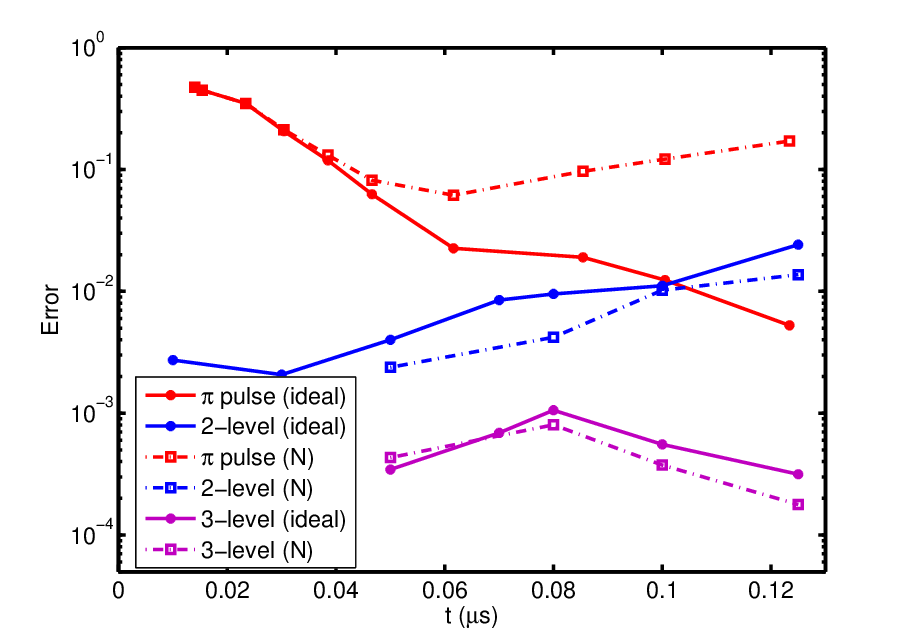
Ideal case: Next we show that the optimal control theory can achieve a CNOT gate with a better fidelity than simply applying a conditional pulse (CROT). The CNOT or CROT gate errors as a function of the gate operation time for different cases are illustrated in Fig. 3. The solid lines and dot-dashed lines represent the gate errors obtained for the ideal case and the case including noise qubit , respectively. The red lines represent the CROT gate errors obtained by applying a conditional pulse taking states of the NV center as the system qubit states. The blue lines and purple lines represent the CNOT gate errors obtained by using the optimal control theory taking the NV center electron spin as a two-level system and three-level system, respectively. Note that different from the gate error of the CROT implemented by a conditional pulse, the QOC gate errors are calculated by substituting the pulse sequence obtained in respective methods into the Hamiltonian of the three-level NV center system including the noise qubit (but not including the bath spins) for the propagator in Eq. (12). For the idea case (solid lines), when the gate operation time becomes shorter, the gate error using a pulse becomes larger. The reason is that the requirement for a shorter duration of a pulse means a stronger field strength, which in turn induces a larger transition probability to the leakage state. In contrast, the QOC theory can do a much better job when the operation time is short as illustrated in Fig.3. However, as the operation time increases, the error for the optimal control case of treating the electron spin as an effective two-level system becomes larger, even larger than that of using a pulse (see Fig.3). Therefore, employing QOC for the three-level electron spin system is necessary. It is quite obvious from Fig.3 that employing the QOC theory by treating the electron spin as a three-level system (purple solid lines) gives gate errors one order to two orders of magnitude lower than those of the two-level case (blue solid line).


.
Effect of a noise qubit: In the case of including the noise qubit, driving the system by a pulse does not work well anymore (see the red dot-dashed line). However, taking the noise qubit into the QOC optimization consideration lowers the error or infidelity a little bit as compared to the case without doing so. One can see this from Fig.3 that the blue and purple dot-dashed lines are slightly lower than their corresponding blue and purple solid lines, respectively. The reason is that the noise qubit here also serves as an ancilla qubit that allows some probability to get out of the computational space temporarily but return to the computational space with higher fidelity at the end of the operation for the optimal control CNOT gate. Again, treating the electron spin as a three-level system is a more effective strategy to perform CNOT gate and it gives an error in the presence of the noise qubit for a gate time of . Figure 4(a) investigates the optimal control CNOT gate error as a function of the strength of the external static magnetic field for a gate operation time of . The blue solid line and red dot-dashed line represent the cases of treating the electron spin as a two-level system and a three-level system, respectively. When the static magnetic field decreases, the gate error represented by the blue solid line becomes large. This is because at a lower magnetic field the energy separation between the qubit state and the leakage state become smaller, and thus the approximation of treating the NV electron spin as a two-level system of is not very good. However, the optimal control of the three-level case still works with error even when the magnetic field is as low as . The optimal control field sequences by treating the NV electron spin as a three-level system for G (red dot-dashed lines) and G (blue solid lines) with the operation time of are shown in Fig. 4(b). At (), the energy separation between the electron qubit states of and is much larger than (comparable to) the energy splitting between the states and (due to the hyperfine interaction), where and represent the nuclear spin states, and and represent the electron qubit states. As a result, there are apparently two different oscillating components for the case of G (blue solid lines) as compared to the case of (red dot-dashed lines) in Fig. 4(b). The major frequency of the fast oscillating component comes from the high frequency (energy separation) of the electron qubit, while that of the slow one matches the energy splitting between states and .

Effect of a spin bath: Next, we take into account not only the noise qubit but also the bath of the distant spin impurities, which is modeled as an effective classical random field acting on the NV electron spin with correlation function given by Eq. (6). The solid lines in Fig. 5 show the dependence of the CNOT gate error on the bath parameter for the correlation time . The parameter defined in the bath correlation function, Eq. (6), is related to the average system-bath coupling strength or field inhomogeneity in the random field model. The dashed lines in Fig. 5 represent the gate error obtained by applying the optimal control sequences obtained for the case without the spin bath to the master equation or the effective evolution equation (10) in the presence of the bath. This allows us to study how the gate errors due to the spin bath are improved in the open system by QOC. One can see from Fig. 5 that for unless the parameter is more than one order of magnitude larger than the typical value of extracted from the experiments [85, 40, 51], the influence of the bath on the gate with a short operation time of (blue dashed line) is not significant. For the longer gate operation time of red dashed line), the influence of a bath becomes appreciable when , and as the coupling strength become stronger, the error increases. However, the optimal control CNOT gate with operation time (blue solid line) can sustain much larger values of the field inhomogeneity up to and the gate error can be maintained almost the same as if the spin bath were not present.

The relation between the gate error and the bath correlation time for the average coupling strengths of and the operation time of ( and operation time ) is shown in red solid line (blue solid line) in Fig. 6. To investigate how much QOC theory improves the gate fidelity in the NV center system with a spin bath, we take the optimal pulse sequences in the absent of the spin bath as our initial guess for the control fields, and the gate errors before the optimal control iterations are shown in dot-dashed lines in Fig.6. The gate errors (solid lines) after the iterations are terminated are larger for small values of , and decrease as increases. The gate errors (solid lines) stay nearly constant as . When the bath correlation time is small, the memory effect of the bath is weak and the bath is close to a Markovian bath. In this case, it is hard to revise the bath contribution since the decay rate approaches to a steady value in a very short time. In contrast, when is large, due to the relatively long memory effect of the bath, the optimal control fields are able to counteract the influence from the bath.
VI CONCLUSION
We have found the control sequences of fast and high-fidelity single-qubit and two-qubit quantum gates for electron and nuclear spins of a NV center in diamond using the QOC theory. A CNOT gate or other general quantum gates operation can be implemented in a single run of pulse sequence using the optimal control approach rather than being decomposed into some entangled two-qubit and several single-qubit operations in series by composite pulse sequences. The (non-Markovian) external environment effects on system qubits are partitioned into two kinds, one from a few nearby noise qubits and the other from a bath of distant spins. Table 1 summarizes the gate time and gate errors calculated with realistic experimental parameters for the cases considering the effect of the noise qubits, the leakage state and the effect of a spin bath. These gate errors are below the recent model of error threshold [72] ( if surface code error correction is used [73, 74, 75]) required for FTQC. One can estimate the logical error rate that our gate error corresponds to for a given type of error correction of FTQC. Suppose that one implements a logical qubit of the surface code error correction on a two-dimensional array of physical qubits with array size (distance) [corresponding to the number of physical qubits being ] as in Ref. [75]. The number of physical qubits or the array size needed to define a logical qubit to meet a required logical error rate is dependent strongly on the error rate in the physical qubits. By taking the error probability per step to be the worse gate error of in Table 1, which is smaller than the error threshold rate of of the surface code, the estimated logical error rates using Fig. 4 or more precisely Eq. (11) of Ref. [75] are about for array size and about for array size . When the per-step error rate is smaller than the error threshold rate , the logical error rate falls exponentially with the array size . Thus one obtains the logical error rate for array size to be about , sufficient to perform Shor’s algorithm for factoring a -bit number into its primes with a reasonable chance of success [75].
There seems to be challenges for the experimental implementations and applications of the QOC theory, such as imprecise knowledge of the quantum system’s parameters and how to generate the complex optimal control pulses in reality. Fortunately, commercial devices for generating arbitrary wave forms or complex signals in a time scale of sub-nanoseconds to nanoseconds are available now and may solve the challenge of generating complex pulse sequences. Besides, a hybrid open-loop–closed-loop optimal control method called adaptation by hybrid optimal control (Ad-HOC) method [89] designed to overcome not only the problem of inaccurate knowledge of the system parameters but also shortcomings of the assumed physical model and errors on the control fields has been recently proposed. The closed-loop pulse calibration of Ad-HOC, similar to adaptive model-free feedback control (also referred to as closed-loop laboratory control or learning control) [90, 91], uses the physical system itself as a feedback to calibrate control pulses and optimize their performance. Two similar closed-loop methods for optimizing quantum control in experimental systems have also been put forward recently: the method of optimized randomized benchmarking for immediate tune-up (ORBIT) [92] and the method of adaptive control via randomized optimization nearly yielding maximization (ACRONYM) [93]. In principle, the system response and control pulses can be calibrated and improved using closed-loop optimization where measurement data are efficiently obtained with Nelder-Mead algorithm [89, 92, 94] or stochastic optimization algorithm [93, 95, 96] and subsequently fed back to the system optimizer to improve the pulses without precise knowledge of the system. These developments make the QOC theory practical and useful to construct the initial pulse sequences for experimentally closed-loop optimization [89].
Acknowledgements.
We acknowledge support from the the Ministry of Science and Technology of Taiwan under Grant No. 103-2112-M-002-003-MY3, from the National Taiwan University under Grants No. NTU-ERP-104R891402, and from the thematic group program of the National Center for Theoretical Sciences, Taiwan.Appendix A Explicit form of
Employing the algorithm of the Krotov optimization method, we evolve backward in time the auxiliary function with the boundary condition . Therefore, we need to find the explicit form of . The procedure and calculation presented below follows those in Ref. 82.
In our case, the error function is defined through Eqs. (12) and (13). The matrix elements of can be written as
| (15) |
where the matrix indices and range form to and is the matrix element (a complex scalar variable) of . Let , and be a matrix function of the variable , and be a scalar function. Thus, the error function (12) in terms of the new variables is . Note that is not an analytic function of but can be expressed as an analytic function of and . Consequently, when one differentiates with respect to , and subsequently are treated as constants. Thus
| (16) |
Here the second line in Eq. (16) follows from the use of the chain rule, and the last line follows from the property of . Then from the definition of and , we find that
| (17) |
Since , inserting the trace of Eq. (17) into Eq. (16), we finally obtain the explicit form of
| (18) |
where
| (19) |
can be simply obtained by the definition of in Eq. (13). Here and denote the smallest integers greater than or equal to and , respectively, and are the matrix elements of the target gate. In Eq. (19), the states are the elements of the orthonormal basis matrix of the noise qubit(s).
References
- [1] G. Balasubramanian, P. Neumann, D. Twitchen, M. Markham, R. Kolesov, N. Mizuochi, J. Isoya, J. Achard, J. Beck, J. Tissler, V. Jacques, P. R. Hemmer, F. Jelezko, and J. Wrachtrup, Nat. Mater. 8, 383 (2009).
- [2] A. Jarmola, V. M. Acosta, K. Jensen, S. Chemerisov, and D. Budker, Phys. Rev. Lett. 108, 197601 (2012).
- [3] T. Ishikawa, K.-M. C. Fu, C. Santori, V. M. Acosta, R. G. Beausoleil, H.Watanabe, S. Shikata, and K. M. Itoh, Nano Lett. 12, 2083 (2012).
- [4] K. Fang, V. M. Acosta, C. Santori, Z. Huang, K. M. Itoh, H. Watanabe, S. Shikata, and R. G. Beausoleil, Phys. Rev. Lett. 110, 130802 (2013).
- [5] N. Bar-Gill, L. M. Pham, A. Jarmola, D. Budker, and R. L. Walsworth, Nat. Commun. 4, 1743 (2013).
- [6] P. C. Maurer, G. Kucsko, C. Latta, L. Jiang, N. Y. Yao, S. D. Bennett, F. Pastawsk, D. Hunger, N. Chisholm, M. Markham, D. J. Twitchen, J. I. Cirac, and M. D. Lukin, Science 336, 1283 (2012).
- [7] F. Jelezko, I. Popa, A. Gruber, C. Tietz, J. Wrachtrup, A. Nizovtsev and S. Kilin, Appl. Phys. Lett. 81, 2160 (2002).
- [8] F. Jelezko, T. Gaebel, I. Popa, A. Gruber, and J. Wrachtrup, Phys. Rev. Lett. 92, 076401 (2004).
- [9] R. J. Epstein, F. M. Mendoza, Y. K. Kato and D. D. Awschalom, Nature Phys. 1, 94 (2005).
- [10] G. Balasubramanian, I. Y. Chan, R. Kolesov, M. Al-Hmoud, J. Tisler, C. Shin, C. Kim, A.Wojcik, P. R. Hemmer, A. Krueger, T. Hanke, A. Leitenstorfer, R. Bratschitsch, F. Jelezko, and J. Wrachtrup, Nature (London) 455, 648 (2008).
- [11] J. R. Maze, P. L. Stanwix, J. S. Hodges, S. Hong, J. M. Taylor, P. Cappellaro, L. Jiang, M. V. G. Dutt, E. Togan, A. S. Zibrov, A. Yacoby, R. L.Walsworth, andM. D. Lukin, Nature (London) 455, 644 (2008).
- [12] V. M. Acosta, E. Bauch, M. P. Ledbetter, C. Santori, K. M. C. Fu, P. E. Barclay, R. G. Beausoleil, H. Linget, J. F. Roch, F. Treussart, S. Chemerisov, W. Gawlik, and D. Budker, Phys. Rev. B 80, 115202 (2009).
- [13] S., Kolkowitz, Q. P., Unterreithmeier, S. D., Bennett, and M. D., Lukin, Phys. Rev. Lett. 109, 137601 (2012).
- [14] T. H. Taminiau, J. J. T. Wagenaar, T. van der Sar, F. Jelezko, V. V. Dobrovitski, and R. Hanson, Phys. Rev. Lett. 109, 137602 (2012).
- [15] Zhao, N. et al. N. Zhao, J. Honert, B. Schmid, J. Isoya, M. Markham, D. Twitchen, F. Jelezko, R.-B. Liu, H. Fedder et al., Nat. Nanotechnol. 7, 657 (2012).
- [16] T. Staudacher, F. Shi, S. Pezzagna, J. Meijer, J. Du, C. A. Meriles, F. Reinhard and J. Wrachtrup, Science 339, 561 (2013).
- [17] H. J. Mamin, M. Kim, M. H. Sherwood, C. T. Rettner, K. Ohno, D. D. Awschalom and D. Rugar, Science 339, 557 (2013).
- [18] P. Maletinsky, S. Hong, M. S. Grinolds, B. Hausmann, M. D. Lukin, R. L. Walsworth, M. Loncar and A. Yacoby, Nat. Nanotechnol. 7, 320 (2012).
- [19] M. Loretz, T. Rosskopf, and C. L. Degen, Phys. Rev. Lett. 110, 017602 (2013).
- [20] J. Cai, F. Jelezko, and M. B. Plenio, Nat. Commun. 5, 4065 (2014).
- [21] P. H. Chung, E. Perevedentseva, J. S. Tu, C. C. Chang, and C. L. Cheng, Diamond Relat. Mater. 15, 622 (2006).
- [22] C.-C. Fu, H.-Y. Lee, K. Chen, T.-S. Lim, H.-Y. Wu, P.-K. Lin, P.-K. Wei, P.-H. Tsao, H.-C. Chang, and W. Fann, Proc. Natl. Acad. Sci. USA 104, 727 (2007).
- [23] J.-I. Chao, E. Perevedentseva, P.-H. Chung, K.-K. Liu, C.-Y. Cheng, C.-C. Chang, and C.-L. Cheng, Biophys. J. 93, 2199 (2007).
- [24] F. Neugart, A. Zappe, F. Jelezko, C. Tietz, J. P. Boudou, A. Krueger, and J. Wrachtrup, Nano Lett. 7, 3588 (2007).
- [25] A. Beveratos, S. Kühn, R. Brouri, T. Gacoin, J.-P. Poizat, and P. Grangier, Eur. Phys. J. D 18, 191 (2002).
- [26] A. Beveratos, R. Brouri, T. Gacoin, A. Villing, J. P. Poizat, and P. Grangier, Phys. Rev. Lett. 89, 187901 (2002).
- [27] F. Jelezko, T. Gaebel, I. Popa, M. Domhan, A. Gruber, and J. Wrachtrup, Phys. Rev. Lett. 93, 130501 (2004).
- [28] L. I. Childress, J. M. Taylor, A. S. Sørensen, and M. D. Lukin, Phys. Rev. A 72, 052330 (2005).
- [29] L. Childress, J. M. Taylor, A. S. Sørensen, and M. D. Lukin, Phys. Rev. Lett. 96, 070504 (2006).
- [30] L. Jiang, J. M. Taylor, A. S. Sørensen, and M. D. Lukin, Phys. Rev. A 76, 062323 (2007).
- [31] S. D. Barrett and P. Kok, Phys. Rev. A 71, 060310 (2005).
- [32] M. V. Gurudev Dutt, L. Childress, L. Jiang, E. Togan, J. Maze, F. Jelezko, A. S. Zibrov, P. R. Hemmer, M. D. Lukin, Science 316, 1312 (2007).
- [33] P. Neumann, N. Mizuochi, F. Rempp, P. Hemmer, H. Watanabe, S. Yamasaki, V. Jacques, T. Gaebel, F. Jelezko and J. Wrachtrup, Science 320, 1326 (2008).
- [34] G. D. Fuchs, V. V. Dobrovitski, D. M. Toyli, F. J. Heremans and D. D. Awschalom, Science 326, 1520 (2009).
- [35] P. Cappellaro, L. Jiang, J. S. Hodges, and M. D. Lukin, Phys. Rev. Lett. 102, 210502 (2009).
- [36] P. Neumann, R. Kolesov, B. Naydenov, J. Beck, F. Rempp, M. Steiner, V. Jacques, G. Balasubramanian, M. L. Markham et al., Nat. Phys. 6, 249 (2010).
- [37] F. Shi, X. Rong, N. Xu, Y. Wang, J. Wu, B. Chong, X. Peng, J. Kniepert, R. S. Schoenfeld, W. Harneit, M. Feng, and J. F. Du, Phys. Rev. Lett. 105, 040504 (2010).
- [38] G. D. Fuchs, G. Burkard, P. V. Klimov, and D. D. Awschalom, Nat. Phys. 7, 789 (2011).
- [39] X. K. Xu, Z. X. Wang, C. K. Duan, P. Huang, P. F. Wang, Y. Wang, N. Y. Xu, X. Kong, F. Z. Shi, X. Rong, and J. F. Du, Phys. Rev. Lett. 109, 070502 (2012).
- [40] T. van der Sar, Z. H. Wang, M. S. Blok, H. Bernien, T. H. Taminiau, D. M. Toyli, D. A. Lidar, D. D. Awschalom, R. Hanson, and V. V. Dobrovitski, Nature (London) 484, 82 (2012).
- [41] G.-Q. Liu, H. C. Po, J. Du, R.-B. Liu, and X.-Y. Pan, Nat. Commun. 4, 2254 (2013).
- [42] J. H. Shim, I. Niemeyer, J. Zhang, and D. Suter, Phys. Rev. A 87, 012301 (2013).
- [43] F. Dolde, I. Jakobi, B. Naydenov, N. Zhao, S. Pezzagna, C. Trautmann, J. Meijer, P. Neumann, F. Jelezko, and J. Wrachtrup, Nature Phys. 9, 139 (2013).
- [44] J. Zhang, A. M. Souza, F. D. Brandao, and D. Suter, Phys. Rev. Lett. 112, 050502 (2014).
- [45] X. Rong, J. Geng, Z. Wang, Q. Zhang, C. Ju, F. Shi, C.-K. Duan, and J. Du, Phys. Rev. Lett. 112, 050503 (2014).
- [46] T. H. Taminiau, J. Cramer, T. van der Sar, V. V. Dobrovitski and R. Hanson, Nat. Nanotechnolo. 9, 171 (2014).
- [47] G. Waldherr, Y. Wang, S. Zaiser, M. Jamali, T. Schulte-Herbrüggen , H. Abe, T. Oshima, J. Isoya, J. F. Du, P. Neumann, and J. Wrachtrup, Nature (London) 506, 204 (2014).
- [48] F. Dolde, V. Bergholm, Y. Wang, I. Jakobi, S. Pezzagna, J. Meijer, P. Neumann, T. Schulte-Herbrüggen J. Biamonte, and J. Wrachtrup, Nat. Commun. 5, 3371 (2014).
- [49] J. Scheuer, X. Kong, R. S. Said, J. Chen, A. Kurz, L. Marseglia, J. Du, P. R. Hemmer, S. Montangero, T. Calarco, B. Naydenov, and F. Jelezko, New J. Phys. 16, 093022 (2014)
- [50] B. Scharfenberger, W. J Munro, and K. Nemoto, New J. Phys. 16 093043 (2014).
- [51] G. de Lange, Z. H. Wang, D. Ristè, V. V. Dobrovitski, and R. Hanson, Science 330, 60 (2010) .
- [52] Z.-H. Wang, G. de Lange, D. Riste, R. Hanson, and V. V. Dobrovitski, Phys. Rev. B 85, 155204 (2012).
- [53] N. Zhao, S.-W. Ho, and R.-B. Liu, Phys. Rev. B 85, 115303 (2012).
- [54] A. P. Peirce, M. A. Dahleh, and H. Rabitz, Phys. Rev. A 37, 4950 (1988).
- [55] D. J. Tannor, V. A. Kazakov and V. Orlov, in Time-Dependent Quantum Molecular Dynamics, edited by J. Broeckhove and L. Lathouwers, NATO Advanced Studies Institute, Series B: Physics (Plenum Press, New York, 1992), Vol. 299, pp. 347-360.
- [56] J. P. Palao and R. Kosloff, Phys. Rev. Lett. 89, 188301 (2002); J. P. Palao and R. Kosloff, Phys. Rev. A 68, 062308 (2003).
- [57] S. E. Sklarz and D. J. Tannor, Phys. Rev. A 66, 053619 (2002).
- [58] R. Xu, Y. Yan, Y. Ohtsuki, Y. Fujimura, and H. Rabitz, J. Chem. Phys. 120, 6600 (2004).
- [59] N. Khaneja, T. Reiss, C. Kehlet, T. Schulte-Herbrüggen, and S. J. Glaser, J. Magn. Reson. 172, 296 (2005).
- [60] A. Spörl, T. Schulte-Herbrüggen, S. J. Glaser, V. Bergholm, M. J. Storcz, J. Ferber, and F. K. Wilhelm, Phys. Rev. A 75, 012302 (2007).
- [61] D.-B. Tsai, P.-W. Chen, and H.-S. Goan, Phys. Rev. A 79, 060306(R) (2009).
- [62] R. Eitan, M. Mundt, and D. J. Tannor, Phys. Rev. A 83, 053426 (2011).
- [63] S. Montangero, T. Calarco, and R. Fazio, Phys. Rev. Lett. 99, 170501 (2007).
- [64] I. I. Maximov, Z. Tošner, and N. C. Nielsen, J. Chem. Phys. 128, 184505 (2008).
- [65] M. Wenin and W. Pötz, Phys. Rev. A 78, 012358 (2008); M. Wenin and W. Pötz, Phys. Rev. B 78, 165118 (2008); M. Wenin, R. Roloff, and W. Pötz, J. Appl. Phys. 105, 084504 (2009).
- [66] R. Roloff and W. Pötz, Phys. Rev. B 79, 224516 (2009); M. Wenin and W. Pötz, Phys. Rev. A 74, 022319 (2006).
- [67] H. Jirari, Europhys. Lett. 87, 40003 (2009).
- [68] P. Rebentrost, I. Serban, T. Schulte-Herbrüggen, and F. K. Wilhelm, Phys. Rev. Lett. 102, 090401 (2009).
- [69] B. Hwang and H.-S. Goan, Phys. Rev. A 85, 032321 (2012).
- [70] J.-S. Tai, K.-T. Lin and H.-S. Goan, Phys. Rev. A 89, 062310 (2014).
- [71] S.-Y. Huang and H.-S. Goan, Phys. Rev. A 90, 012318 (2014).
- [72] P. Aliferis and J. Preskill, Phys. Rev. A 79, 012332 (2009).
- [73] D. S. Wang, A. G. Fowler, and L. C. L. Hollenberg, Phys. Rev. A 83, 020302(R) (2011).
- [74] A. G. Fowler, A. C. Whiteside, and L. C. L. Hollenberg, Phys. Rev. Lett. 108, 180501 (2012),
- [75] A. G. Fowler, M. Mariantoni, J. M. Martinis, A. N. Cleland, Phys. Rev. A 86, 032324 (2012)
- [76] V. F. Krotov, Global Methods in Optimal Control Theory (Marcel Dekker, New York, 1996).
- [77] F. Reinhard, F. Shi, N. Zhao, F. Rempp, B. Naydenov, J. Meijer, L. T. Hall, L. Hollenberg, J. Du, R.-B. Liu, and J. Wrachtrup, Phys. Rev. Lett. 108, 200402 (2012)
- [78] J. R. Rabeau, P. Reichart, G. Tamanyan, D. N. Jamieson, S. Prawer, F. Jelezko, T. Gaebel, I. Popa, M. Domhan and J. Wrachtrup, Appl. Phys. Lett. 88, 023113 (2006).
- [79] Z.-H. Wang and S. Takahashi, Phys. Rev. B 87, 115122 (2013).
- [80] J.-M. Cai, B. Naydenov, R. Pfeiffer, L. P. McGuinness, K. D. Jahnke, F. Jelezko, M. B. Plenio, and A. Retzker, New J. Phys. 14, 113023 (2012).
- [81] A. Bermudez, F. Jelezko, M. B. Plenio, and A. Retzker, Phys. Rev. Lett. 107, 150503 (2011).
- [82] M. D. Grace, C. Brif, H. Rabitz, I. A. Walmsley, R. L. Kosut, and D. A. Lidar, J. Phys. B: At. Mol. Opt. Phys. 40, S103 (2007a).
- [83] M. D. Grace, C. Brif, H. Rabitz, D. A. Lidar, I. A. Walmsley, and R. L. Kosut, J. Mod. Opt. 54, 2339 (2007b).
- [84] H.-S. Goan, C.-C. Jian, and P.-W. Chen, Phys. Rev. A 82, 012111 (2010).
- [85] R. Sousa, in Electron Spin Resonance and Related Phenomena in Low-Dimensional Structures, Topics in Applied Physics, Vol. 115, edited by M. Fanciulli (Springer Berlin, 2009) pp. 183–220.
- [86] S. Welack, M. Schreiber, and U. Kleinekathofer, J. Chem. Phys. 124, 044712 (2006).
- [87] U. Kleinekathofer, J. Chem. Phys. 121, 2505 (2004).
- [88] M. D. Grace, J. Dominy, R. L. Kosut, C. Brif, and H. Rabitz, New J. Phys. 12, 015001 (2010).
- [89] D. J. Egger and F. K. Wilhelm, Phys. Rev. Lett. 112, 240503 (2014).
- [90] R. S. Judson and H. Rabitz, Phys. Rev. Lett. 68, 1500 (1992).
- [91] C. Brif, R. Chakrabarti, and H. Rabitz, New J. Phys. 12, 075008 (2010).
- [92] J. Kelly et al., Phys. Rev. Lett. 112, 240504 (2014).
- [93] C. Ferrie and O. Moussa, arXiv:1409.3172.
- [94] J. A. Nelder and R. Mead, Comput. J. 7, 308 (1965).
- [95] J. C. Spall, IEEE Trans. Automat. Contr. 37, 332 (1992).
- [96] J. C. Spall, Introduction to Stochastic Search and Optimization: Estimation, Simulation, and Control (John Wiley & Sons, Hoboken, NJ, 2005).