跳到论文正文
W Papers独立论文阅读器 arXiv:1504.06280 论文正文 计算阅读时间 · 0%
引用这篇论文根据当前论文元数据生成,正式投稿前建议核对。


License: arXiv.org perpetual non-exclusive license
arXiv:1504.06280v2 [math.PR] 15 Apr 2016

Excited random walks with Markovian cookie stacksThanks: E. Kosygina was partially supported by the Simons Foundation through a Collaboration Grant for Mathematicians #209493 and Simons Fellowship in Mathematics, 2014-2015. She also thanks Institut Mittag-Leffler for support and stimulating research environment.Thanks: J. Peterson was partially supported by NSA grant H98230-13-1-0266.

Elena Kosygina Address: Elena Kosygina
One Bernard Baruch Way
Department of Mathematics, Box B6-230
Baruch College
New York, NY 10010
USA
Email address: elena.kosygina@baruch.cuny.edu URL: www.baruch.cuny.edu/math/facultystaff/ekosygina/kosygina.html
and Jonathon Peterson Address: Jonathon Peterson
Purdue University
Department of Mathematics
150 N University Street
West Lafayette, IN 47907
USA
Email address: peterson@purdue.edu URL: www.math.purdue.edu/˜peterson
Abstract.

We consider a nearest-neighbor random walk on ℤ\mathbb{Z} whose probability ωx​(j)\omega_{x}(j) to jump to the right from site xx depends not only on xx but also on the number of prior visits jj to xx. The collection (ωx​(j))x∈ℤ,j≥1(\omega_{x}(j))_{x\in\mathbb{Z},j\geq 1} is sometimes called the “cookie environment” due to the following informal interpretation. Upon each visit to a site the walker eats a cookie from the cookie stack at that site and chooses the transition probabilities according to the “strength” of the cookie eaten. We assume that the cookie stacks are i.i.d. and that the cookie “strengths” within the stack (ωx​(j))j≥1(\omega_{x}(j))_{j\geq 1} at site xx follow a finite state Markov chain. Thus, the environment at each site is dynamic, but it evolves according to the local time of the walk at each site rather than the original random walk time.

The model admits two different regimes, critical or non-critical, depending on whether the expected probability to jump to the right (or left) under the invariant measure for the Markov chain is equal to 1/21/2 or not. We show that in the non-critical regime the walk is always transient, has non-zero linear speed, and satisfies the classical central limit theorem. The critical regime allows for a much more diverse behavior. We give necessary and sufficient conditions for recurrence/transience and ballisticity of the walk in the critical regime as well as a complete characterization of limit laws under the averaged measure in the transient case.

The setting considered in this paper generalizes the previously studied model with periodic cookie stacks [KOS14]. Our results on ballisticity and limit theorems are new even for the periodic model.

Key words and phrases: 
Excited random walk, diffusion approximation, stable limit laws, random environment, branching-like processes
2010 Mathematics Subject Classification
Primary 60K37; Secondary 60F05, 60J10, 60J15, 60K35

1. Introduction

Excited random walks (ERWs, also called cookie random walks) are a model for a self-interacting random motion where the self-interaction is such that the transition probabilities for the next step of the random walk depend on the local time at the current location. To make this precise, a cookie environment ω={ωx​(j)}x∈ℤ,j≥1\omega=\{\omega_{x}(j)\}_{x\in\mathbb{Z},\,j\geq 1} is an element of Ω=[0,1]ℤ×ℕ\Omega=[0,1]^{\mathbb{Z}\times\mathbb{N}}, and given a cookie environment ω∈Ω\omega\in\Omega and x∈ℤx\in\mathbb{Z}, the ERW in the cookie environment ω\omega started at xx is a stochastic process {Xn}n≥0\{X_{n}\}_{n\geq 0} with law PωxP_{\omega}^{x} such that Pωx​(X0=x)=1P_{\omega}^{x}(X_{0}=x)=1 and

Pωx​(Xn+1=Xn+1|X0,X1,…,Xn)\displaystyle P_{\omega}^{x}\left(X_{n+1}=X_{n}+1\,|\,X_{0},X_{1},\dots,X_{n}\right) =1−Pωx​(Xn+1=Xn−1|X0,X1,…,Xn)\displaystyle=1-P_{\omega}^{x}\left(X_{n+1}=X_{n}-1\,|\,X_{0},X_{1},\dots,X_{n}\right)
=ωXn​(#⁡{k≤n:Xk=Xn}).\displaystyle=\omega_{X_{n}}(\#\{k\leq n:\,X_{k}=X_{n}\}).

The “cookie” terminology in the above description of ERWs comes from the following interpretation. One imagines a stack of cookies at each site x∈ℤx\in\mathbb{Z}. Upon the jj-th visit to the site xx the random walker eats the jj-th cookie at that site which induces a step to the right with probability ωx​(j)\omega_{x}(j) and to the left with probability 1−ωx​(j)1-\omega_{x}(j). For this reason we will refer to ωx​(j)\omega_{x}(j) as the strength of the jj-th cookie at site xx.

Many results for ERWs in one dimension were obtained under the assumption that there is an M<∞M<\infty such that ωx​(j)=1/2\omega_{x}(j)=1/2 for all j>Mj>M and x∈ℤx\in\mathbb{Z} [BW03, MPV06, BS08a, BS08b, KZ08, KM11, DK12, Pet12, Pet13, AO16, Pet15]. We will refer to this as the case of “boundedly many cookies per site”. Much less is known if the number of cookies per site is not bounded (in particular, if there are infinitely many cookies at each site). Notable exceptions are that Zerner [Zer05] proved a criterion for recurrence/transience and Dolgopyat [Dol11] proved the scaling limits for the recurrent case under the assumption that ωx​(j)≥1/2\omega_{x}(j)\geq 1/2 for all x∈ℤx\in\mathbb{Z} and j≥1j\geq 1 (i.e., all cookies have non-negative drift). For a review (prior to 2012) of ERWs in one and more dimensions see [KZ13].

Until recently, very little was known for ERWs which had infinitely many cookies per site with both positive and negative drift cookies.11 1 With the exception of one-dimensional random walk in random environment which can be seen as a particular case of ERW where ωx​(j)=ωx​(1)\omega_{x}(j)=\omega_{x}(1) for all j≥1j\geq 1 at each x∈ℤx\in\mathbb{Z}. However, [KOS14] gave an explicit criterion for recurrence/transience of ERWs in cookie environments such that the cookie sequence {ωx​(j)}j≥1\{\omega_{x}(j)\}_{j\geq 1} is the same for all xx and is periodic in jj. The results in the current paper cover more general cookie environments where the cookie stack at each site is given by a finite state Markov chain. Moreover, we add to the results of [KOS14] by also proving a criterion for ballisticity (non-zero limiting velocity) and limiting distributions in the transient case. We also note that our model is general enough to include the case of periodic cookie stacks as in [KOS14] as well as some cases of boundedly many cookies per site.

1.1. Description of the model

Let ℛ={1,2,…,N}\mathcal{R}=\{1,2,\ldots,N\} denote a finite state space, and let {Rj}j≥1\{R_{j}\}_{j\geq 1} be a Markov chain on ℛ\mathcal{R} with transition probabilities given by an N×NN\times N matrix K=(Ki,i′)i,i′∈ℛK=(K_{i,i^{\prime}})_{i,i^{\prime}\in\mathcal{R}}. We will assume that this Markov chain has a unique closed irreducible subset ℛ0⊆ℛ\mathcal{R}_{0}\subseteq\mathcal{R}. Thus, there is a unique stationary distribution μ\mu for the Markov chain {Rj}j≥1\{R_{j}\}_{j\geq 1}, and μ\mu is supported on ℛ0{\cal R}_{0}. Throughout the paper we will often represent probability distributions η\eta on ℛ\mathcal{R} as row vectors η=(η⁡(1),η⁡(2),…,η⁡(N))\eta=(\eta(1),\eta(2),\ldots,\eta(N)), so that for the stationary distribution μ\mu we have μ​K=μ\mu K=\mu.

Assumptions (i.i.d., elliptic, Markovian cookie stacks).

Let {𝐑x}x∈ℤ\{\mathbf{R}^{x}\}_{x\in\mathbb{Z}} be an i.i.d. family of Markov chains 𝐑x={Rjx}j≥1\mathbf{R}^{x}=\{R_{j}^{x}\}_{j\geq 1} with transition matrix KK. We assume that the cookie environment ω\omega is given by ωx​(j)=p⁡(Rjx)\omega_{x}(j)=p(R_{j}^{x}) for some fixed function p:ℛ→(0,1)p:\mathcal{R}\rightarrow(0,1). The requirement that pp is strictly between 00 and 11 will be referred to as ellipticity throughout the paper.

For any distribution η\eta on ℛ\mathcal{R}, let ℙη\mathbb{P}_{\eta} denote the distribution of {Rjx}x∈ℤ,j≥1\{R^{x}_{j}\}_{x\in\mathbb{Z},j\geq 1} when each R1xR_{1}^{x}, x∈ℤx\in\mathbb{Z}, has distribution η\eta. With a slight abuse of notation ℙη\mathbb{P}_{\eta} will also be used for the induced distribution on environments ω\omega which is constructed as in the assumptions above. If η\eta is concentrated on a single state i∈ℛi\in{\cal R}, i.e. if η=δi\eta=\delta_{i}, we shall use ℙi\mathbb{P}_{i} instead of ℙδi\mathbb{P}_{\delta_{i}}. Expectations with respect to ℙη\mathbb{P}_{\eta} or ℙi\mathbb{P}_{i} will be denoted by 𝔼η\mathbb{E}_{\eta} and 𝔼i\mathbb{E}_{i}, respectively.

As stated above, the law of the ERW in a fixed cookie environment ω\omega is denoted PωxP_{\omega}^{x}. We will refer to this as the quenched law. If the cookie environment has distribution ℙη\mathbb{P}_{\eta}, then we can also define the averaged law of the ERW by Pηx​(⋅)=𝔼η​[Pωx​(⋅)]P_{\eta}^{x}(\cdot)=\mathbb{E}_{\eta}[P_{\omega}^{x}(\cdot)]. Expectations with respect to the quenched and averaged measures will be denoted by EωxE_{\omega}^{x} and EηxE_{\eta}^{x}, respectively. Again, if η\eta is concentrated on i∈ℛi\in\mathcal{R} we shall set Pix​(⋅):=𝔼i​[Pωx​(⋅)]P_{i}^{x}(\cdot):=\mathbb{E}_{i}[P_{\omega}^{x}(\cdot)]. We will often be interested only in ERWs started at X0=0X_{0}=0, and so we will use the notation PωP_{\omega}, PηP_{\eta}, or PiP_{i} in place of Pω0P_{\omega}^{0}, Pη0P_{\eta}^{0} or Pi0P_{i}^{0}, respectively.

Example 1.1 (Periodic cookie sequences).

The model above clearly generalizes the case of periodic cookie sequences at each site as in [KOS14]. To obtain periodic cookie sequences set Ki,i+1=1K_{i,i+1}=1 for i=1,…,N−1i=1,\ldots,N-1, KN,1=1K_{N,1}=1, and let η=δ1\eta=\delta_{1}.

Example 1.2 (Cookies stacks of geometric height).

Fix α∈(0,1]\alpha\in(0,1], p⁡(1)>1/2p(1)>1/2, and p⁡(2)=1/2p(2)=1/2. Let K=(1−αα01)K=\begin{pmatrix}1-\alpha&\alpha\\ 0&1\end{pmatrix}. If η=δ1\eta=\delta_{1} then the cookie environment is such that there are an i.i.d. Geometric(α\alpha) number of cookies of strength p⁡(1)>1/2p(1)>1/2 at each site.

Example 1.3 (Bounded cookie stacks).

The model above also generalizes the case of finitely many cookies per site. For instance, let the transition matrix KK be such that Ki,i+1=1K_{i,i+1}=1 for i=1,…,N−1i=1,\ldots,N-1 and KN,N=1K_{N,N}=1, and let the function p:ℛ→(0,1)p:\mathcal{R}\rightarrow(0,1) be such that p⁡(N)=1/2p(N)=1/2. In this case, if η=δ1\eta=\delta_{1} then ωx​(j)=p​(j)\omega_{x}(j)=p(j) if j≤N−1j\leq N-1 and p⁡(j)=1/2p(j)=1/2 if j≥Nj\geq N. With a little more thought, one can also obtain random cookie environments that are i.i.d. spatially with a bounded number of cookies at each site as in [KZ08] subject to the restrictions that there are only finitely many possible values for the cookie strengths ωx​(j)\omega_{x}(j) and that ωx​(j)∈(0,1)\omega_{x}(j)\in(0,1). For instance, if

K=(0100000001000100000100001),𝐩=(p⁡(1)p⁡(2)p⁡(3)p⁡(4)1/2),andη=(α,0,1−α,0,0),K=\begin{pmatrix}0&1&0&0&0\\ 0&0&0&0&1\\ 0&0&0&1&0\\ 0&0&0&0&1\\ 0&0&0&0&1\end{pmatrix},\quad\mathbf{p}=\begin{pmatrix}p(1)\\ p(2)\\ p(3)\\ p(4)\\ 1/2\end{pmatrix},\quad\text{and}\quad\eta=(\alpha,0,1-\alpha,0,0),

then the corresponding cookie environments under the distribution ℙη\mathbb{P}_{\eta} have 2 cookies at each site, having stack (p⁡(1),p⁡(2))(p(1),p(2)) with probability α\alpha and stack (p⁡(3),p⁡(4))(p(3),p(4)) with probability 1−α1-\alpha.

Before stating our main results, we note two basic facts for ERWs that are known to hold in much more generality than our model. We will use these facts as needed throughout the paper.

Theorem 1.4 ([ABO16, Theorem 1.2] and [KZ13, Theorem 4.1]).
  1. (i)

    Zero-one law for transience. For any initial distribution η\eta on ℛ{\cal R}

    Pη​(limn→∞Xn=∞),Pη​(limn→∞Xn=−∞)∈{0,1}.P_{\eta}\left(\lim_{n\to\infty}X_{n}=\infty\right),\ P_{\eta}\left(\lim_{n\to\infty}X_{n}=-\infty\right)\in\{0,1\}.
  2. (ii)

    Strong law of large numbers: For any initial distribution η\eta on ℛ{\cal R} there is a deterministic v0∈[−1,1]v_{0}\in[-1,1] such that

    Pη​(limn→∞Xn/n=v0)=1.P_{\eta}\left(\lim_{n\to\infty}X_{n}/n=v_{0}\right)=1.

1.2. Main results

The function p:ℛ→(0,1)p:\mathcal{R}\rightarrow(0,1) used in the construction of the cookie environment ω\omega corresponds to a column vector 𝐩=(p⁡(1),p⁡(2),…,p⁡(N))t\mathbf{p}=(p(1),p(2),\ldots,p(N))^{t} with ii-th entry given by p⁡(i)p(i). Note that our assumptions on the Markov chains {𝐑x}x∈ℤ\{\mathbf{R}^{x}\}_{x\in\mathbb{Z}}, imply that the limiting average cookie strength at each site is

limk→∞1k​∑j=1kωx​(j)=μ⋅𝐩=:p¯,\lim_{k\rightarrow\infty}\frac{1}{k}\sum_{j=1}^{k}\omega_{x}(j)=\mu\cdot\mathbf{p}=:\bar{p},

and that this limit does not depend on the distribution η\eta of ωx​(1)\omega_{x}(1). It is natural to suspect that the ERW is transient to the right (resp. left) when p¯>1/2\bar{p}>1/2 (resp. p¯<1/2\bar{p}<1/2). Our first main result below confirms this is the case. Moreover, we also establish that if p¯≠1/2\bar{p}\neq 1/2 the walk has non-zero linear speed and a Gaussian limiting distribution.

Theorem 1.5.

Assume that p¯≠1/2\bar{p}\neq 1/2.

Transience:

If p¯>1/2\bar{p}>1/2 then Pη​(limn→∞Xn=∞)=1P_{\eta}(\lim_{n\rightarrow\infty}X_{n}=\infty)=1 for any initial distribution η\eta on ℛ\mathcal{R}. Similarly, if p¯<1/2\bar{p}<1/2 then Pη​(limn→∞Xn=−∞)=1P_{\eta}(\lim_{n\rightarrow\infty}X_{n}=-\infty)=1 for any η\eta.

Ballisticity:

For any initial distribution η\eta on ℛ\mathcal{R} the limiting velocity v0v_{0} (see Theorem 1.4(ii)) is non-zero: it is positive for p¯>1/2\bar{p}>1/2 and negative for p¯<1/2\bar{p}<1/2.

Gaussian limit:

For any distribution η\eta on ℛ\mathcal{R} there exists a constant b=b⁡(K,𝐩,η)>0b=b(K,\mathbf{p},\eta)>0 such that

limn→∞Pη(Xn−n​v0b​n≤x)=Φ(x):=∫−∞x12​πe−z2/2dz.\lim_{n\rightarrow\infty}P_{\eta}\left(\frac{X_{n}-nv_{0}}{b\sqrt{n}}\leq x\right)=\Phi(x):=\int_{-\infty}^{x}\frac{1}{\sqrt{2\pi}}e^{-z^{2}/2}\,dz.

The case p¯=1/2\bar{p}=1/2 is more interesting (we will refer to this as the critical case). In fact, it will follow from our results below that ERWs in the critical case p¯=1/2\bar{p}=1/2 can exhibit the full range of behaviors that are known for ERWs with boundedly many cookies per site (e.g., transience with sublinear speed and non-Gaussian limiting distributions). Before stating our results for the critical case, we remark that in the case of boundedly many cookies per site the classification of the long term behavior of the ERW is based on a single parameter δ=𝔼η​[∑j≥1(2​ωx​(j)−1)]\delta=\mathbb{E}_{\eta}[\sum_{j\geq 1}(2\omega_{x}(j)-1)] which is the expected total drift contained in a cookie stack. Our results below depend on two parameters δ\delta and δ~\tilde{\delta} which are also explicit but do not admit such simple interpretation. However, if we denote by ℰ0n{\cal E}^{n}_{0} the number of upcrossings (steps to the right) the ERW makes from 00 before the nn-th downcrossing (step to the left) from 00 then

δ=δ(η,K,𝐩):=2​ρν,where ρ:=limn→∞(𝔼η[ℰ0n]−n),andν:=limn→∞Varη​(ℰ0n)n.\delta=\delta(\eta,K,\mathbf{p}):=\frac{2\rho}{\nu},\quad\text{where }\rho:=\lim\limits_{n\to\infty}(\mathbb{E}_{\eta}[{\cal E}^{n}_{0}]-n),\quad\text{and}\quad\nu:=\lim\limits_{n\to\infty}\frac{\mathrm{Var}_{\eta}({\cal E}^{n}_{0})}{n}.

The parameter δ~\tilde{\delta} is defined in a symmetric way using downcrossings instead of upcrossings and vice versa so that δ~:=δ⁡(η,K,𝟏−𝐩)\tilde{\delta}:=\delta(\eta,K,\mathbf{1}-\mathbf{p}). The explicit formulas for the parameters are not intuitive and are given in (37) and (38). In the special case of boundedly many cookies per site the parameter δ\delta agrees with the one used in previous papers, δ~=−δ\tilde{\delta}=-\delta, and ν=2\nu=2. Proposition 4.3 below shows that in general δ+δ~=1−2/ν\delta+\tilde{\delta}=1-2/\nu where ν\nu need not be equal to 22 (see Example 1.13), and so two parameters are needed in the general model.

Theorem 1.6.

Fix an arbitrary initial distribution η\eta on ℛ{\cal R} and let p¯=μ⋅𝐩=1/2\bar{p}=\mu\cdot\mathbf{p}=1/2. Then, there exist constants δ\delta and δ~\tilde{\delta} satisfying δ+δ~<1\delta+\tilde{\delta}<1 (see (37) and (38) for the explicit formulas in terms of η\eta, KK, and 𝐩\mathbf{p}) and such that

  • •

    if δ>1\delta>1, then Pη​(limn→∞Xn=∞)=1P_{\eta}(\lim_{n\rightarrow\infty}X_{n}=\infty)=1;

  • •

    if δ~>1\tilde{\delta}>1, then Pη​(limn→∞Xn=−∞)=1P_{\eta}(\lim_{n\rightarrow\infty}X_{n}=-\infty)=1;

  • •

    if δ≤1\delta\leq 1 and δ~≤1\tilde{\delta}\leq 1 then Pη(lim infn→∞Xn=−∞,lim supn→∞Xn=∞)=1P_{\eta}(\liminf_{n\rightarrow\infty}X_{n}=-\infty,\,\limsup_{n\rightarrow\infty}X_{n}=\infty)=1.

The next theorem characterizes exactly when the walk is ballistic (i.e., has non-zero limiting velocity).

Theorem 1.7.

Fix an arbitrary initial distribution η\eta on ℛ{\cal R}. Let p¯=1/2\bar{p}=1/2, δ\delta and δ~\tilde{\delta} be as in Theorem 1.6, and v0v_{0} be the limiting velocity (see Theorem 1.4(ii)). Then

  • •

    v0>0v_{0}>0 if and only if δ>2\delta>2.

  • •

    v0<0v_{0}<0 if and only if δ~>2\tilde{\delta}>2.

Our final main result concerns the limiting distributions in the transient cases. We will state the results below for walks that are transient to the right (δ>1\delta>1), though obvious symmetry considerations give similar limiting distributions for walks that are transient to the left (δ~>1\tilde{\delta}>1) by replacing δ\delta with δ~\tilde{\delta}. The theorem below not only gives limiting distributions for the position XnX_{n} of the ERW, but also for the hitting times TnT_{n}, where for any x∈ℤx\in\mathbb{Z} the hitting time Tx=inf{k≥0:Xk=x}T_{x}=\inf\{k\geq 0:\,X_{k}=x\}. For α∈(0,2)\alpha\in(0,2) and b>0b>0 we will use Lα,b​(⋅)L_{\alpha,b}(\cdot) to denote the distribution of the totally-skewed to the right α\alpha-stable distribution with characteristic exponent

(1) log∫ℝei​u​xLα,b(dx)={−b​|u|α​(1−i​tan⁡(π​α2)​sign⁡(u))α≠1−b​|u|​(1+2​iπ​log⁡|u|​sign⁡(u))α=1.\log\int_{\mathbb{R}}e^{iux}\,L_{\alpha,b}(dx)=\begin{cases}-b|u|^{\alpha}\left(1-i\tan(\frac{\pi\alpha}{2})\sgn(u)\right)&\alpha\neq 1\\ -b|u|\left(1+\frac{2i}{\pi}\log|u|\sgn(u)\right)&\alpha=1.\end{cases}

Also, as in Theorem 1.5 we will use Φ⁡(⋅)\Phi(\cdot) to denote the distribution function of a standard normal random variable.

Theorem 1.8.

Let p¯=1/2\bar{p}=1/2 and suppose that δ>1\delta>1.

  1. (i)

    If δ∈(1,2)\delta\in(1,2), then there exists a constant b>0b>0 such that

    limn→∞Pη(Tnn2/δ≤x)=Lδ/2,b(x)andlimn→∞Pη(Xnnδ/2≤x)=1−Lδ/2,b(x−2/δ).\lim_{n\rightarrow\infty}P_{\eta}\left(\frac{T_{n}}{n^{2/\delta}}\leq x\right)=L_{\delta/2,b}(x)\quad\text{and}\quad\lim_{n\rightarrow\infty}P_{\eta}\left(\frac{X_{n}}{n^{\delta/2}}\leq x\right)=1-L_{\delta/2,b}(x^{-2/\delta}).
  2. (ii)

    If δ=2\delta=2, then there exist constants a,b>0a,b>0 and sequences D⁡(n)∼a−1​log⁡nD(n)\sim a^{-1}\log n and Γ⁡(n)∼a​n/log⁡(n)\Gamma(n)\sim an/\log(n) such that

    limn→∞Pη(Tn−n​D​(n)n≤x)=L1,b(x)andlimn→∞Pη(Xn−Γ⁡(n)n/(log⁡n)2≤x)=1−L1,b(−x/a2).\lim_{n\rightarrow\infty}P_{\eta}\left(\frac{T_{n}-nD(n)}{n}\leq x\right)=L_{1,b}(x)\quad\text{and}\quad\lim_{n\rightarrow\infty}P_{\eta}\left(\frac{X_{n}-\Gamma(n)}{n/(\log n)^{2}}\leq x\right)=1-L_{1,b}(-x/a^{2}).
  3. (iii)

    If δ∈(2,4)\delta\in(2,4), then there exists a constant b>0b>0 such that

    limn→∞Pη​(Tn−n/v0n2/δ≤x)=Lδ/2,b​(x)andlimn→∞Pη​(Xn−n​v0v01+2/δ​n2/δ≤x)=1−Lδ/2,b​(−x).\lim_{n\rightarrow\infty}P_{\eta}\left(\frac{T_{n}-n/v_{0}}{n^{2/\delta}}\leq x\right)=L_{\delta/2,b}(x)\quad\text{and}\quad\lim_{n\rightarrow\infty}P_{\eta}\left(\frac{X_{n}-nv_{0}}{v_{0}^{1+2/\delta}n^{2/\delta}}\leq x\right)=1-L_{\delta/2,b}(-x).
  4. (iv)

    If δ=4\delta=4, then there exists a constant b>0b>0 such that

    limn→∞Pη​(Tn−n/v0b​n​log⁡n≤x)=Φ⁡(x)andlimn→∞Pη​(Xn−n​v0b​v03/2​n​log⁡n≤x)=Φ⁡(x).\lim_{n\rightarrow\infty}P_{\eta}\left(\frac{T_{n}-n/v_{0}}{b\sqrt{n\log n}}\leq x\right)=\Phi(x)\quad\text{and}\quad\lim_{n\rightarrow\infty}P_{\eta}\left(\frac{X_{n}-nv_{0}}{bv_{0}^{3/2}\sqrt{n\log n}}\leq x\right)=\Phi(x).
  5. (v)

    If δ>4\delta>4, then there exists a constant b>0b>0 such that

    limn→∞Pη​(Tn−n/v0b​n≤x)=Φ⁡(x)andlimn→∞Pη​(Xn−n​v0b​v03/2​n≤x)=Φ⁡(x).\lim_{n\rightarrow\infty}P_{\eta}\left(\frac{T_{n}-n/v_{0}}{b\sqrt{n}}\leq x\right)=\Phi(x)\quad\text{and}\quad\lim_{n\rightarrow\infty}P_{\eta}\left(\frac{X_{n}-nv_{0}}{bv_{0}^{3/2}\sqrt{n}}\leq x\right)=\Phi(x).

1.3. An overview of ideas and open questions

Our approach is based on the following three ingredients which appeared in the literature 65-20 years ago and were successfully used by other authors in a number of different contexts: (1) mappings between random walk paths and branching process trees, (2) diffusion approximations of branching-like processes (BLPs) and Ray-Knight theorems, and (3) embedded renewal structures for BLPs.

(1) Mappings between random walk paths and branching process trees. The existence of a bijection between excursions of nearest-neighbor paths on ℤ\mathbb{Z} and rooted trees is well known and was observed as early as [Har52, Section 6]. In this bijection, if the rooted tree is viewed as a genealogical tree then the offspring of the individuals in the nn-th generation corresponds to the number of times the nearest-neighbor path on ℤ\mathbb{Z} steps from nn to n+1n+1 in between steps from nn to n−1n-1. Properties of the random walk can then be deduced from properties of the corresponding random trees. For instance, the maximum distance of the excursion from 00 corresponds to the lifetime of the branching process, and the return time of the walk to the origin is equal to twice the total progeny of the branching process over its lifetime.

Similarly, a related bijection is known to exist between rooted trees and nearest-neighbor paths in ℤ\mathbb{Z} from 00 to nn. In this bijection, the rooted tree corresponds to a genealogical tree where there is one immigrant per generation (for the first nn generations only) and the offspring of individuals in the ii-th generation correspond to the number of steps from n−in-i to n−i−1n-i-1 between steps from n−in-i to n−i+1n-i+1. As with the first bijection, this bijection also can be used to deduce properties of a random walk from properties of the corresponding random tree. For instance, the hitting time Tn=inf{k≥1:Xk=n}T_{n}=\inf\{k\geq 1:X_{k}=n\} is equal to nn (the total number of immigrants) plus twice the total number of progeny of the branching process over its lifetime.

For either of the above bijections, putting a probability measure on random walk paths induces a probability measure on trees and vice versa. For instance, for simple symmetric random walks on ℤ\mathbb{Z}, the first bijection gives a measure on trees corresponding to a critical Galton-Watson process with Geometric(1/21/2) offspring distribution, and the second bijection corresponds to a Galton-Watson process with Geometric(1/21/2) offspring distribution but with an additional immigrant in the first nn generations. These bijections were at the core of F. Knight’s proof of the classical Ray-Knight theorem in [Kni63]. For one-dimensional random walks in a random environment (RWRE), the corresponding measures on trees are instead branching processes with random offspring distributions amd the second bijection above was used in [KKS75] to obtain limiting distributions for transient one-dimensional RWRE (under the averaged measure). The advantage of using this bijection to study the RWRE is that while the random walk is non-Markovian under the averaged measure, the corresponding branching process with random offspring distribution is a Markov chain. Subsequently, it has also been observed that several other models of self-interacting random walks also have this Markovian property for the BLPs which come from the above bijections. In particular, this applies to a large number of self-interacting random walk models where the transition probabilities for the walk depend on the past behavior of the walk at the present site. Included in this are several models of self-repelling/attracting random walks [Tót95, Tót96, Pin10, PT16] as well as excited random walks with boundedly many cookies per site. For ERWs, this branching process approach was first used in [BS08a] and has since been the basis for many of the subsequent results on ERWs; see for instance the review [KZ13] as well as more recent works in [KZ14, KOS14, AO16, Pet15].

(2) Diffusion approximations of BLPs and Ray-Knight theorems. Diffusion approximations of branching processes is an extensively studied topic, especially in the context of applications to population dynamics (see, for example, books [Jag75], [Kur81]). The fact that a rescaled critical Galton-Watson process converges weakly to a diffusion was first observed in [Fel51] and then rigorously proven in [Jiř69]. In particular, a Galton-Watson process with Geometric(1/2)(1/2) offspring distribution converges to one-half of a zero-dimensional squared Bessel process. Adding an immigrant in each generation raises the above dimension to two so that the limiting process becomes one-half of the square of a standard two-dimensional Brownian motion. Recalling the connection of simple symmetric random walks with critical Galton-Watson processes from the bijections given above and the fact that Brownian motion is the scaling limit of random walks, we can think about the first and second classical Ray-Knight Theorems as continuous versions of these bijections.22 2 The second Ray-Knight theorem was extended from Brownian motion to a large class of symmetric (and some non-symmetric) Markov processes ([EKM+00]). These extensions found many new applications. The interested reader is referred to books [MR06], [Szn12] and references therein.

For a class of non-Markovian self-interacting random motions, a generalized Ray-Knight theory was developed by Bálint Tóth (see [Tót99] and references therein). For these walks the corresponding diffusion process limits for the local times are squared Bessel processes of appropriate dimensions. Using this generalized Ray-Knight theory the author obtains limiting distributions for the random walk stopped at an independent geometric time. Additionally, for a certain sub-class of these self-interacting random walks he identifies these limiting distributions as those of a Brownian motion perturbed at extrema [Tót96, Remark on p. 1334] and asks if the observed connection extends to multi-dimensional distributions.

Even though the dynamics of ERWs are quite different from those of the self-interacting random walks in [Tót99], the corresponding rescaled BLPs also converge to squared Bessel processes (see [KM11], [KZ14], [DK15], and Lemmas 6.1 and 7.1 below). Similarly to [Tót96] these diffusion limits can be used to infer certain properties of the scaling behavior of the ERW, though alone they are not quite sufficient to obtain limiting distributions for the ERWs.

(3) Embedded renewal structure. To obtain limit theorems for transient ERWs we essentially follow an outline which was first presented in [KKS75, pp. 148-150] in the context of transient one-dimensional random walks in random environments. Starting with [BS08b], this strategy has been used in essentially all papers concerned with limit laws for transient one-dimensional ERW. The idea is to first use the bijection above which relates the hitting time TnT_{n} to nn plus twice the total progeny of a BLP, and then to compare the total progeny of this BLP to a sum of i.i.d. random variables using regeneration times of the BLP. To obtain limiting distributions for the hitting times (and then also the position) of the ERW using this approach, the key is to obtain precise tail asymptotics of both the regeneration times and the total progeny between regeneration times of the BLPs.

In [BS08b] and [KZ08], the necessary tail asymptotics for the BLPs were obtained using generating functions or modifications of the process which allowed for the application of known results from the literature for branching processes with migration. The approach based on squared Bessel diffusion limits of the BLPs and calculations in the spirit of gambler’s ruin was proposed in [KM11] and developed in subsequent papers [KZ14], [DK15]. This approach not only eliminates the need to quote results from the branching process literature but also allows one to obtain new results about BLPs. In the current work we push the method further by lifting the limitation on the number of cookies per site at the cost of requiring a Markovian structure within the cookie stacks. We provide the required tail asymptotics in the full critical regime (Theorems 2.6 and 2.7), show the one-dimensional limit laws in the transient case, but leave the recurrent case and functional limit theorems for future work.

1.3.1. Comments and open questions

(i) Using the formulas in (37) and (38) below, one can explicitly calculate the parameters δ\delta and δ~\tilde{\delta} in terms of η\eta, KK, and 𝐩\mathbf{p}. Therefore, recurrence/transience, ballisticity, and the type of the limiting distribution can be determined for any given example. However, there is no explicit formula for the limiting velocity v0v_{0} when v0≠0v_{0}\neq 0 or for the scaling parameters a,b>0a,b>0 that appear in Theorem 1.8.

Question 1.9.

What can be said about monotonicity and strict monotonicity of v0v_{0} with respect to the cookie environment?33 3 See [Pet13] and [Hol15] for the up to date account of the known results.

(ii) Theorems 1.7 and 1.8 give the first such results for ERWs with an unbounded number of cookies per site (with the exception of the special case of random walks in random environments). As mentioned above, the recurrence/transience results in Theorem 1.6 were known for excited random walks with unbounded number of cookies per site only in the special cases of non-negative cookie drifts (ωx​(j)≥1/2\omega_{x}(j)\geq 1/2 for all jj) [Zer05] or periodic cookie stacks [KOS14]. In [KOS14] the authors also use a BLP, but their proof of the criterion for recurrence/transience differs from ours and is based on the construction of appropriate Lyapunov functions rather than on the analysis of the extinction times of the BLP. It is possible that their proof may be extended to include our model, but such an extension is not automatic since it requires an additional strong concentration estimate (see [KOS14, Theorem 1.3]) while our approach seems much less demanding.

(iii) Functional limit theorems have been obtained for ERWs with bounded cookie stacks under the i.i.d. and (weak) ellipticity assumptions. The transient case was handled in [KZ08, Theorem 3] and [KZ13, Theorems 6.6 and 6.7]. Scaling limits for the recurrent case were obtained in [Dol11] and [DK12]. Excursions from the origin and occupation times of the left and right semi-axes for ERW with bounded number of cookies per site have also been studied [KZ14], [DK15]. We believe that similar results hold for the model considered in the current paper and leave this study for future work.

Question 1.10.

State and prove functional limit theorems for the critical transient case (p¯=1/2\bar{p}=1/2, max⁡{δ,δ~}>1\max\{\delta,\tilde{\delta}\}>1).

Question 1.11.

Study scaling limits and occupation times of the right and left semi-axes for the recurrent case (p¯=1/2\bar{p}=1/2, max⁡{δ,δ~}≤1\max\{\delta,\tilde{\delta}\}\leq 1).

Question 1.12.

Show that the critical ERW (i.e. p¯=1/2\bar{p}=1/2) is strongly transient44 4 (Xn)n≥0(X_{n})_{n\geq 0} is said to be strongly transient under PηP_{\eta} if it is transient and Eη​[R|R<∞]<∞E_{\eta}[R\,|\,R<\infty]<\infty, where R:=inf{n≥1:Xn=X0}R:=\inf\{n\geq 1:\,X_{n}=X_{0}\}. under PηP_{\eta} if and only if max⁡{δ,δ~}>3\max\{\delta,\tilde{\delta}\}>3. Show that the non-critical ERW (i.e. p≠1/2p\neq 1/2) is always strongly transient.

1.4. Examples

In this subsection we give some examples where the parameters δ\delta and δ~\tilde{\delta} are explicitly calculated using the formulas in (37) and (38). The calculations are somewhat tedious to do by hand, but since the formulas are explicit one can usually compute the parameters very quickly with technology.

Example 1.13 (Periodic cookie stacks).

In the setting of Example 1.1,

δ=∑j=1N∑i=1j(1−p⁡(j))​(2​p​(i)−1)2​∑j=1Np⁡(j)​(1−p⁡(j))andδ~=∑j=1N∑i=1jp⁡(j)​(1−2​p​(i))2​∑j=1Np⁡(j)​(1−p⁡(j))\delta=\frac{\sum_{j=1}^{N}\sum_{i=1}^{j}(1-p(j))(2p(i)-1)}{2\sum_{j=1}^{N}p(j)(1-p(j))}\quad\text{and}\quad\ \tilde{\delta}=\frac{\sum_{j=1}^{N}\sum_{i=1}^{j}p(j)(1-2p(i))}{2\sum_{j=1}^{N}p(j)(1-p(j))}

For this model, the characterization of recurrence and transience was proved previously in [KOS14] but the results in Theorems 1.7 and 1.8 are new.

Example 1.14 (Cookie stacks of geometric height).

In the setting of Example 1.2 one obtains that δ=−δ~=(2​p​(1)−1)/α\delta=-\tilde{\delta}=(2p(1)-1)/\alpha. Note that 𝔼1​[∑j=1∞(2​ω0​(j)−1)]=(2​p​(1)−1)/α\mathbb{E}_{1}[\sum_{j=1}^{\infty}(2\omega_{0}(j)-1)]=(2p(1)-1)/\alpha as well; this agrees with the criteria for recurrence/transience for this example that can be obtained from [Zer05]. Previously, there were no known results regarding ballisticity or limiting distributions for this example.
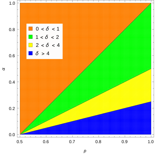
Refer to caption
Figure 1. A plot showing the regions for different types of behavior occurring for cookie environments as in Example 1.14.
Example 1.15 (Two-type, critical).

Let K=(1−ααα1−α)K=\begin{pmatrix}1-\alpha&\alpha\\ \alpha&1-\alpha\end{pmatrix} for some α∈(0,1)\alpha\in(0,1) and let 𝐩=(p,1−p)t\mathbf{p}=(p,1-p)^{t} for some p>1/2p>1/2. In this case, if we use the initial condition η=(1,0)\eta=(1,0) then a calculation done with Mathematica yields

(2) δ=δ⁡((1−ααα1−α),(p1−p),(1,0))=(2​p−1)​((2​α−1)​p−α)4​(2​α−1)​(p−1)​p+α−1.\delta=\delta\left(\begin{pmatrix}1-\alpha&\alpha\\ \alpha&1-\alpha\end{pmatrix},\begin{pmatrix}p\\ 1-p\end{pmatrix},(1,0)\right)=\frac{(2p-1)((2\alpha-1)p-\alpha)}{4(2\alpha-1)(p-1)p+\alpha-1}.

Note that if α∈(0,1/4)\alpha\in(0,1/4) then the parameter δ\delta is non-monotone in pp. In fact, for α<14−3​2156≈0.00450487\alpha<\frac{14-3\sqrt{21}}{56}\approx 0.00450487 the parameter δ\delta starts at 0, increases to a value larger than 44, and then decreases to 11 as pp ranges from 1/21/2 to 11 (See Figure 2).

Figure 2. The left plot shows the regions for different types of behavior occurring for cookie environments as in Example 1.15. The right plot shows the value of δ\delta as a function of p∈(1/2,1)p\in(1/2,1) when α=0.002\alpha=0.002.

Note also that the case α=0\alpha=0 corresponds to a classical simple random walk which steps to the right with probability p>1/2p>1/2 on each step. However, taking α=0\alpha=0 in (2) gives δ=p2​p−1\delta=\frac{p}{2p-1} and thus the results of Theorems 1.7 and 1.8 clearly do not hold when α=0\alpha=0 (this is not a contradiction since the transition matrix KK is the identity matrix when α=0\alpha=0 and there is more than one irreducible closed set). The case α=1\alpha=1 gives periodic cookie stacks with period 22 and the formula (2) gives δ=(2​p−1)​(1−p)4​p​(1−p)\delta=\frac{(2p-1)(1-p)}{4p(1-p)} which agrees with the formula obtained in [KOS14], see Example 1.13.

1.5. Structure of the paper

In Section 2 we introduce our main tool, forward and backward BLP, and show how the main results in the critical case (Theorems 1.6 - 1.8) can be deduced from Theorems 2.6 and 2.7 about the behavior of the tails of the lifetime and the total progeny over a lifetime of these BLP. Much of the remainder of the paper therefore is focused on the analysis of these BLPs, with the goal of proving Theorems 2.6 and 2.7. Section 3 discusses the asymptotics of the mean and variance of the forward BLP. Section 4 extends the results of the previous section to the backward BLP and establishes key relationships between parameters of the BLPs; in particular, in Section 4 we give explicit formulas for δ\delta and δ~\tilde{\delta}. In Section 5 we treat the non-critical case (p¯≠1/2\bar{p}\neq 1/2) deriving Theorem 1.5. Using the formulas for the parameters of the BLPs derived in the previous sections, we show how the BLPs in the non-critical case p¯>1/2\bar{p}>1/2 can be coupled with critical BLPs for which the parameter δ\delta is arbitrarily large. From this coupling we then show that the conclusions of Theorem 1.5 can be derived from Theorems 2.6 and 2.7 in the same way as the proofs of Theorems 1.6–1.8 were obtained when δ>4\delta>4. Finally, in Sections 6 and 7 we discuss proofs of Theorems  2.6 and 2.7. The crucial step here is showing that the BLPs have scaling limits that are squared Bessel processes. The generalized dimensions of these squared Bessel processes depend on the asymptotics of the mean and variance of the BLPs computed in Sections 3 and 4. This provides the connection of the parameters δ\delta and δ~\tilde{\delta} defined in Section 4 with the tail asymptotics exponents in Theorems 2.6 and 2.7.

2. The associated branching-like processes

In this section, we introduce two BLPs that are naturally associated with the ERW and will prove the main theorems for the critical case assuming the necessary results about these BLP.

Given a cookie environment ω\omega, we will expand the measure PωP_{\omega} to include an independent family of Bernoulli random variables {ξx​(j)}x∈ℤ,j≥1\{\xi_{x}(j)\}_{x\in\mathbb{Z},\,j\geq 1} such that ξx​(j)∼Bernoulli​(ωx​(j))\xi_{x}(j)\sim\text{Bernoulli}(\omega_{x}(j)). The ERW can then be constructed from the ξx​(j)\xi_{x}(j) as follows: if Xn=xX_{n}=x and ∑k=0n𝟏{Xk=x}=j\sum_{k=0}^{n}\mathbf{1}_{\{X_{k}=x\}}=j, then Xn+1=Xn+2​ξx​(j)−1X_{n+1}=X_{n}+2\xi_{x}(j)-1.

Remark 2.1.

The arrow systems construction of the ERW introduced by Holmes and Salisbury [HS12] is very similar to the above coin toss construction: compare the last equation with [Hol15, p. 2, above Theorem 1.1]. The distinction lies in the emphasis of the arrow approach on combinatorial results obtained by coupling of arrow systems rather than probability measures.

We now show how the family of Bernoulli random variables {ξx​(j)}\{\xi_{x}(j)\} can also be used to construct the associated forward and backward BLP.

2.1. The forward branching-like process

The excursions of a random walk to the right of the origin induce a natural tree-like structure on the right-directed edge local times of the walk. That is, for x≥1x\geq 1 jumps from xx to x+1x+1 can be thought of “descendants” of previous jumps from x−1x-1 to xx. To be precise, if we set γ0=0\gamma_{0}=0 and for n≥1n\geq 1 and x≥0x\geq 0 let

γn=inf{k>γn−1:Xk−1>0​ and ​Xk=0}andℰxn=∑k=0γn−1𝟏{Xk=x,Xk+1=x+1},\gamma_{n}=\inf\{k>\gamma_{n-1}:\,X_{k-1}>0\text{ and }X_{k}=0\}\quad\text{and}\quad\mathcal{E}_{x}^{n}=\sum_{k=0}^{\gamma_{n}-1}\mathbf{1}_{\{X_{k}=x,\,X_{k+1}=x+1\}},

then γn\gamma_{n} is the time of the nn-th return to the origin from the right and ℰxn\mathcal{E}_{x}^{n} is the number of times the random walk has traversed the directed edge from xx to x+1x+1 by time γn\gamma_{n} (note that γn\gamma_{n} can be infinite if the walk is transient to the right or left).

If the random walk makes nn excursions to the right (γn<∞\gamma_{n}<\infty), then the directed edge local times ℰxn\mathcal{E}_{x}^{n} can be computed from the Bernoulli random variables. If ℰx−1n=m\mathcal{E}_{x-1}^{n}=m, then since the steps of the random walk are ±1\pm 1 it follows that the walk makes mm jumps to the left from xx by time γn\gamma_{n}. Thus, ℰxn\mathcal{E}_{x}^{n} is the number of jumps that the random walk makes to the right from xx before the mm-th jump to the left. If we refer to a Bernoulli random variable ξx​(j)\xi_{x}(j) as a “success” if ξx​(j)=1\xi_{x}(j)=1 and a “failure” if ξx​(j)=0\xi_{x}(j)=0, then ℰxn\mathcal{E}_{x}^{n} is the number of successes in the Bernoulli sequence ξx={ξx​(j)}j≥1\xi_{x}=\{\xi_{x}(j)\}_{j\geq 1} before the mm-th failure. More precisely, introducing the notation

Smx=inf{k≥0:∑j=1k+m(1−ξx​(j))=m},S_{m}^{x}=\inf\left\{k\geq 0:\sum_{j=1}^{k+m}(1-\xi_{x}(j))=m\right\},

we have that if γn<∞\gamma_{n}<\infty and ℰx−1n=m\mathcal{E}_{x-1}^{n}=m then ℰxn=Smx\mathcal{E}_{x}^{n}=S_{m}^{x}. Note that S0x=0S_{0}^{x}=0 by the convention that an empty sum is equal to zero. Also, let Gmx=Smx−Sm−1xG_{m}^{x}=S_{m}^{x}-S_{m-1}^{x} so that GmxG_{m}^{x} is the number of successes between the (m−1)(m-1)-st failure and the mm-th failure in the Bernoulli sequence ξx\xi_{x}.

With the above directed edge process ℰxn\mathcal{E}_{x}^{n} as motivation, we define the forward BLP started at y≥1y\geq 1 by

(3) U0=yandUi=SUi−1i=∑m=1Ui−1Gmifor ​i≥1.U_{0}=y\quad\text{and}\quad U_{i}=S_{U_{i-1}}^{i}=\sum_{m=1}^{U_{i-1}}G_{m}^{i}\quad\text{for }i\geq 1.

We will use the notation PωU,y​(⋅)P_{\omega}^{U,y}(\cdot) and PηU,y​(⋅)=𝔼η​[PωU,y​(⋅)]P_{\eta}^{U,y}(\cdot)=\mathbb{E}_{\eta}[P_{\omega}^{U,y}(\cdot)] for the quenched and averaged distributions, respectively, of the forward BLP started at yy. Note that under the quenched measure PωU,yP_{\omega}^{U,y} the forward BLP is a time-inhomogeneous Markov chain, but since the cookie environment is assumed to be spatially i.i.d. the forward BLP is a time-homogeneous Markov chain under the averaged measure PηU,yP_{\eta}^{U,y} for any initial distribution η\eta.

The following Lemma summarizes the connection of the forward BLP with the directed edge local times of the random walk.

Lemma 2.2.

If U0=n≥1U_{0}=n\geq 1, then Ui≥ℰinU_{i}\geq\mathcal{E}_{i}^{n} for all i≥0i\geq 0. Moreover, on the event {γn<∞}\{\gamma_{n}<\infty\} we have Ui=ℰinU_{i}=\mathcal{E}_{i}^{n} for all i≥0i\geq 0 if U0=nU_{0}=n.

The equality Ui=ℰinU_{i}=\mathcal{E}_{i}^{n} on the event {γn<∞}\{\gamma_{n}<\infty\} was described above. For the proof of the general inequality Ui≥ℰinU_{i}\geq\mathcal{E}_{i}^{n} we refer the reader to [KZ08, Section 4] or [Pet13, Lemma 2.1].

Remark 2.3.

Note that in the case of classical simple random walks (i.e., ωx​(j)≡p∈(0,1)\omega_{x}(j)\equiv p\in(0,1)) {Gmi}i∈ℤ,m≥1\{G_{m}^{i}\}_{i\in\mathbb{Z},\,m\geq 1} is a sequence of i.i.d. Geometric(1−p1-p) random variables. In this case, it is clear from (3) that UiU_{i} is a branching process with Geometric(1−p1-p) offspring distribution. For ERWs with boundedly many cookies per site the GmiG_{m}^{i} are i.i.d. Geometric(1/21/2) for all mm sufficiently large and thus one can interpret UiU_{i} as a branching process with (random) migration (c.f. [KZ08], or more explicitly but in the context of the backward BLP see [BS08a]). However, in the more general setup of the current paper one can no longer interpret UiU_{i} as a branching process and so we simply refer to UiU_{i} as a “branching-like” process.

Remark 2.4.

One can also obtain a similar BLP which is related to the excursions of the ERW to the left of the origin. Clearly this BLP would have the same law as the forward BLP UiU_{i} defined here but with 𝐩\mathbf{p} replaced by 𝟏−𝐩\mathbf{1}-\mathbf{p}.

2.2. The backward branching-like process

The backward BLP is related to the random walk through edge local times. However, the backward BLP is related to the local times of the left directed edges when the random walk first reaches a fixed point to the right of the origin. To be precise,

𝒟nx=∑k=0Tn−1𝟏{Xk=x,Xk+1=x−1},n≥1,x<n,\mathcal{D}_{n}^{x}=\sum_{k=0}^{T_{n}-1}\mathbf{1}_{\{X_{k}=x,\,X_{k+1}=x-1\}},\quad n\geq 1,\,x<n,

be the number of steps to the left from xx before time TnT_{n} (recall that Tn=inf{k≥0:Xk=n}T_{n}=\inf\{k\geq 0:X_{k}=n\} is the hitting time of nn by the ERW). On the event {Tn<∞}\{T_{n}<\infty\}, the sequence of directed edge local times {𝒟nx}x≤n\{\mathcal{D}_{n}^{x}\}_{x\leq n} also have a branching-like structure. Jumps to the left from x+1x+1 before time TnT_{n} give rise to subsequent jumps to the left from xx before time TnT_{n}. However, one important difference with the forward BLP should be noted in that not all jumps to the left from xx are “descendants” of jumps to the left from x+1x+1. In particular, for x≥0x\geq 0 the random walk can jump to the left from xx before ever jumping from xx to x+1x+1.

As with ℰxn\mathcal{E}_{x}^{n} above, the directed edge process 𝒟nx\mathcal{D}_{n}^{x} can be computed from the Bernoulli random variables ξx​(j)\xi_{x}(j). In particular, if

Fmx=inf{k≥0:∑j=1k+mξx​(j)=m}F_{m}^{x}=\inf\left\{k\geq 0:\sum_{j=1}^{k+m}\xi_{x}(j)=m\right\}

denotes the number of failures in the Bernoulli sequence ξx={ξx​(j)}j≥1\xi_{x}=\{\xi_{x}(j)\}_{j\geq 1} before the mm-th success then it is easy to see that if Tn<∞T_{n}<\infty then 𝒟nn=0\mathcal{D}_{n}^{n}=0 and

(4) if ​𝒟nx+1=mthen𝒟nx={Fm+1xx≥0Fmxx<0,for ​x<n.\text{if }\mathcal{D}_{n}^{x+1}=m\quad\text{then}\quad\mathcal{D}_{n}^{x}=\begin{cases}F_{m+1}^{x}&x\geq 0\\ F_{m}^{x}&x<0,\end{cases}\quad\text{for }x<n.

Indeed, if x≥0x\geq 0 and there are mm jumps from x+1x+1 to xx before time TnT_{n} then there must be m+1m+1 jumps from xx to x+1x+1 (the initial jump from xx to x+1x+1 plus mm more jumps which can be paired with a prior jump from x+1x+1 to xx). Thus, from the construction of the random walk via the Bernoulli random variables ξx​(j)\xi_{x}(j) above, it follows that the number of jumps from xx to x−1x-1 before time TnT_{n} is the number of failures before the (m+1)(m+1)-th success in the Bernoulli sequence ξx\xi_{x}. The explanation of (4) when x<0x<0 is similar, with the exception that all jumps to the right from xx can be paired with a prior jump to the left from x+1x+1.

Again with the directed edge local time process as motivation, we define the backward BLP started at y≥0y\geq 0 by

(5) V0=yandVi=FVi−1+1ifor ​i≥1.V_{0}=y\quad\text{and}\quad V_{i}=F_{V_{i-1}+1}^{i}\quad\text{for }i\geq 1.

We will use PωV,yP_{\omega}^{V,y} and PηV,yP_{\eta}^{V,y} to denote the quenched and averaged laws of the backward branching process started at y≥0y\geq 0. As with the forward BLP, ViV_{i} is a time-inhomogeneous Markov chain under the quenched measure and a time-homogeneous Markov chain under the averaged measure.

Lemma 2.5.

If n≥1n\geq 1 and Pη​(Tn<∞)=1P_{\eta}(T_{n}<\infty)=1, then the sequence (𝒟nn,𝒟nn−1,…,𝒟n1,𝒟n0)(\mathcal{D}_{n}^{n},\mathcal{D}_{n}^{n-1},\ldots,\mathcal{D}_{n}^{1},\mathcal{D}_{n}^{0}) has the same distribution under PηP_{\eta} as the sequence (V0,V1,…,Vn−1,Vn)(V_{0},V_{1},\ldots,V_{n-1},V_{n}) under the measure PηV,0P_{\eta}^{V,0}.

Proof.

For n≥1n\geq 1 let {ξx(n)​(j)}x∈ℤ,j≥1\{\xi^{(n)}_{x}(j)\}_{x\in\mathbb{Z},\,j\geq 1} be the family of Bernoulli random variables given by ξx(n)​(j)=ξn−x​(j)\xi_{x}^{(n)}(j)=\xi_{n-x}(j) for x∈ℤx\in\mathbb{Z} and j≥1j\geq 1, and let Vi(n)V_{i}^{(n)} be the backward BLP started at V0(n)=0V_{0}^{(n)}=0 but defined using the Bernoulli family {ξx(n)​(j)}\{\xi_{x}^{(n)}(j)\} in place of {ξx​(j)}\{\xi_{x}(j)\}. Then, it is clear from (4) and (5) on the event {Tn<∞}\{T_{n}<\infty\} that 𝒟nn−i=Vi(n)\mathcal{D}_{n}^{n-i}=V_{i}^{(n)} for i=0,1,…,ni=0,1,\ldots,n. Finally, since the cookie environments are spatially i.i.d., it follows that {ξx(n)​(j)}x∈ℤ,j≥1\{\xi_{x}^{(n)}(j)\}_{x\in\mathbb{Z},\,j\geq 1} and {ξx​(j)}x∈ℤ,j≥1\{\xi_{x}(j)\}_{x\in\mathbb{Z},\,j\geq 1} have the same distribution under the averaged measure Pη=𝔼η​[Pω​(⋅)]P_{\eta}=\mathbb{E}_{\eta}[P_{\omega}(\cdot)]. ∎

2.3. Proofs of the main results in the critical case

Here and throughout the remainder of the paper, we will use the following notation for hitting times of stochastic processes. If {Zj}j≥0\{Z_{j}\}_{j\geq 0} is a stochastic process, then for any x∈ℝx\in\mathbb{R} let σxZ\sigma_{x}^{Z} and τxZ\tau_{x}^{Z} be the hitting times

σxZ:=inf{j>0:Zj≤x}andτxZ:=inf{j≥0:Zj≥x}.\sigma_{x}^{Z}:=\inf\{j>0:\,Z_{j}\leq x\}\ \ \text{and}\ \ \tau_{x}^{Z}:=\inf\{j\geq 0:\ Z_{j}\geq x\}.

Usually the stochastic process ZZ will be either the forward or backward BLP, though occasionally we will also use this notation for other processes.

The analysis of the forward and backward BLP is key to the proofs of all the main results in this paper. In particular, all of the results in the critical case p¯=1/2\bar{p}=1/2 (Theorems 1.6–1.8) will follow from the following two Theorems.

Theorem 2.6.

Let p¯=1/2\bar{p}=1/2 and let δ\delta be given by (38). If UU is the forward BLP defined in (3), then

  • •

    If δ>1\delta>1 then PηU,y​(σ0U=∞)>0P_{\eta}^{U,y}(\sigma_{0}^{U}=\infty)>0 for all y≥1y\geq 1.

  • •

    If δ≤1\delta\leq 1 then for any y≥1y\geq 1 there are positive constants =\Cr​f​l​(y,η)=\Cr{fl}(y,\eta) and =\Cr​f​p​(y,η)=\Cr{fp}(y,\eta) such that

    (6) limn→∞n1−δ​PηU,y​(σ0U>n)=\Cr​f​landlimn→∞n(1−δ)/2​PηU,y​(∑j=0σ0U−1Uj>n)=\Cr​f​p,\lim_{n\to\infty}n^{1-\delta}P_{\eta}^{U,y}(\sigma_{0}^{U}>n)=\Cr{fl}\ \ \text{and}\ \ \lim_{n\to\infty}n^{(1-\delta)/2}P_{\eta}^{U,y}\left(\sum_{j=0}^{\sigma_{0}^{U}-1}U_{j}>n\right)=\Cr{fp},

    where for δ=1\delta=1 we replace n0n^{0} with ln⁡n\ln n.

Theorem 2.7.

Let p¯=1/2\bar{p}=1/2 and let δ\delta be given by (38). If VV is the backward BLP defined in (5), then

  • •

    If δ<0\delta<0 then PηV,y​(σ0V=∞)>0P_{\eta}^{V,y}(\sigma_{0}^{V}=\infty)>0 for all y≥0y\geq 0.

  • •

    If δ≥0\delta\geq 0 then for any y≥0y\geq 0 there are positive constants =\Cr​b​l​(y,η)=\Cr{bl}(y,\eta) and =\Cr​b​p​(y,η)=\Cr{bp}(y,\eta) such that

    (7) limn→∞nδ​PηV,y​(σ0V>n)=\Cr​b​landlimn→∞nδ/2​PηV,y​(∑j=0σ0V−1Vj>n)=\Cr​b​p,\lim_{n\to\infty}n^{\delta}P_{\eta}^{V,y}(\sigma_{0}^{V}>n)=\Cr{bl}\ \ \text{and}\ \ \lim_{n\to\infty}n^{\delta/2}P_{\eta}^{V,y}\left(\sum_{j=0}^{\sigma_{0}^{V}-1}V_{j}>n\right)=\Cr{bp},

    where for δ=0\delta=0 we replace n0n^{0} with ln⁡n\ln n.

Remark 2.8.

Analogous theorems are known for the ERW with bounded number of cookies per site, [KM11, Theorems 2.1, 2.2], [DK15, Theorem 1.3].

We will give the proofs of Theorems 2.6 and 2.7 in Sections 6 and 7 below, but first we will show how they are used to prove Theorems 1.6–1.8.

Proof of Theorem 1.6.

For any cookie environment ω\omega, let ω+\omega^{+} be the modified cookie environment in which ωx+​(j)=ωx​(j)\omega^{+}_{x}(j)=\omega_{x}(j) for x≠0x\neq 0, j≥1j\geq 1 and with ω0+​(j)=1\omega^{+}_{0}(j)=1 for all j≥1j\geq 1 (that is, in the cookie environment ω+\omega^{+} the walk steps to the right after every visit to the origin). Recall that γn\gamma_{n} is the time of the nn-th return to the origin. Lemma 2.2 implies that

(8) Pω+​(γn<∞)=Pω+​(ℰnx=0, for all x sufficiently large)≤PωU,n​(σ0U<∞).P_{\omega^{+}}(\gamma_{n}<\infty)=P_{\omega^{+}}(\mathcal{E}_{n}^{x}=0,\text{ for all $x$ sufficiently large})\leq P_{\omega}^{U,n}(\sigma_{0}^{U}<\infty).

(Note that in the last probability on the right we can change the cookie environment from ω+\omega^{+} to ω\omega since the forward branching process is generated using the Bernoulli random variables ξx​(j)\xi_{x}(j) with x≥1x\geq 1.) If instead γn=∞\gamma_{n}=\infty, then since the ωx​(j)\omega_{x}(j) are uniformly bounded away from 00 and 11 the walk cannot stay bounded for the first nn excursions to the right. Therefore,

(9) Pω+(γn=∞)=Pω+(ℰnx≥1,∀x≥1)≤PωU,n(σ0U=∞),P_{\omega^{+}}(\gamma_{n}=\infty)=P_{\omega^{+}}(\mathcal{E}_{n}^{x}\geq 1,\,\forall x\geq 1)\leq P_{\omega}^{U,n}(\sigma_{0}^{U}=\infty),

where the last inequality follows from Lemma 2.2. Combining (8) and (9) we can conclude that

(10) Pω+​(γn<∞)=PωU,n​(σ0U<∞),∀n≥1.P_{\omega^{+}}(\gamma_{n}<\infty)=P_{\omega}^{U,n}(\sigma_{0}^{U}<\infty),\quad\forall n\geq 1.

Suppose that δ≤1\delta\leq 1. Then it follows from (10) and Theorem 2.6 that Eη​[Pω+​(γn<∞)]=1E_{\eta}[P_{\omega^{+}}(\gamma_{n}<\infty)]=1 for all n≥1n\geq 1. That is, with probability one every excursion of the ERW to the right of the origin will eventually return to the origin. Similarly, if δ~≤1\tilde{\delta}\leq 1 then all excursions to the left of the origin eventually return to the origin. Therefore, if δ,δ~≤1\delta,\tilde{\delta}\leq 1 then all excursions from the origin are finite and so the walk returns to the origin infinitely many times. Since all ωx​(j)\omega_{x}(j) are uniformly bounded away from 00 and 11 this implies that the walk visits every site infinitely often.

If instead δ>1\delta>1, then (10) and Theorem 2.6 imply that Eη​[Pω+​(γ1=∞)]>0E_{\eta}[P_{\omega^{+}}(\gamma_{1}=\infty)]>0, and thus

0<Eη​[ω0​(1)]​Eη​[Pω+​(γ1=∞)]\displaystyle 0<E_{\eta}[\omega_{0}(1)]E_{\eta}[P_{\omega^{+}}(\gamma_{1}=\infty)] ≤Pη​(Xn≥1,n≥1)≤Pη​(limn→∞Xn=∞),\displaystyle\leq P_{\eta}(X_{n}\geq 1,\,n\geq 1)\leq P_{\eta}\left(\lim_{n\rightarrow\infty}X_{n}=\infty\right),

where the last inequality again follows from the fact that the ωx​(j)\omega_{x}(j) are uniformly bounded away from 00 and 11. Finally, we can conclude by Theorem 1.4 that δ>1\delta>1 implies that the walk is transient to the right with probability 11. A similar argument shows that δ~>1\tilde{\delta}>1 implies that the walk is transient to the left. ∎

Proof of Theorem 1.7.

Since the limiting speed v0v_{0} exists by Theorem 1.4(ii), if the walk is recurrent then the speed must be v0=0v_{0}=0. Thus, we need only to consider the case where the walk is transient. First, assume that the walk is transient to the right (δ>1\delta>1). Since Tn/n=Tn/XTnT_{n}/n=T_{n}/X_{T_{n}}, the existence of the limiting speed v0v_{0} implies that limn→∞Tn/n=1/v0\lim_{n\rightarrow\infty}T_{n}/n=1/v_{0}, where we use the convention 1/0=∞1/0=\infty. It is easy to see that Tn=n+2​∑x<n𝒟nxT_{n}=n+2\sum_{x<n}\mathcal{D}_{n}^{x} for every n≥1n\geq 1. Since the walk is transient to the right,

(11) limn→∞2∑x<0𝒟nx≤∑k=0∞𝟏{Xk≤−1}<∞,\lim_{n\rightarrow\infty}2\sum_{x<0}\mathcal{D}_{n}^{x}\leq\sum_{k=0}^{\infty}\mathbf{1}_{\{X_{k}\leq-1\}}<\infty,

and thus

1v0=limn→∞Tnn=limn→∞1n​(n+2​∑x<n𝒟nx)=1+limn→∞2n​∑x=0n−1𝒟nx.\frac{1}{v_{0}}=\lim_{n\rightarrow\infty}\frac{T_{n}}{n}=\lim_{n\rightarrow\infty}\frac{1}{n}\left(n+2\sum_{x<n}\mathcal{D}_{n}^{x}\right)=1+\lim_{n\rightarrow\infty}\frac{2}{n}\sum_{x=0}^{n-1}\mathcal{D}_{n}^{x}.

It follows from Lemma 2.5 that n−1​∑x=0n−1𝒟nxn^{-1}\sum_{x=0}^{n-1}\mathcal{D}_{n}^{x} has the same distribution as n−1​∑i=1nVin^{-1}\sum_{i=1}^{n}V_{i} started with V0=0V_{0}=0, and standard Markov chain arguments imply that

limn→∞1n​∑i=1nVi=EηV,0​[∑i=0σ0V−1Vi]EηV,0​[σ0V],PηV,0​-a.s.\lim_{n\rightarrow\infty}\frac{1}{n}\sum_{i=1}^{n}V_{i}=\frac{E_{\eta}^{V,0}\left[\sum_{i=0}^{\sigma_{0}^{V}-1}V_{i}\right]}{E_{\eta}^{V,0}[\sigma_{0}^{V}]},\quad P_{\eta}^{V,0}\text{-a.s.}

Thus, we can conclude that

v0=(1+2​EηV,0​[∑i=0σ0V−1Vi]EηV,0​[σ0V])−1.v_{0}=\left(1+2\frac{E_{\eta}^{V,0}\left[\sum_{i=0}^{\sigma_{0}^{V}-1}V_{i}\right]}{E_{\eta}^{V,0}[\sigma_{0}^{V}]}\right)^{-1}.

Theorem 2.7 implies that the EηV,0​[σ0V]<∞E_{\eta}^{V,0}[\sigma_{0}^{V}]<\infty (recall that δ>1\delta>1 since the walk is transient to the right) and that EηV,0​[∑i=0σ0V−1Vi]<∞E_{\eta}^{V,0}[\sum_{i=0}^{\sigma_{0}^{V}-1}V_{i}]<\infty if and only if δ>2\delta>2. Thus we can conclude that v0>0⇔δ>2v_{0}>0\iff\delta>2. Again, a symmetric argument for random walks that are transient to the left shows that v0<0⇔δ~>2v_{0}<0\iff\tilde{\delta}>2. ∎

Proof of Theorem 1.8.

The proofs of the limiting distributions in Theorem 1.8 relies on the connection of the hitting times TnT_{n} with the backward BLP ViV_{i} from Lemma 2.5 and the tail asymptotics for the backward BLP in (7). We will give a brief sketch of the general argument here and will give full details in the case δ=2\delta=2 in Appendix B. We will refer the reader to previous papers for the details in all other cases.

For the limiting distributions of the hitting times TnT_{n}, recall that

(12) Tn=n+2​∑x=0n−1𝒟nx+2​∑x<0𝒟nx.T_{n}=n+2\sum_{x=0}^{n-1}\mathcal{D}_{n}^{x}+2\sum_{x<0}\mathcal{D}_{n}^{x}.

It follows from (11) that the third term on the right has a finite limit as n→∞n\rightarrow\infty, PηP_{\eta}-a.s., and therefore it is enough to prove a limiting distribution for the first two terms on the right side of (12). By Lemma 2.5 this is equivalent to proving a limiting distribution for n+2​∑i=1nVin+2\sum_{i=1}^{n}V_{i} under the measure PηV,0P_{\eta}^{V,0}. The proof of the limiting distribution for the partial sums of the BLP relies on the regeneration structure of the process ViV_{i}. Let rkr_{k} denote the time of the kk-th return of the backward BLP to zero. That is,

r0=0andrk=inf{i>rk−1:Vi=0}.r_{0}=0\quad\text{and}\quad r_{k}=\inf\{i>r_{k-1}:\,V_{i}=0\}.

Also, let Wk=∑i=rk−1rk−1ViW_{k}=\sum_{i=r_{k-1}}^{r_{k}-1}V_{i}. Note that {(rk−rk−1,Wk)}k≥1\{(r_{k}-r_{k-1},W_{k})\}_{k\geq 1} is an i.i.d. sequence under the measure PηV,0P_{\eta}^{V,0} and that Theorem 2.7 implies that r1r_{1} and W1W_{1} are in the domains of attraction of totally asymmetric stable distributions of index min⁡{δ,2}\min\{\delta,2\} and min⁡{δ/2,2}\min\{\delta/2,2\}, respectively. From this, the limiting distributions for n+2​∑i=1nVin+2\sum_{i=1}^{n}V_{i} are standard. For the details of the arguments in cases (i)-(v) we give the following references.

  • •

    δ∈(1,2)\delta\in(1,2): See [BS08b], pages 847–849.

  • •

    δ=2\delta=2: See Appendix B.

  • •

    δ∈(2,4]\delta\in(2,4]: See Section 9 in [KM11].

  • •

    δ>4\delta>4: By (7) the second moment of the random variable ∑j=0σ0V−1Vj\sum_{j=0}^{\sigma_{0}^{V}-1}V_{j} is finite. Thus, this is a classical case covered by the standard CLT for the Markov chain VV; see, for example, [Chu67, I.16, Theorem 1].55 5 For the second statement of (v) see also [KZ08], proof of Theorem 3 and Section 6. The argument is based on the result due to A.-S. Sznitman [Szn00, Theorem 4.1] and gives the functional CLT for the position of the walk.

Finally, to obtain the limiting distributions for the position XnX_{n} of the ERW from the limiting distributions of the hitting times TnT_{n}, we use the fact that

(13) {Tm>n}⊂{Xn<m}⊂{Tm+r>n}∪{infk≥Tm+rXk<m},\{T_{m}>n\}\subset\{X_{n}<m\}\subset\{T_{m+r}>n\}\cup\left\{\inf_{k\geq T_{m+r}}X_{k}<m\right\},

for any m,n,r≥1m,n,r\geq 1. The key then is to control the probability of the last event on the right. To this end, it was shown in [Pet12, Lemma 6.1] that the tail asymptotics for r1r_{1} in (7) imply that

(14) Pη​(infk≥Tm+rXk<m)≤C​r1−δ,∀m,r≥1.P_{\eta}\left(\inf_{k\geq T_{m+r}}X_{k}<m\right)\leq Cr^{1-\delta},\quad\forall m,r\geq 1.

Again, for the details of how to use (13) and (14) to obtain the limiting distributions for XnX_{n}, see the references given above. ∎

3. Mean and variance of the forward BLP

Many of the calculations below are simplified using matrix notation.

  • •

    𝟏\mathbf{1} will denote a column vector of all ones, and 𝐩\mathbf{p} denotes a column vector with ii-th entry p⁡(i)p(i).

  • •

    II is the identity matrix.

  • •

    DpD_{p} will denote a diagonal matrix with ii-th diagonal entry p⁡(i)p(i). Similarly D1−p=I−DpD_{1-p}=I-D_{p} is the diagonal matrix with ii-th diagonal entry 1−p⁡(i)1-p(i).

  • •

    Recall that p¯=μ⋅𝐩\bar{p}=\mu\cdot\mathbf{p}, where μ\mu is the stationary distribution for the environment Markov chain.

In this section and the next section, we will be concerned with a single increment of the BLP. Thus, we will only need to consider the environment at any fixed site x∈ℤx\in\mathbb{Z}. Therefore, in this section we will fix xx and suppress the sub/super-script xx for a less cumbersome notation. For instance, we will write Rj=RjxR_{j}=R_{j}^{x} for the Markov chain which generates the environment at xx and the Bernoulli sequence is denoted {ξ⁡(j)}j≥1={ξx​(j)}j≥1\{\xi(j)\}_{j\geq 1}=\{\xi_{x}(j)\}_{j\geq 1}.

3.1. Mean

Proposition 3.1.

For every distribution η\eta on ℛ{\cal R}

limn→∞EηU,n​[U1]n=p¯1−p¯=:λ.\lim_{n\rightarrow\infty}\frac{E_{\eta}^{U,n}[U_{1}]}{n}=\frac{\bar{p}}{1-\bar{p}}=:\lambda.

Moreover, there exist constants ,>0,>0 such that for any n∈ℕn\in\mathbb{N} and any distribution η\eta on ℛ\mathcal{R}

(15) |EηU,n​[U1]−λ​n−η⋅𝐫|≤\Cr​m​l​e−\Cr​m​u​n,\left|E_{\eta}^{U,n}[U_{1}]-\lambda n-\eta\cdot\mathbf{r}\right|\leq\Cr{ml}e^{-\Cr{mu}n},

where

(16) 𝐫=𝐫⁡(𝐩,K)=(I−K+(𝟏−𝐩)​μ​D1−p​K1−p¯)−1​𝐩−λ​𝟏.\mathbf{r}=\mathbf{r}(\mathbf{p},K)=\left(I-K+\frac{(\mathbf{1-p})\mu D_{1-p}K}{1-\bar{p}}\right)^{-1}\mathbf{p}-\lambda\mathbf{1}.
Proof.

Recall that SmS_{m} is the number of successes before the mm-th failure in the Bernoulli sequence ξ={ξ⁡(j)}j≥1\xi=\{\xi(j)\}_{j\geq 1}, and let Gm=Sm−Sm−1G_{m}=S_{m}-S_{m-1} be the number of successes between the (m−1)(m-1)-st and the mm-th failure in the Bernoulli sequence ξ\xi. With this notation it follows from the construction of the forward BLP in Section 2 that

(17) EηU,n​[U1]=∑m=1nEη​[Gm].E_{\eta}^{U,n}[U_{1}]=\sum_{m=1}^{n}E_{\eta}[G_{m}].

To compute Eη​[Gm]E_{\eta}[G_{m}] it helps to keep track of some additional information. Let I0=R1I_{0}=R_{1} and for any m≥1m\geq 1 let ImI_{m} be defined by

Im=RSm+m+1.I_{m}=R_{S_{m}+m+1}.

Note that Sm+mS_{m}+m is the number of Bernoulli trials needed to obtain mm failures. Therefore, Im=iI_{m}=i if the next Bernoulli random variable after the mm-th failure has success probability p⁡(i)p(i). Since

Pη({ξ(j)}j≥Sm+m+1∈⋅|σ(ξ(j),j≤Sm+m+1))=PIm({ξ(j)}j≥1∈⋅),P_{\eta}(\{\xi(j)\}_{j\geq S_{m}+m+1}\in\cdot\,|\,\sigma(\xi(j),\,j\leq S_{m}+m+1))=P_{I_{m}}(\{\xi(j)\}_{j\geq 1}\in\cdot),

it follows that {Im}m≥0\{I_{m}\}_{m\geq 0} is a Markov chain on the state space ℛ\mathcal{R}. By the ellipticity assumption, p:ℛ→(0,1)p:{\cal R}\to(0,1), the Markov chain {Im}m≥0\{I_{m}\}_{m\geq 0} has the same unique closed irreducible subset ℛ0\mathcal{R}_{0} as the Markov chain {Rj}j≥1\{R_{j}\}_{j\geq 1}. Therefore, {Im}m≥0\{I_{m}\}_{m\geq 0} has a unique stationary distribution π\pi. While we did not assume any aperiodicity for {Rj}j≥0\{R_{j}\}_{j\geq 0}, the ellipticity assumption implies that {Im}m≥0\{I_{m}\}_{m\geq 0} is aperiodic, and since ℛ{\cal R} is finite the convergence to stationarity is exponentially fast: if Π\Pi is the matrix of transition probabilities for the Markov chain ImI_{m}, then there exist constants ,>0,>0 such that

(18) supη‖η​Πn−π‖∞≤\Cr​s​l​e−\Cr​s​u​n,∀n≥1,\sup_{\eta}\|\eta\Pi^{n}-\pi\|_{\infty}\leq\Cr{sl}e^{-\Cr{su}n},\quad\forall n\geq 1,

where the supremum on the left is over all probability measures η\eta on ℛ\mathcal{R}.

Let 𝐠\mathbf{g} denote the column vector of length NN with ii-th entry g⁡(i)=Ei​[G1]g(i)=E_{i}[G_{1}]. Note that by the comparison with a geometric random variable with parameter pmax:=maxi∈ℛ⁡p⁡(i)<1p_{\text{max}}:=\max_{i\in{\cal R}}p(i)<1 we see that g⁡(i)<pmax/(1−pmax)<∞g(i)<p_{\text{max}}/(1-p_{\text{max}})<\infty for every i∈ℛi\in\mathcal{R}. Then, since Eη​[Gm]=Eη​[g⁡(Im−1)]E_{\eta}[G_{m}]=E_{\eta}[g(I_{m-1})] it follows from an ergodic theorem for finite state Markov chains that

limn→∞1n​EηU,n​[U1]=limn→∞1n​∑m=1nEη​[Gm]=Eπ​[g⁡(I0)]=∑i∈ℛπ⁡(i)​g​(i)=π⋅𝐠.\lim_{n\rightarrow\infty}\frac{1}{n}E_{\eta}^{U,n}[U_{1}]=\lim_{n\rightarrow\infty}\frac{1}{n}\sum_{m=1}^{n}E_{\eta}[G_{m}]=E_{\pi}[g(I_{0})]=\sum_{i\in\mathcal{R}}\pi(i)g(i)=\pi\cdot\mathbf{g}.

Therefore, to prove the first part of the lemma we need to show that π⋅𝐠=λ\pi\cdot\mathbf{g}=\lambda. The following lemma accomplishes this task. It also provides useful information about {Im}m≥0\{I_{m}\}_{m\geq 0} which we need in the rest of this section.

Lemma 3.2.

The sequence {Im}m≥0\{I_{m}\}_{m\geq 0} is a Markov chain with transition probabilities given by the matrix

Π=(I−Dp​K)−1​D1−p​K,\Pi=(I-D_{p}K)^{-1}D_{1-p}K,

and with a unique stationary distribution π\pi given by

(19) π=μ⁡(I−Dp​K)1−p¯=(1+λ)​μ​(I−Dp​K).\pi=\frac{\mu(I-D_{p}K)}{1-\bar{p}}=(1+\lambda)\mu(I-D_{p}K).

Moreover,

(20) 𝐠=(I−Dp​K)−1​𝐩andπ⋅𝐠=λ.\mathbf{g}=(I-D_{p}K)^{-1}\mathbf{p}\quad\text{and}\quad\pi\cdot\mathbf{g}=\lambda.
Remark 3.3.

In the first formula for π\pi in (19), the multiplicative factor 1/(1−p¯)1/(1-\bar{p}) is needed for the entries of π\pi to sum to 1 since μ⁡(I−Dp​K)​𝟏=μ⁡(𝟏−𝐩)=1−p¯\mu(I-D_{p}K)\mathbf{1}=\mu(\mathbf{1}-\mathbf{p})=1-\bar{p}. The second formula for π\pi in (19) is equivalent since λ=p¯1−p¯\lambda=\frac{\bar{p}}{1-\bar{p}} implies that 11−p¯=1+λ\frac{1}{1-\bar{p}}=1+\lambda.

Proof.

To compute the transition probabilities, for k≥0k\geq 0 let MkM_{k} be the N×NN\times N matrix with entries

Mk​(i,i′)=Pi​(G1=k,I1=i′).M_{k}(i,i^{\prime})=P_{i}(G_{1}=k,I_{1}=i^{\prime}).

Obviously, M0​(i,i′)=(1−pi)​Ki,i′=(D1−p​K)i,i′M_{0}(i,i^{\prime})=(1-p_{i})K_{i,i^{\prime}}=(D_{1-p}K)_{i,i^{\prime}} and for k≥1k\geq 1 by conditioning on the value of R2R_{2} we obtain that

Mk​(i,i′)=∑ℓ=1Npi​Ki,ℓ​Mk−1​(ℓ,i′).M_{k}(i,i^{\prime})=\sum_{\ell=1}^{N}p_{i}K_{i,\ell}M_{k-1}(\ell,i^{\prime}).

That is, M0=D1−p​KM_{0}=D_{1-p}K and Mk=Dp​K​Mk−1M_{k}=D_{p}KM_{k-1} for k≥1k\geq 1. Combining these we get that Mk=(Dp​K)k​D1−p​KM_{k}=(D_{p}K)^{k}D_{1-p}K. Since Π⁡(i,i′)=∑k≥0Mk​(i,i′)\Pi(i,i^{\prime})=\sum_{k\geq 0}M_{k}(i,i^{\prime}), we have that

Π=∑k=0∞Mk=∑k=0∞(Dp​K)k​D1−p​K=(I−Dp​K)−1​D1−p​K.\Pi=\sum_{k=0}^{\infty}M_{k}=\sum_{k=0}^{\infty}(D_{p}K)^{k}D_{1-p}K=(I-D_{p}K)^{-1}D_{1-p}K.

(Note that since Dp​KD_{p}K is a matrix with non-negative entries and with ii-th row sum equal to p⁡(i)<1p(i)<1, the Perron-Frobenius theorem implies that all eigenvalues of Dp​KD_{p}K have absolute value strictly less than one, and thus I−Dp​KI-D_{p}K is invertible.) It it is easy to check that π​Π=π\pi\Pi=\pi by noting that μ​K=μ\mu K=\mu and, thus,

(21) μ​D1−p​K=μ⁡(I−Dp)​K=μ⁡(I−Dp​K).\mu D_{1-p}K=\mu(I-D_{p})K=\mu(I-D_{p}K).

Finally, we give a formula for 𝐠\mathbf{g}. For k≥1k\geq 1 one easily sees that

Pi​(G1≥k)=∑i1∈ℛp⁡(i)​Ki,i1​Pi1​(G1≥k−1).P_{i}(G_{1}\geq k)=\sum_{i_{1}\in\mathcal{R}}p(i)K_{i,i_{1}}P_{i_{1}}(G_{1}\geq k-1).

Iterating this, we obtain

(22) Pi(G1≥k)=∑i1,i2,…,ik∈ℛ(p(i)Ki,i1)(p(i1)Ki1,i2)⋯(p(ik−1)Kik−1,ik)=ei(DpK)k𝟏,P_{i}(G_{1}\geq k)=\sum_{i_{1},i_{2},\ldots,i_{k}\in\mathcal{R}}(p(i)K_{i,i_{1}})(p(i_{1})K_{i_{1},i_{2}})\cdots(p(i_{k-1})K_{i_{k-1},i_{k}})=e_{i}(D_{p}K)^{k}\mathbf{1},

where in the last equality we use the notation eie_{i} for the row vector with a one in the ii-th coordinate and zeros elsewhere. Therefore,

g⁡(i)=Ei​[G1]=∑k≥1Pi​(G1≥k)=∑k≥1ei​(Dp​K)k​𝟏=ei​(I−Dp​K)−1​Dp​K​𝟏=ei​(I−Dp​K)−1​𝐩g(i)=E_{i}[G_{1}]=\sum_{k\geq 1}P_{i}(G_{1}\geq k)=\sum_{k\geq 1}e_{i}(D_{p}K)^{k}\mathbf{1}=e_{i}(I-D_{p}K)^{-1}D_{p}K\mathbf{1}=e_{i}(I-D_{p}K)^{-1}\mathbf{p}

and we get (20) as claimed. From this and the formula for π\pi in (19) it follows immediately that π⋅𝐠=λ\pi\cdot\mathbf{g}=\lambda. ∎

In the critical case p¯=1/2\bar{p}=1/2, Lemma 3.2 and (21) give the following simpler formula for the stationary distribution π\pi that will be useful below.

Corollary 3.4.

If p¯=1/2\bar{p}=1/2 then π=2​μ​(I−Dp​K)=2​μ​D1−p​K\pi=2\mu(I-D_{p}K)=2\mu D_{1-p}K.

Thus far we have proved the first part of Proposition 3.1. Next we show the existence of a vector 𝐫\mathbf{r} such that (15) holds. To this end, for any n≥1n\geq 1 let 𝐫n=(rn​(1),rn​(2),…,rn​(N))t\mathbf{r}_{n}=(r_{n}(1),r_{n}(2),\ldots,r_{n}(N))^{t} be the column vector with ii-th entry

rn​(i)=EiU,n​[U1]−λ​n=∑m=1n(Ei​[Gm]−λ).r_{n}(i)=E_{i}^{U,n}[U_{1}]-\lambda n=\sum_{m=1}^{n}\left(E_{i}[G_{m}]-\lambda\right).

Then

𝐫n=∑m=1n(Πm−1​𝐠−𝟏​π⋅𝐠)=∑m=0n−1(Πm−𝟏​π)​𝐠,\mathbf{r}_{n}=\sum_{m=1}^{n}\left(\Pi^{m-1}\mathbf{g}-\mathbf{1}\pi\cdot\mathbf{g}\right)=\sum_{m=0}^{n-1}\left(\Pi^{m}-\mathbf{1}\pi\right)\mathbf{g},

where in the last equality the matrix 𝟏​π\mathbf{1}\pi is the N×NN\times N matrix with all rows equal to the vector π\pi which is the stationary distribution for {Im}m≥0\{I_{m}\}_{m\geq 0}. It follows from (18) that the entries of Πm−𝟏​π\Pi^{m}-\mathbf{1}\pi decrease exponentially in mm, so that the sum in the last line converges as n→∞n\rightarrow\infty. That is,

(23) limn→∞𝐫n=𝐫:=∑m=0∞(Πm−𝟏​π)​𝐠.\lim_{n\rightarrow\infty}\mathbf{r}_{n}=\mathbf{r}:=\sum_{m=0}^{\infty}\left(\Pi^{m}-\mathbf{1}\pi\right)\mathbf{g}.

Moreover, since EηU,n​[U1]−λ​n=η⋅𝐫nE_{\eta}^{U,n}[U_{1}]-\lambda n=\eta\cdot\mathbf{r}_{n}, then

|EηU,n​[U1]−λ​n−η⋅𝐫|=|η⋅(𝐫n−𝐫)|≤∑m=n∞‖η​Πm−π‖∞​‖𝐠‖1≤‖𝐠‖1​\Cr​s​l1−e−\Cr​s​u​e−\Cr​s​u​n,\left|E_{\eta}^{U,n}[U_{1}]-\lambda n-\eta\cdot\mathbf{r}\right|=\left|\eta\cdot\left(\mathbf{r}_{n}-\mathbf{r}\right)\right|\leq\sum_{m=n}^{\infty}\left\|\eta\Pi^{m}-\pi\right\|_{\infty}\|\mathbf{g}\|_{1}\leq\frac{\|\mathbf{g}\|_{1}\Cr{sl}}{1-e^{-\Cr{su}}}e^{-\Cr{su}n},

where the last inequality follows from (18).

Finally, we give an explicit formula for the vector 𝐫\mathbf{r}. To this end, since π​Π=π\pi\Pi=\pi it follows that (𝟏​π)​Π=𝟏​π=Π⁡(𝟏​π)(\mathbf{1}\pi)\Pi=\mathbf{1}\pi=\Pi(\mathbf{1}\pi) and thus (Πm−𝟏​π)=(Π−𝟏​π)m(\Pi^{m}-\mathbf{1}\pi)=(\Pi-\mathbf{1}\pi)^{m} for all m≥1m\geq 1. Therefore,

(24) 𝐫=(I−𝟏​π)​𝐠+∑m=1∞(Π−𝟏​π)m​𝐠=∑m=0∞(Π−𝟏​π)m​𝐠−(π⋅𝐠)​𝟏=(I−Π+𝟏​π)−1​𝐠−λ​𝟏.\mathbf{r}=(I-\mathbf{1}\pi)\mathbf{g}+\sum_{m=1}^{\infty}\left(\Pi-\mathbf{1}\pi\right)^{m}\mathbf{g}=\sum_{m=0}^{\infty}\left(\Pi-\mathbf{1}\pi\right)^{m}\mathbf{g}-(\pi\cdot\mathbf{g})\mathbf{1}=(I-\Pi+\mathbf{1}\pi)^{-1}\mathbf{g}-\lambda\mathbf{1}.

Substituting the expressions for π,Π\pi,\ \Pi, and 𝐠\mathbf{g} and simplifying we obtain (16). ∎

In closing this subsection, we note the following Corollary which will be of use later.

Corollary 3.5.

π⋅𝐫=0\pi\cdot\mathbf{r}=0.

Proof.

Since π\pi is the stationary distribution for the Markov chain with transition matrix Π\Pi it follows that π⁡(I−Π+𝟏​π)=π\pi(I-\Pi+\mathbf{1}\pi)=\pi, or equivalently π​(I−Π+𝟏​π)−1=π\pi(I-\Pi+\mathbf{1}\pi)^{-1}=\pi. Using the formula for 𝐫\mathbf{r} in (24), it follows that π⋅𝐫=π​(I−Π+𝟏​π)−1​𝐠−λ​π⋅𝟏=π⋅𝐠−λ=0\pi\cdot\mathbf{r}=\pi(I-\Pi+\mathbf{1}\pi)^{-1}\mathbf{g}-\lambda\pi\cdot\mathbf{1}=\pi\cdot\mathbf{g}-\lambda=0, where the last equality follows from (20).

∎

3.2. Variance

The main result of this subsection is the following proposition.

Proposition 3.6.

There exists a constant >0>0 such that for any distribution η\eta on ℛ{\cal R}

|Varη⁡(U1|U0=n)n−ν|≤\Cr​vn,\left|\frac{\Var_{\eta}(U_{1}|\,U_{0}=n)}{n}-\nu\right|\leq\frac{\Cr{v}}{n},

where the constant ν\nu is given by the formula

(25) ν=ν⁡(𝐩,K)=Varπ⁡(G1)+2​∑k=1∞Covπ⁡(G1,G1+k)=(1+λ)​(λ+2​μ​Dp​K​𝐫),\nu=\nu(\mathbf{p},K)=\Var_{\pi}(G_{1})+2\sum_{k=1}^{\infty}\Cov_{\pi}(G_{1},G_{1+k})=(1+\lambda)(\lambda+2\mu D_{p}K\mathbf{r}),

and 𝐫\mathbf{r} is the vector from Proposition 3.1. In particular, if p¯=1/2\bar{p}=1/2 then

(26) ν=2+4​μ​Dp​K​𝐫=4​μ​Dp​K​(I−K+2​(𝟏−𝐩)​μ​D1−p​K)−1​𝐩.\nu=2+4\mu D_{p}K\mathbf{r}=4\mu D_{p}K(I-K+2\mathbf{(1-p)}\mu D_{1-p}K)^{-1}\mathbf{p}.
Proof.

First note that for any measure η\eta on ℛ{\cal R},

Varη⁡(U1|U0=n)=Varη⁡(∑k=1nGk)\displaystyle\Var_{\eta}(U_{1}|\,U_{0}=n)=\Var_{\eta}\left(\sum_{k=1}^{n}G_{k}\right) =∑k=1nVarη⁡(Gk)+2​∑1≤k<ℓ≤nCovη⁡(Gk,Gℓ).\displaystyle=\sum_{k=1}^{n}\Var_{\eta}\left(G_{k}\right)+2\sum_{1\leq k<\ell\leq n}\Cov_{\eta}(G_{k},G_{\ell}).

Let νn=Varπ⁡(U1|U0=n)=Varπ⁡(∑k=1nGk)\nu_{n}=\Var_{\pi}(U_{1}|\,U_{0}=n)=\Var_{\pi}\left(\sum_{k=1}^{n}G_{k}\right). The proof will consist of three steps.

  • Step 1.

    Show that |νn−Varη⁡(U1|U0=n)|\left|\nu_{n}-\Var_{\eta}(U_{1}|\,U_{0}=n)\right| is bounded by a constant uniformly in nn and η\eta.

  • Step 2.

    Prove that there is a constant C>0C>0 such that |νn/n−ν|≤C/n\left|\nu_{n}/n-\nu\right|\leq C/n.

  • Step 3.

    Calculate ν\nu explicitly and show that (25) and (26) hold.

Step 1. For any k≥0k\geq 0 and i∈ℛi\in{\cal R} let vk​(i)=Ei​[G1​G1+k]v_{k}(i)=E_{i}[G_{1}G_{1+k}] and

𝐯k=(vk​(1),vk​(2),…,vk​(N))t.\mathbf{v}_{k}=(v_{k}(1),v_{k}(2),\ldots,v_{k}(N))^{t}.

With this notation, we have that

(27) Varη⁡(Gk)=η​Πk−1​𝐯0−(η​Πk−1​𝐠)2,∀k≥1,\Var_{\eta}(G_{k})=\eta\Pi^{k-1}\mathbf{v}_{0}-(\eta\Pi^{k-1}\mathbf{g})^{2},\quad\forall k\geq 1,

and

(28) Covη⁡(Gk,Gℓ)=η​Πk−1​𝐯ℓ−k−(η​Πk−1​𝐠)​(η​Πℓ−1​𝐠),∀1≤k<ℓ.\Cov_{\eta}(G_{k},G_{\ell})=\eta\Pi^{k-1}\mathbf{v}_{\ell-k}-(\eta\Pi^{k-1}\mathbf{g})(\eta\Pi^{\ell-1}\mathbf{g}),\quad\forall 1\leq k<\ell.

Note that in the special case where η\eta has distribution π\pi these become

(29) Varπ⁡(Gk)=π⁡(𝐯0−λ​𝐠),andCovπ⁡(Gk,Gℓ)=π⁡(𝐯ℓ−k−λ​𝐠),for ​1≤k<ℓ,\Var_{\pi}(G_{k})=\pi(\mathbf{v}_{0}-\lambda\mathbf{g}),\quad\text{and}\quad\Cov_{\pi}(G_{k},G_{\ell})=\pi(\mathbf{v}_{\ell-k}-\lambda\mathbf{g}),\quad\text{for }1\leq k<\ell,

since π​Π=π\pi\Pi=\pi and π⋅𝐠=λ\pi\cdot\mathbf{g}=\lambda. The following lemma is elementary.

Lemma 3.7.

supk≥0‖𝐯k‖∞<∞\sup_{k\geq 0}\|\mathbf{v}_{k}\|_{\infty}<\infty.

Proof.

First of all, note that the Cauchy-Schwartz inequality implies that

Ei​[G1​G1+k]≤Ei​[G12]​Ei​[G1+k2]≤maxi⁡Ei​[G12]=‖𝐯0‖∞,E_{i}[G_{1}G_{1+k}]\leq\sqrt{E_{i}[G_{1}^{2}]E_{i}[G_{1+k}^{2}]}\leq\max_{i}E_{i}[G_{1}^{2}]=\|\mathbf{v}_{0}\|_{\infty},

and thus it is enough to prove that Ei​[G12]<∞E_{i}[G_{1}^{2}]<\infty for every i∈ℛi\in\mathcal{R}. The last inequality is obvious by comparison with a geometric random variable with parameter pmax=maxi∈ℛ⁡p⁡(i)<1p_{\text{max}}=\max_{i\in{\cal R}}p(i)<1. ∎

Lemma 3.8.

There exist constants, ,>0,>0 so that for any distribution η\eta on ℛ{\cal R} and any 1≤k<ℓ1\leq k<\ell

(30) |Varη⁡(Gk)−Varπ⁡(Gk)|≤\Cr​v​l​e−\Cr​v​u​kand|Covη⁡(Gk,Gℓ)−Covπ⁡(Gk,Gℓ)|≤\Cr​v​l​e−\Cr​v​u​ℓ.\left|\Var_{\eta}(G_{k})-\Var_{\pi}(G_{k})\right|\leq\Cr{vl}e^{-\Cr{vu}k}\quad\text{and}\quad\left|\Cov_{\eta}(G_{k},G_{\ell})-\Cov_{\pi}(G_{k},G_{\ell})\right|\leq\Cr{vl}e^{-\Cr{vu}\ell}.
Proof.

The key observation is the exponential convergence to the stationary distribution π\pi for the Markov chain {Im}m≥0\{I_{m}\}_{m\geq 0} as noted in (18) above. From this, it follows easily that

|η​Πk−1​𝐯0−π⋅𝐯0|≤\Cr​s​l​‖𝐯0‖1​e−\Cr​s​u​(k−1)and|η​Πk−1​𝐠−π⋅𝐠|≤\Cr​s​l​‖𝐠‖1​e−\Cr​s​u​(k−1).|\eta\Pi^{k-1}\mathbf{v}_{0}-\pi\cdot\mathbf{v}_{0}|\leq\Cr{sl}\|\mathbf{v}_{0}\|_{1}e^{-\Cr{su}(k-1)}\quad\text{and}\quad|\eta\Pi^{k-1}\mathbf{g}-\pi\cdot\mathbf{g}|\leq\Cr{sl}\|\mathbf{g}\|_{1}e^{-\Cr{su}(k-1)}.

The first inequality in (30) then follows easily from the above bounds and the representations for the variances in (27) and (29) taking into account the fact that η​Πk−1\eta\Pi^{k-1} is always a probability distribution so that |η​Πk−1​𝐠+π⋅𝐠|≤2​‖𝐠‖∞|\eta\Pi^{k-1}\mathbf{g}+\pi\cdot\mathbf{g}|\leq 2\|\mathbf{g}\|_{\infty}.

To obtain the bound on the difference of the covariance terms in (30), note that the representations in (28) and (29) imply that

|Covη⁡(Gk,Gℓ)−Covπ⁡(Gk,Gℓ)|\displaystyle\left|\Cov_{\eta}(G_{k},G_{\ell})-\Cov_{\pi}(G_{k},G_{\ell})\right| ≤|η​Πk−1​𝐯ℓ−k−(η​Πk−1​𝐠)​(η​Πℓ−1​𝐠)−π⁡(𝐯ℓ−k−λ​𝐠)|\displaystyle\leq\left|\eta\Pi^{k-1}\mathbf{v}_{\ell-k}-(\eta\Pi^{k-1}\mathbf{g})(\eta\Pi^{\ell-1}\mathbf{g})-\pi(\mathbf{v}_{\ell-k}-\lambda\mathbf{g})\right|
≤|(η​Πk−1−π)​(𝐯ℓ−k−λ​𝐠)|+|η​Πk−1​𝐠|​|λ−η​Πℓ−1​𝐠|\displaystyle\leq\left|(\eta\Pi^{k-1}-\pi)(\mathbf{v}_{\ell-k}-\lambda\mathbf{g})\right|+\left|\eta\Pi^{k-1}\mathbf{g}\right|\left|\lambda-\eta\Pi^{\ell-1}\mathbf{g}\right|
≤\Cr​s​l​e−\Cr​s​u​(k−1)​‖𝐯ℓ−k−λ​𝐠‖1+‖𝐠‖∞​‖𝐠‖1​\Cr​s​l​e−\Cr​s​u​(ℓ−1),\displaystyle\leq\Cr{sl}e^{-\Cr{su}(k-1)}\|\mathbf{v}_{\ell-k}-\lambda\mathbf{g}\|_{1}+\|\mathbf{g}\|_{\infty}\|\mathbf{g}\|_{1}\Cr{sl}e^{-\Cr{su}(\ell-1)},

where the last inequality again follows from (18) and the fact that π⋅𝐠=λ\pi\cdot\mathbf{g}=\lambda. Therefore, it will be enough to show that there exist constants C,C′>0C,C^{\prime}>0 such that

(31) ‖𝐯k−λ​𝐠‖1≤C​‖𝐠‖12​e−C′​k,∀k≥1.\|\mathbf{v}_{k}-\lambda\mathbf{g}\|_{1}\leq C\|\mathbf{g}\|_{1}^{2}e^{-C^{\prime}k},\quad\forall k\geq 1.

To this end, note that by conditioning on (G1,I1)(G_{1},I_{1}) we get that

Ei​[G1​Gk+1]−λ​Ei​[G1]=∑i′∈ℛ∑n=0∞n​Pi​(G1=n,I1=i′)​(Ei′​[Gk]−λ).E_{i}[G_{1}G_{k+1}]-\lambda E_{i}[G_{1}]=\sum_{i^{\prime}\in\mathcal{R}}\sum_{n=0}^{\infty}nP_{i}(G_{1}=n,\,I_{1}=i^{\prime})\left(E_{i^{\prime}}[G_{k}]-\lambda\right).

By (18) maxi∈ℛ⁡|Ei​[Gk]−λ|=maxi∈ℛ⁡|ei​Πk−1​𝐠−π⋅𝐠|≤\Cr​s​l​‖𝐠‖1​e−\Cr​s​u​(k−1)\max_{i\in\mathcal{R}}|E_{i}[G_{k}]-\lambda|=\max_{i\in\mathcal{R}}|e_{i}\Pi^{k-1}\mathbf{g}-\pi\cdot\mathbf{g}|\leq\Cr{sl}\|\mathbf{g}\|_{1}e^{-\Cr{su}(k-1)}, and thus it follows that

|Ei​[G1​Gk+1]−λ​Ei​[G1]|≤Ei​[G1]​(\Cr​s​l​‖𝐠‖1​e−\Cr​s​u​(k−1)).\left|E_{i}[G_{1}G_{k+1}]-\lambda E_{i}[G_{1}]\right|\leq E_{i}[G_{1}]\left(\Cr{sl}\|\mathbf{g}\|_{1}e^{-\Cr{su}(k-1)}\right).

Since this gives a bound on each of the entries of 𝐯k−λ​𝐠\mathbf{v}_{k}-\lambda\mathbf{g}, the inequality in (31) follows. ∎

To complete step 1 in the proof of Proposition 3.6 we notice that Lemma 3.8 implies

|νn−Varη⁡(U1|U0=n)|=|Varπ⁡(∑k=1nGk)−Varη⁡(∑k=1nGk)|≤∑k=1n\Cr​v​l​e−\Cr​v​u​k+2​∑1≤k<ℓ≤n\Cr​v​l​e−\Cr​v​u​ℓ.\left|\nu_{n}-\Var_{\eta}(U_{1}|\,U_{0}=n)\right|=\left|\Var_{\pi}\left(\sum_{k=1}^{n}G_{k}\right)-\Var_{\eta}\left(\sum_{k=1}^{n}G_{k}\right)\right|\leq\sum_{k=1}^{n}\Cr{vl}e^{-\Cr{vu}k}+2\sum_{1\leq k<\ell\leq n}\Cr{vl}e^{-\Cr{vu}\ell}.

Note that the sums on the right are uniformly bounded in nn and that the constants \Cr​v​l,\Cr​v​u\Cr{vl},\Cr{vu} do not depend on η\eta. Thus, we conclude that

(32) supn,η|Varη⁡(∑k=1nGk)−Varπ⁡(∑k=1nGk)|<∞.\sup_{n,\eta}\left|\Var_{\eta}\left(\sum_{k=1}^{n}G_{k}\right)-\Var_{\pi}\left(\sum_{k=1}^{n}G_{k}\right)\right|<\infty.

Step 2. Note that

νnn=1n​∑k=1nVarπ⁡(Gk)+2n​∑1≤k<ℓ≤nCovπ⁡(Gk,Gℓ)=Varπ⁡(G1)+2​∑k=1n−1(1−kn)​Covπ⁡(G1,G1+k),\frac{\nu_{n}}{n}=\frac{1}{n}\sum_{k=1}^{n}\Var_{\pi}(G_{k})+\frac{2}{n}\sum_{1\leq k<\ell\leq n}\Cov_{\pi}(G_{k},G_{\ell})=\Var_{\pi}(G_{1})+2\sum_{k=1}^{n-1}\left(1-\frac{k}{n}\right)\Cov_{\pi}(G_{1},G_{1+k}),

where in the last equality the change in the indices is due to the fact that π\pi is the stationary distribution for the Markov chain {Im}m≥0\{I_{m}\}_{m\geq 0}. Therefore,

Varπ⁡(G1)+2​∑k=1∞Covπ⁡(G1,G1+k)−νnn\displaystyle\Var_{\pi}(G_{1})+2\sum_{k=1}^{\infty}\Cov_{\pi}(G_{1},G_{1+k})-\frac{\nu_{n}}{n} =2​∑k=n∞Covπ⁡(G1,G1+k)+2​∑k=1n−1kn​Covπ⁡(G1,G1+k).\displaystyle=2\sum_{k=n}^{\infty}\Cov_{\pi}(G_{1},G_{1+k})+2\sum_{k=1}^{n-1}\frac{k}{n}\Cov_{\pi}(G_{1},G_{1+k}).

It follows from (29) and (31) that

|Covπ⁡(G1,G1+k)|=|π⋅(𝐯k−λ​𝐠)|≤C​e−C′​k.\left|\Cov_{\pi}(G_{1},G_{1+k})\right|=\left|\pi\cdot(\mathbf{v}_{k}-\lambda\mathbf{g})\right|\leq Ce^{-C^{\prime}k}.

Therefore, for some C′′>0C^{\prime\prime}>0

|Varπ⁡(G1)+2​∑k=1∞Covπ⁡(G1,G1+k)−νnn|≤2​∑k=n∞C​e−C′​k+2n​∑k=1n−1C​k​e−C′​k≤C′′n.\left|\Var_{\pi}(G_{1})+2\sum_{k=1}^{\infty}\Cov_{\pi}(G_{1},G_{1+k})-\frac{\nu_{n}}{n}\right|\leq 2\sum_{k=n}^{\infty}Ce^{-C^{\prime}k}+\frac{2}{n}\sum_{k=1}^{n-1}Cke^{-C^{\prime}k}\leq\frac{C^{\prime\prime}}{n}.

Step 3. Since Ei​[G12]=∑k=1∞(2​k−1)​Pi​(G1≥k)E_{i}[G_{1}^{2}]=\sum_{k=1}^{\infty}(2k-1)P_{i}(G_{1}\geq k), recalling the formula in (22) for Pi​(G1≥k)P_{i}(G_{1}\geq k) we obtain

𝐯0\displaystyle\mathbf{v}_{0} =∑k=1∞(2​k−1)​(Dp​K)k​𝟏=(I+Dp​K)​(I−Dp​K)−2​Dp​K​𝟏\displaystyle=\sum_{k=1}^{\infty}(2k-1)(D_{p}K)^{k}\mathbf{1}=(I+D_{p}K)(I-D_{p}K)^{-2}D_{p}K\mathbf{1}
(33) =(I−Dp​K)−1​(I+Dp​K)​(I−Dp​K)−1​𝐩=(I−Dp​K)−1​(I+Dp​K)​𝐠.\displaystyle=(I-D_{p}K)^{-1}(I+D_{p}K)(I-D_{p}K)^{-1}\mathbf{p}=(I-D_{p}K)^{-1}(I+D_{p}K)\mathbf{g}.

Using (33) and (29), we have that

Varπ⁡(G1)=π⁡((I−Dp​K)−1​(I+Dp​K)−λ​I)​𝐠=π\displaystyle\Var_{\pi}(G_{1})=\pi\left((I-D_{p}K)^{-1}(I+D_{p}K)-\lambda I\right)\mathbf{g}=\pi (I−Dp​K)−1​((1−λ)​I+(1+λ)​Dp​K)​𝐠\displaystyle(I-D_{p}K)^{-1}((1-\lambda)I+(1+\lambda)D_{p}K)\mathbf{g}
=(1−λ)​π\displaystyle=(1-\lambda)\pi (I−Dp​K)−1​𝐠+(1+λ)​π​Dp​K​(I−Dp​K)−1​𝐠.\displaystyle(I-D_{p}K)^{-1}\mathbf{g}+(1+\lambda)\pi D_{p}K(I-D_{p}K)^{-1}\mathbf{g}.

Since π=(1+λ)​μ​(I−Dp​K)\pi=(1+\lambda)\mu(I-D_{p}K) this simplifies to

(34) Varπ⁡(G1)=(1−λ2)​μ​𝐠+(1+λ)2​μ​Dp​K​𝐠.\Var_{\pi}(G_{1})=(1-\lambda^{2})\mu\mathbf{g}+(1+\lambda)^{2}\mu D_{p}K\mathbf{g}.

To compute Covπ⁡(G1,G1+k)\Cov_{\pi}(G_{1},G_{1+k}) we need a formula for 𝐯k\mathbf{v}_{k}. Recall that Mn​(i,i′)=Pi​(G1=n,I1=i′)M_{n}(i,i^{\prime})=P_{i}(G_{1}=n,I_{1}=i^{\prime}), so that by conditioning on G1G_{1} and I1I_{1} we obtain

Ei​[G1​G1+k]\displaystyle E_{i}[G_{1}G_{1+k}] =∑n=0∞n​Mn​(i,i′)​Ei′​[Gk]=∑n=0∞n​ei​(Mn​Πk−1​𝐠).\displaystyle=\sum_{n=0}^{\infty}nM_{n}(i,i^{\prime})E_{i^{\prime}}[G_{k}]=\sum_{n=0}^{\infty}ne_{i}\left(M_{n}\Pi^{k-1}\mathbf{g}\right).

Using this and the fact that Mn=(Dp​K)n​D1−p​KM_{n}=(D_{p}K)^{n}D_{1-p}K we get

𝐯k=∑n=0∞n⁡(Mn​Πk−1​𝐠)\displaystyle\mathbf{v}_{k}=\sum_{n=0}^{\infty}n\left(M_{n}\Pi^{k-1}\mathbf{g}\right) =(∑n=0∞n​(Dp​K)n)​D1−p​K​Πk−1​𝐠\displaystyle=\left(\sum_{n=0}^{\infty}n(D_{p}K)^{n}\right)D_{1-p}K\Pi^{k-1}\mathbf{g}
=Dp​K​(I−Dp​K)−2​D1−p​K​Πk−1​𝐠.\displaystyle=D_{p}K(I-D_{p}K)^{-2}D_{1-p}K\Pi^{k-1}\mathbf{g}.

Now, note that if in this equation the matrix Πk−1\Pi^{k-1} is replaced by 𝟏​π\mathbf{1}\pi (recall this is the matrix with all rows equal to π\pi) then since π​𝐠=λ\pi\mathbf{g}=\lambda we have

Dp​K​(I−Dp​K)−2​D1−p​K​𝟏​π​𝐠\displaystyle D_{p}K(I-D_{p}K)^{-2}D_{1-p}K\mathbf{1}\pi\mathbf{g} =λ​Dp​K​(I−Dp​K)−2​D1−p​K​𝟏=λ​Dp​K​(I−Dp​K)−2​(𝟏−𝐩)\displaystyle=\lambda D_{p}K(I-D_{p}K)^{-2}D_{1-p}K\mathbf{1}=\lambda D_{p}K(I-D_{p}K)^{-2}(\mathbf{1}-\mathbf{p})
=λ​(I−Dp​K)−1​Dp​K​(I−Dp​K)−1​(𝟏−𝐩)=λ​(I−Dp​K)−1​Dp​K​𝟏\displaystyle=\lambda(I-D_{p}K)^{-1}D_{p}K(I-D_{p}K)^{-1}(\mathbf{1}-\mathbf{p})=\lambda(I-D_{p}K)^{-1}D_{p}K\mathbf{1}
=λ​(I−Dp​K)−1​𝐩=λ​𝐠.\displaystyle=\lambda(I-D_{p}K)^{-1}\mathbf{p}=\lambda\mathbf{g}.

Therefore, we can re-write the formula for Covπ⁡(G1,G1+k)\Cov_{\pi}(G_{1},G_{1+k}) in (29) as

Covπ⁡(G1,G1+k)=π⋅(𝐯k−λ​𝐠)=π​Dp​K​(I−Dp​K)−2​D1−p​K​(Πk−1−𝟏​π)​𝐠.\Cov_{\pi}(G_{1},G_{1+k})=\pi\cdot(\mathbf{v}_{k}-\lambda\mathbf{g})=\pi D_{p}K(I-D_{p}K)^{-2}D_{1-p}K\left(\Pi^{k-1}-\mathbf{1}\pi\right)\mathbf{g}.

Recalling the definition of 𝐫\mathbf{r} in (23), this implies that

∑k=1∞Covπ⁡(G1,G1+k)\displaystyle\sum_{k=1}^{\infty}\Cov_{\pi}(G_{1},G_{1+k}) =π​Dp​K​(I−Dp​K)−2​D1−p​K​𝐫\displaystyle=\pi D_{p}K(I-D_{p}K)^{-2}D_{1-p}K\mathbf{r}
(35) =π​(I−Dp​K)−1​Dp​K​(I−Dp​K)−1​D1−p​K​𝐫=(1+λ)​μ​Dp​K​Π​𝐫,\displaystyle=\pi(I-D_{p}K)^{-1}D_{p}K(I-D_{p}K)^{-1}D_{1-p}K\mathbf{r}=(1+\lambda)\mu D_{p}K\Pi\mathbf{r},

where the last equality follows from Lemma 3.2.

Combining (34) and (35), we obtain that

ν=(1−λ2)​μ​𝐠+(1+λ)2​μ​Dp​K​𝐠+2​(1+λ)​μ​Dp​K​Π​𝐫.\displaystyle\nu=(1-\lambda^{2})\mu\mathbf{g}+(1+\lambda)^{2}\mu D_{p}K\mathbf{g}+2(1+\lambda)\mu D_{p}K\Pi\mathbf{r}.

To further simplify this, note that it follows from (24) and Corollary 3.5 that

𝐠=(I−Π+𝟏​π)​(𝐫+λ​𝟏)=(I−Π)​𝐫+λ​𝟏.\mathbf{g}=(I-\Pi+\mathbf{1}\pi)(\mathbf{r}+\lambda\mathbf{1})=(I-\Pi)\mathbf{r}+\lambda\mathbf{1}.

Re-arranging this we get Π​𝐫=𝐫+λ​𝟏−𝐠\Pi\mathbf{r}=\mathbf{r}+\lambda\mathbf{1}-\mathbf{g}, and putting this back into the above formula for ν\nu we get

ν\displaystyle\nu =(1−λ2)​μ​𝐠+(1+λ)2​μ​Dp​K​𝐠+2​(1+λ)​μ​Dp​K​(𝐫+λ​𝟏−𝐠)\displaystyle=(1-\lambda^{2})\mu\mathbf{g}+(1+\lambda)^{2}\mu D_{p}K\mathbf{g}+2(1+\lambda)\mu D_{p}K(\mathbf{r}+\lambda\mathbf{1}-\mathbf{g})
=(1−λ2)​μ​𝐠+(λ2−1)​μ​Dp​K​𝐠+2​(1+λ)​μ​Dp​K​𝐫+2​(1+λ)​λ​μ​Dp​K​𝟏\displaystyle=(1-\lambda^{2})\mu\mathbf{g}+(\lambda^{2}-1)\mu D_{p}K\mathbf{g}+2(1+\lambda)\mu D_{p}K\mathbf{r}+2(1+\lambda)\lambda\mu D_{p}K\mathbf{1}
=(1−λ2)​μ​(I−Dp​K)​𝐠+2​(1+λ)​μ​Dp​K​𝐫+2​(1+λ)​λ​p¯\displaystyle=(1-\lambda^{2})\mu(I-D_{p}K)\mathbf{g}+2(1+\lambda)\mu D_{p}K\mathbf{r}+2(1+\lambda)\lambda\bar{p}
=(1−λ2)​μ⋅𝐩+2​(1+λ)​μ​Dp​K​𝐫+2​(1+λ)​λ​p¯=(1+λ)​λ+2​(1+λ)​μ​Dp​K​𝐫\displaystyle=(1-\lambda^{2})\mu\cdot\mathbf{p}+2(1+\lambda)\mu D_{p}K\mathbf{r}+2(1+\lambda)\lambda\bar{p}=(1+\lambda)\lambda+2(1+\lambda)\mu D_{p}K\mathbf{r}

where in the second to last equality we used the formula (20) for 𝐠\mathbf{g}, and in the last equality we used that μ⋅𝐩=p¯=λ1+λ\mu\cdot\mathbf{p}=\bar{p}=\frac{\lambda}{1+\lambda}. ∎

4. The backward BLP and parameter relationships

Throughout this section we will assume that we are in the critical case p¯=1/2\bar{p}=1/2. We shall discuss the backward BLP, give explicit formulas for parameters δ\delta and δ~\tilde{\delta}, and derive the key relationship between them.

Consider first the backward BLP VV. To obtain the results about VV from those for the forward BLP UU

  • •

    we need to replace 𝐩\mathbf{p} with 𝟏−𝐩\mathbf{1}-\mathbf{p} everywhere in order to switch from counting “successes” to counting “failures”;

  • •

    we have to account for the fact that VV has one “immigrant” in each generation: recall that Vi=FVi−1+1iV_{i}=F^{i}_{V_{i-1}+1} while Ui=SUi−1iU_{i}=S^{i}_{U_{i-1}}, i∈ℕi\in\mathbb{N}.

The above observations lead to the following statements whose proofs are identical to those for UU. We shall state the results only for the critical case, since we use VV solely in the critical setting.

Proposition 4.1.

Let p¯=1/2\bar{p}=1/2. For every distribution η\eta on ℛ{\cal R}

limn→∞Eη​[V1|V0=n]n=1.\lim_{n\rightarrow\infty}\frac{E_{\eta}[V_{1}|\,V_{0}=n]}{n}=1.

Moreover, there exist constants ,>0,>0 such that for any n∈ℕn\in\mathbb{N} and any distribution η\eta on ℛ\mathcal{R}

|Eη​[V1|V0=n]−n−(1+η⋅𝐫~)|≤\Cr​n​l​e−\Cr​n​u​n,\left|E_{\eta}[V_{1}|\,V_{0}=n]-n-(1+\eta\cdot\tilde{\mathbf{r}})\right|\leq\Cr{nl}e^{-\Cr{nu}n},

where

𝐫~=𝐫⁡(𝟏−𝐩,K)=(I−K+2​𝐩​μ​Dp​K)−1​(𝟏−𝐩)−𝟏.\tilde{\mathbf{r}}=\mathbf{r}(\mathbf{1-p},K)=\left(I-K+2\mathbf{p}\mu D_{p}K\right)^{-1}(\mathbf{1-p})-\mathbf{1}.
Proposition 4.2.

Let p¯=1/2\bar{p}=1/2. There exists a constant >0>0 such that for any distribution η\eta on ℛ{\cal R}

|Varη⁡(V1|V0=n)n−ν~|≤\Cr​wn,\left|\frac{\Var_{\eta}(V_{1}|\,V_{0}=n)}{n}-\tilde{\nu}\right|\leq\frac{\Cr{w}}{n},

where the constant ν~\tilde{\nu} is given by the formula

(36) ν~=ν⁡(𝟏−𝐩,K)=2+4​μ​D1−p​K​𝐫~=4​μ​D1−p​K​(I−K+2​𝐩​μ​Dp​K)−1​(𝟏−𝐩).\tilde{\nu}=\nu(\mathbf{1-p},K)=2+4\mu D_{1-p}K\tilde{\mathbf{r}}=4\mu D_{1-p}K(I-K+2\mathbf{p}\mu D_{p}K)^{-1}(\mathbf{1-p}).

For reader’s convenience we list the relevant parameters for UU and VV side by side.

π\displaystyle\pi =2​μ​(1−Dp​K)=2​μ​D1−p​K;\displaystyle=2\mu(1-D_{p}K)=2\mu D_{1-p}K;\quad π~=2​μ​(1−D1−p​K)=2​μ​Dp​K;\displaystyle\tilde{\pi}=2\mu(1-D_{1-p}K)=2\mu D_{p}K;
(37) 𝐫\displaystyle\mathbf{r} =(I−K+2​(𝟏−𝐩)​μ​D1−p​K)−1​𝐩−𝟏;\displaystyle=(I-K+2\mathbf{(1-p)}\mu D_{1-p}K)^{-1}\mathbf{p}-\mathbf{1};\quad\quad 𝐫~=(I−K+2​𝐩​μ​Dp​K)−1​(𝟏−𝐩)−𝟏;\displaystyle\tilde{\mathbf{r}}=(I-K+2\mathbf{p}\mu D_{p}K)^{-1}\mathbf{(1-p)}-\mathbf{1};
ν\displaystyle\nu =2+4​μ​Dp​K​𝐫=2+2​π~​𝐫;\displaystyle=2+4\mu D_{p}K\mathbf{r}=2+2\tilde{\pi}\mathbf{r};\quad ν~=2+4​μ​D1−p​K​𝐫~=2+2​π​𝐫~.\displaystyle\tilde{\nu}=2+4\mu D_{1-p}K\tilde{\mathbf{r}}=2+2\pi\tilde{\mathbf{r}}.

In the above formulas, recall that

  • •

    KK is the transition matrix for the Markov chain RjR_{j} used to generate the cookie environment at each site. The row vector μ\mu is the stationary distribution for this Markov chain.

  • •

    𝐩\mathbf{p} is the column vector with ii-th entry p⁡(i)p(i), 𝟏\mathbf{1} is a column vector of all ones, and DpD_{p} and D1−pD_{1-p} are diagonal matrices with ii-th entry p⁡(i)p(i) and 1−p⁡(i)1-p(i), respectively.

  • •

    The row vectors π\pi and π~\tilde{\pi} give the limiting distribution of the next “cookie” to be used after the nn-th failure or success, respectively, in the sequence of Bernoulli trials ξ⁡(j)\xi(j) at a site.

  • •

    The column vector 𝐫\mathbf{r} and the parameter ν\nu are related to the asymptotics of the mean and variance of the forward BLP UU as given in Propositions 3.1 and 3.6, and 𝐫~\tilde{\mathbf{r}} and ν~\tilde{\nu} are related to the asymptotics of the backward BLP VV in the same way by Propositions 4.1 and 4.2.

Now we can define the parameters δ\delta and δ~\tilde{\delta} that appear in Theorems 1.6–1.8.

(38) δ=2​η⋅𝐫ν,δ~=2​η⋅𝐫~ν~.\delta=\frac{2\eta\cdot\mathbf{r}}{\nu},\quad\tilde{\delta}=\frac{2\eta\cdot\tilde{\mathbf{r}}}{\tilde{\nu}}.

Note that the parameter δ\delta can be computed in terms of 𝐩\mathbf{p}, KK and η\eta. If we wish to make this dependence explicit we will write δ=δ⁡(𝐩,K,η)\delta=\delta(\mathbf{p},K,\eta). In particular, with this notation we have that δ~=δ⁡(𝟏−𝐩,K,η)\tilde{\delta}=\delta(\mathbf{1}-\mathbf{p},K,\eta).

We close this section with a justification of the statement of Theorem 1.6 that δ+δ~<1\delta+\tilde{\delta}<1.

Proposition 4.3.

ν=ν~\nu=\tilde{\nu} and δ+δ~=1−2/ν\delta+\tilde{\delta}=1-2/\nu.

Proof.

We shall need the following lemma.

Lemma 4.4.

𝐫+𝐫~=(μ⁡(𝐫+𝐫~))​𝟏\mathbf{r}+\tilde{\mathbf{r}}=(\mu(\mathbf{r}+\tilde{\mathbf{r}}))\mathbf{1}. In particular, 𝐫+𝐫~\mathbf{r}+\tilde{\mathbf{r}} is a constant multiple of 𝟏\mathbf{1}.

Let us postpone the proof of Lemma 4.4 and continue with the proof of Proposition 4.3. Recall that by Corollary 3.5 π⋅𝐫=0\pi\cdot\mathbf{r}=0. Similarly, π~⋅𝐫~=0\tilde{\pi}\cdot\tilde{\mathbf{r}}=0. Therefore, Lemma 4.4 and the formulas for ν\nu and ν~\tilde{\nu} in (37) imply that

ν~=2+2​π​(𝐫+𝐫~)​=L.4.4​2+2​μ​(𝐫+𝐫~)​=L.4.4​2+2​π~​(𝐫+𝐫~)=ν.\tilde{\nu}=2+2\pi(\mathbf{r}+\tilde{\mathbf{r}})\overset{\mathrm{L.\,}\ref{lem:rtrsum}}{=}2+2\mu(\mathbf{r}+\tilde{\mathbf{r}})\overset{\mathrm{L.\,}\ref{lem:rtrsum}}{=}2+2\tilde{\pi}(\mathbf{r}+\tilde{\mathbf{r}})=\nu.

Moreover, from the above line we see that μ⁡(𝐫+𝐫~)=ν/2−1\mu(\mathbf{r}+\tilde{\mathbf{r}})=\nu/2-1. Combining this with Lemma 4.4 we get that 𝐫+𝐫~=(ν/2−1)​𝟏\mathbf{r}+\tilde{\mathbf{r}}=(\nu/2-1)\mathbf{1}. Then by (38) we have δ+δ~=2​η⋅(𝐫+𝐫~)/ν=1−2/ν\delta+\tilde{\delta}=2\eta\cdot(\mathbf{r+\tilde{r}})/\nu=1-2/\nu as claimed. ∎

Proof of Lemma 4.4.

Recall that 𝐫n\mathbf{r}_{n} is the column vector with ii-th entry

rn​(i)=EiU,n​[U1]−n=Ei​[Sn]−n,r_{n}(i)=E_{i}^{U,n}[U_{1}]-n=E_{i}[S_{n}]-n,

where SnS_{n} is the number of successes before the nn-th failure in the sequence of Bernoulli trials {ξ⁡(j)}j≥1\{\xi(j)\}_{j\geq 1}. Let Zn=∑j=1nξ⁡(j)Z_{n}=\sum_{j=1}^{n}\xi(j) be the number of successes in the first nn Bernoulli trials. If Zn=kZ_{n}=k, then there are n−kn-k failures among the first nn Bernoulli trials and so SnS_{n} is equal to kk plus the number of successes before the kk-th failure in shifted Bernoulli sequence {ξ⁡(j)}j≥n+1\{\xi(j)\}_{j\geq n+1}. Therefore, by conditioning on ZnZ_{n} and Rn+1R_{n+1} (the type of the (n+1)(n+1)-st cookie), we obtain that

rn​(i)\displaystyle r_{n}(i) =∑i′∈ℛ∑k=0nPi​(Zn=k,Rn+1=i′)​(k+Ei′​[Sk]−n)\displaystyle=\sum_{i^{\prime}\in\mathcal{R}}\sum_{k=0}^{n}P_{i}(Z_{n}=k,\,R_{n+1}=i^{\prime})\left(k+E_{i^{\prime}}\left[S_{k}\right]-n\right)
=∑i′∈ℛ∑k=0nPi​(Zn=k,Rn+1=i′)​(2​k+rk​(i′)−n)\displaystyle=\sum_{i^{\prime}\in\mathcal{R}}\sum_{k=0}^{n}P_{i}(Z_{n}=k,\,R_{n+1}=i^{\prime})\left(2k+r_{k}(i^{\prime})-n\right)
=Ei​[2​Zn−n]+∑i′∈ℛ∑k=0nPi​(Zn=k,Rn+1=i′)​rk​(i′)\displaystyle=E_{i}\left[2Z_{n}-n\right]+\sum_{i^{\prime}\in\mathcal{R}}\sum_{k=0}^{n}P_{i}(Z_{n}=k,\,R_{n+1}=i^{\prime})r_{k}(i^{\prime})
=∑j=1n𝔼i​[2​p​(Rj)−1]+ei​Kn​𝐫+∑i′∈ℛ∑k=0nPi​(Zn=k,Rn+1=i′)​(rk​(i′)−r⁡(i′)).\displaystyle=\sum_{j=1}^{n}\mathbb{E}_{i}\left[2p(R_{j})-1\right]+e_{i}K^{n}\mathbf{r}+\sum_{i^{\prime}\in\mathcal{R}}\sum_{k=0}^{n}P_{i}(Z_{n}=k,\,R_{n+1}=i^{\prime})(r_{k}(i^{\prime})-r(i^{\prime})).

Since ‖𝐫k−𝐫‖∞\|\mathbf{r}_{k}-\mathbf{r}\|_{\infty} decreases exponentially in kk and limn→∞Pi​(Zn=k,Rn+1=i′)=0\lim_{n\rightarrow\infty}P_{i}(Z_{n}=k,\,R_{n+1}=i^{\prime})=0 for every k≥0k\geq 0 and i′∈ℛi^{\prime}\in\mathcal{R}, it follows from the dominated convergence theorem that the last sum vanishes as n→∞n\rightarrow\infty. Since 𝐫n→𝐫\mathbf{r}_{n}\rightarrow\mathbf{r} as n→∞n\rightarrow\infty, we have shown that

(39) r⁡(i)=limn→∞{∑j=1n𝔼i​[2​p​(Rj)−1]+ei​Kn​𝐫},∀i∈ℛ.r(i)=\lim_{n\rightarrow\infty}\left\{\sum_{j=1}^{n}\mathbb{E}_{i}\left[2p(R_{j})-1\right]+e_{i}K^{n}\mathbf{r}\right\},\qquad\forall i\in\mathcal{R}.

where the limit on the right necessarily converges. Similarly, a symmetric argument interchanging the roles of failures and successes yields

(40) r~​(i)=limn→∞{∑j=1n𝔼i​[1−2​p​(Rj)]+ei​Kn​𝐫~},∀i∈ℛ.\tilde{r}(i)=\lim_{n\rightarrow\infty}\left\{\sum_{j=1}^{n}\mathbb{E}_{i}\left[1-2p(R_{j})\right]+e_{i}K^{n}\mathbf{\tilde{r}}\right\},\qquad\forall i\in\mathcal{R}.

Since clearly Zn+Z~n=nZ_{n}+\tilde{Z}_{n}=n for all nn, it follows from (39) and (40) that

𝐫+𝐫~=limn→∞Kn​(𝐫+𝐫~)=limn→∞1n​∑j=1nKj​(𝐫+𝐫~)=(𝟏​μ)​(𝐫+𝐫~).\mathbf{r}+\mathbf{\tilde{r}}=\lim_{n\rightarrow\infty}K^{n}(\mathbf{r}+\mathbf{\tilde{r}})=\lim_{n\rightarrow\infty}\frac{1}{n}\sum_{j=1}^{n}K^{j}(\mathbf{r}+\mathbf{\tilde{r}})=(\mathbf{1}\mu)(\mathbf{r}+\mathbf{\tilde{r}}).

(Note that the second limit above is needed since we did not assume that the Markov chain RjR_{j} is aperiodic on the closed irreducible subset ℛ0\mathcal{R}_{0}.) ∎

5. The non-critical case

In this section we consider the non-critical case p¯=μ⋅𝐩≠1/2\bar{p}=\mu\cdot\mathbf{p}\neq 1/2 and give the proof of Theorem 1.5. The proof will be obtained through an analysis of the forward and backward BLP from Section 2. Theorems 2.6 and 2.7, which were the basis for the proofs of Theorems 1.6–1.8, cannot be directly applied in the non-critical case p¯≠1/2\bar{p}\neq 1/2. The main idea in this section will be to construct a coupling of the non-critical forward/backward BLP with a corresponding critical forward/backward BLP and then use this coupling and the connection of the BLP with the ERW to obtain the conclusions of Theorem 1.5.

5.1. Coupling

Let KK be a transition probability matrix for a Markov chain on ℛ={1,2,…,N}{\cal R}=\{1,2,\dots,N\} with some initial distribution η\eta. We will assume that this Markov chain satisfies the assumptions stated at the beginning of Section 1.1. In particular, it has a unique stationary distribution μ\mu supported on a closed irreducible set ℛ0⊆ℛ{\cal R}_{0}\subseteq{\cal R}. Suppose that we are given two functions p0,p1:ℛ→(0,1)p_{0},p_{1}:{\cal R}\to(0,1) such that p1≥p0p_{1}\geq p_{0}. Let 𝐩𝐢:=(pi​(1),pi​(2),…,pi​(N))\mathbf{p_{i}}:=(p_{i}(1),p_{i}(2),\dots,p_{i}(N)), 𝐢=0,1\mathbf{i}=0,1, and assume that μ⋅𝐩𝟏>μ⋅𝐩𝟎=1/2\mu\cdot\mathbf{p_{1}}>\mu\cdot\mathbf{p_{0}}=1/2.

Next, we expand the state space for the Markov chain to be ℛ^={1,2,…,2​N}\mathcal{\hat{R}}=\{1,2,\ldots,2N\}, and for any ε∈(0,1]\varepsilon\in(0,1] we let K^ε\hat{K}_{\varepsilon} be a 2​N×2​N2N\times 2N transition matrix and 𝐩^\mathbf{\hat{p}} be a column vector of length 2​N2N given by

(41) K^ε=((1−ε)​Kε​KONK)and𝐩^=(𝐩𝟏𝐩𝟎),\hat{K}_{\varepsilon}=\left(\begin{array}[]{c|c}(1-\varepsilon)K&\varepsilon K\\ \hline\cr O_{N}&K\end{array}\right)\quad\text{and}\quad\mathbf{\hat{p}}=\left(\begin{array}[]{c}\mathbf{p_{1}}\\ \mathbf{p_{0}}\end{array}\right),

where ONO_{N} denotes an N×NN\times N matrix of all zeros. It is clear that the unique stationary distribution for K^ε\hat{K}_{\varepsilon} is given by μ^=(𝟎,μ)\hat{\mu}=(\mathbf{0},\mu), where 𝟎\mathbf{0} is a row vector of NN zeros and μ\mu is the stationary distribution for the transition matrix KK. Moreover, μ^⋅𝐩^=μ⋅𝐩𝟎=1/2\hat{\mu}\cdot\mathbf{\hat{p}}=\mu\cdot\mathbf{p_{0}}=1/2 so that K^ε\hat{K}_{\varepsilon} and 𝐩^\mathbf{\hat{p}} correspond to a critical ERW.

Let U^ε\hat{U}^{\varepsilon} and V^ε\hat{V}^{\varepsilon} be the associated forward and backward BLP for the critical ERW corresponding to 𝐩^\mathbf{\hat{p}}, K^ε\hat{K}_{\varepsilon}, and with initial distribution η^ε=((1−ε)​η,ε​η)\hat{\eta}_{\varepsilon}=((1-\varepsilon)\eta,\varepsilon\eta). Let UU and VV be the forward and backward BLP for the non-critical case corresponding to 𝐩𝟏\mathbf{p_{1}}, KK, and the initial distribution η\eta. We claim that for any ε∈(0,1]\varepsilon\in(0,1] these BLPs can be coupled so that

  • •

    Uk≥U^kεU_{k}\geq\hat{U}_{k}^{\varepsilon} for all k≥0k\geq 0;

  • •

    Vk≤V^kεV_{k}\leq\hat{V}_{k}^{\varepsilon} for all k≥0k\geq 0.

To this end, recall that ℙη\mathbb{P}_{\eta} is the distribution for the i.i.d. family of Markov chains {Rjx}j≥0\{R_{j}^{x}\}_{j\geq 0}, x∈ℤx\in\mathbb{Z}, with transition matrix KK and initial condition η\eta. We can enlarge the probability space so that the measure ℙη\mathbb{P}_{\eta} also includes an i.i.d. sequence {γεx}x∈ℤ\{\gamma_{\varepsilon}^{x}\}_{x\in\mathbb{Z}} of Geometric(ε\varepsilon) random variables (that is ℙη​(γεx=k)=(1−ε)k​ε\mathbb{P}_{\eta}(\gamma_{\varepsilon}^{x}=k)=(1-\varepsilon)^{k}\varepsilon for k≥0k\geq 0) that is also independent of the family of Markov chains {Rjx}j≥1\{R_{j}^{x}\}_{j\geq 1}, x∈ℤx\in\mathbb{Z}. We let ωx​(j)=p1​(Rjx)\omega_{x}(j)=p_{1}(R_{j}^{x}) and also define a different cookie environment ω^ε={ω^xε​(j)}x∈ℤ,j≥1\hat{\omega}^{\varepsilon}=\{\hat{\omega}^{\varepsilon}_{x}(j)\}_{x\in\mathbb{Z},\,j\geq 1} by

ω^xε​(j)={p1​(Rjx)j≤γεxp0​(Rjx)j>γεx.\hat{\omega}_{x}^{\varepsilon}(j)=\begin{cases}p_{1}(R_{j}^{x})&j\leq\gamma_{\varepsilon}^{x}\\ p_{0}(R_{j}^{x})&j>\gamma_{\varepsilon}^{x}.\end{cases}

It is clear from this construction that the cookie environments ω\omega and ω^\hat{\omega} are coupled so that ω^xε​(j)≤ωx​(j)\hat{\omega}_{x}^{\varepsilon}(j)\leq\omega_{x}(j) for all x∈ℤx\in\mathbb{Z} and j≥1j\geq 1. Given such a pair (ω,ω^ε)(\omega,\hat{\omega}^{\varepsilon}) of coupled cookie environments, let {ξx​(j)}x∈ℤ,j≥1\{\xi_{x}(j)\}_{x\in\mathbb{Z},\,j\geq 1} and {ξ^xε​(j)}x∈ℤ,j≥1\{\hat{\xi}^{\varepsilon}_{x}(j)\}_{x\in\mathbb{Z},\,j\geq 1} be families of independent Bernoulli random variables with ξx​(j)∼Bernoulli​(ωx​(j))\xi_{x}(j)\sim\text{Bernoulli}(\omega_{x}(j)) and ξ^xε​(j)∼Bernoulli​(ω^xε​(j))\hat{\xi}_{x}^{\varepsilon}(j)\sim\text{Bernoulli}(\hat{\omega}^{\varepsilon}_{x}(j)) that are coupled to have ξ^xε​(j)≤ξx​(j)\hat{\xi}_{x}^{\varepsilon}(j)\leq\xi_{x}(j) for all x∈ℤx\in\mathbb{Z} and j≥1j\geq 1. If UU and VV are the forward and backward BLP constructed from the Bernoulli family {ξx​(j)}x,j\{\xi_{x}(j)\}_{x,j} and U^ε\hat{U}^{\varepsilon} and V^ε\hat{V}^{\varepsilon} are the forward and backward BLP constructed from the Bernoulli family {ξ^xε​(j)}x,j\{\hat{\xi}_{x}^{\varepsilon}(j)\}_{x,j}, then the couplings Uk≥U^kεU_{k}\geq\hat{U}^{\varepsilon}_{k} and Vk≤V^kεV_{k}\leq\hat{V}_{k}^{\varepsilon} for all k≥0k\geq 0 follow immediately. Moreover, it is easy to see that UU, VV, U^ε\hat{U}^{\varepsilon} and V^ε\hat{V}^{\varepsilon} have the required marginal distributions under this coupling.

As noted above, the forward and backward BLP U^ε\hat{U}^{\varepsilon} and V^ε\hat{V}^{\varepsilon} are critical BLP to which Theorems 2.6 and 2.7 apply. In the applications of these theorems, however, one must replace the parameter δ=δ⁡(𝐩,K,η)\delta=\delta(\mathbf{p},K,\eta) by

δ^ε=δ^ε​(𝐩𝟏,𝐩𝟎,K,η):=δ⁡(𝐩^,K^ε,η^ε).\hat{\delta}_{\varepsilon}=\hat{\delta}_{\varepsilon}(\mathbf{p_{1}},\mathbf{p_{0}},K,\eta):=\delta(\mathbf{\hat{p}},\hat{K}_{\varepsilon},\hat{\eta}_{\varepsilon}).

The following lemma shows, in particular, that the parameter δ^ε\hat{\delta}_{\varepsilon} can be made arbitrarily large by letting ε→0\varepsilon\rightarrow 0.

Lemma 5.1.

Let ε∈(0,1]\varepsilon\in(0,1], η\eta be an arbitrary distribution on ℛ{\cal R}, and U^ε\hat{U}^{\varepsilon} and V^ε\hat{V}^{\varepsilon} be the BLPs constructed above. Then

(42) δ^ε​(𝐩𝟏,𝐩𝟎,K,η)=δ⁡(𝐩𝟎,K,η)+4​η⋅(∑j=1∞(1−ε)j​Kj−1​(𝐩𝟏−𝐩𝟎))ν⁡(𝐩𝟎,K).\hat{\delta}_{\varepsilon}(\mathbf{p_{1}},\mathbf{p_{0}},K,\eta)=\delta(\mathbf{p_{0}},K,\eta)+\frac{4\eta\cdot\left(\sum_{j=1}^{\infty}(1-\varepsilon)^{j}K^{j-1}(\mathbf{p_{1}}-\mathbf{p_{0}})\right)}{\nu(\mathbf{p_{0}},K)}.

In particular, δ^ε​(𝐩𝟏,𝐩𝟎,K,η)\hat{\delta}_{\varepsilon}(\mathbf{p_{1}},\mathbf{p_{0}},K,\eta) is a continuous strictly decreasing function of ε\varepsilon on (0,1](0,1] which equals δ⁡(𝐩𝟎,K,η)\delta(\mathbf{p_{0}},K,\eta) when ε=1\varepsilon=1 and satisfies

(43) limε↓0δ^ε​(𝐩𝟏,𝐩𝟎,K,η)=∞.\lim_{\varepsilon\downarrow 0}\ \hat{\delta}_{\varepsilon}(\mathbf{p_{1}},\mathbf{p_{0}},K,\eta)=\infty.
Proof.

It follows from the formula for δ\delta given in (38) that

δ^ε​(𝐩𝟏,𝐩𝟎,K,η)=2​((1−ε)​η,ε​η)⋅𝐫^εν^ε,where ​𝐫^ε=𝐫⁡(𝐩^,K^ε)​ and ​ν^ε=ν⁡(𝐩^,K^ε).\hat{\delta}_{\varepsilon}(\mathbf{p_{1}},\mathbf{p_{0}},K,\eta)=\frac{2((1-\varepsilon)\eta,\varepsilon\eta)\cdot\mathbf{\hat{r}}_{\varepsilon}}{\hat{\nu}_{\varepsilon}},\quad\text{where }\mathbf{\hat{r}}_{\varepsilon}=\mathbf{r}(\mathbf{\hat{p}},\hat{K}_{\varepsilon})\text{ and }\hat{\nu}_{\varepsilon}=\nu(\mathbf{\hat{p}},\hat{K}_{\varepsilon}).

Therefore, if 𝐫^ε=(r^ε​(1),r^ε​(2),…,r^ε​(2​N))t\mathbf{\hat{r}}_{\varepsilon}=(\hat{r}_{\varepsilon}(1),\hat{r}_{\varepsilon}(2),\ldots,\hat{r}_{\varepsilon}(2N))^{t} then (42) will follow of we show that for all ε∈(0,1]\varepsilon\in(0,1]

(44) ν^ε\displaystyle\hat{\nu}_{\varepsilon} =ν⁡(𝐩^,K^ε)=ν⁡(𝐩𝟎,K),and\displaystyle=\nu(\mathbf{\hat{p}},\hat{K}_{\varepsilon})=\nu(\mathbf{p_{0}},K),\ \text{and}
(45) 𝐫^ε\displaystyle\hat{\mathbf{r}}_{\varepsilon} =𝐫^​(𝐩^,K^ε)=(𝐫⁡(𝐩𝟎,K)+2​∑j=1∞(1−ε)j​Kj−1​(𝐩𝟏−𝐩𝟎),𝐫⁡(𝐩𝟎,K))\displaystyle=\hat{\mathbf{r}}(\mathbf{\hat{p}},\hat{K}_{\varepsilon})=\bigg(\mathbf{r}(\mathbf{p_{0}},K)+2\sum_{j=1}^{\infty}(1-\varepsilon)^{j}K^{j-1}(\mathbf{p_{1}}-\mathbf{p_{0}}),\mathbf{r}(\mathbf{p_{0}},K)\bigg)

Note that (45) states, in part, that the last NN coordinates of 𝐫^ε\mathbf{\hat{r}}_{\varepsilon} are equal to 𝐫⁡(𝐩𝟎,K)\mathbf{r}(\mathbf{p_{0}},K) for any ε∈(0,1]\varepsilon\in(0,1]. This follows easily from the fact that the bottom right N×NN\times N block of the transition matrix K^ε\hat{K}_{\varepsilon} in (41) is equal to KK. Similarly, since the states i=1,2,…,Ni=1,2,\ldots,N are transient for the Markov chain with transition matrix K^ε\hat{K}_{\varepsilon}, it follows that the stationary distribution π~\tilde{\pi} corresponding to the pair (𝐩^,K^ε)(\mathbf{\hat{p}},\hat{K}_{\varepsilon}) is given by π~​(𝐩^,K^ε)=(𝟎,π~​(𝐩𝟎,K))\tilde{\pi}(\mathbf{\hat{p}},\hat{K}_{\varepsilon})=(\mathbf{0},\tilde{\pi}(\mathbf{p_{0}},K)). Thus, the formula for the parameter ν\nu in (37) implies that

ν^ε=2+2​π~​(𝐩^,K^ε)⋅𝐫^ε=2+2​π~​(𝐩𝟎,K)⋅𝐫⁡(𝐩𝟎,K)=ν⁡(𝐩𝟎,K).\hat{\nu}_{\varepsilon}=2+2\tilde{\pi}(\mathbf{\hat{p}},\hat{K}_{\varepsilon})\cdot\mathbf{\hat{r}}_{\varepsilon}=2+2\tilde{\pi}(\mathbf{p_{0}},K)\cdot\mathbf{r}(\mathbf{p_{0}},K)=\nu(\mathbf{p_{0}},K).

This proves (44), and it remains to show (45) for the first NN coordinates of 𝐫^ε\hat{\mathbf{r}}_{\varepsilon}.

Applying the formula for r⁡(i)r(i) from (39), we have that

r^ε​(i)\displaystyle\hat{r}_{\varepsilon}(i) =limn→∞{∑j=1n𝔼i[2(p1(Rj)𝟏{j≤γε}+p0(Rj)𝟏{j>γε})−1]+eiK^εn𝐫^ε}\displaystyle=\lim_{n\rightarrow\infty}\bigg\{\sum_{j=1}^{n}\mathbb{E}_{i}\left[2\left(p_{1}(R_{j})\mathbf{1}_{\{j\leq\gamma_{\varepsilon}\}}+p_{0}(R_{j})\mathbf{1}_{\{j>\gamma_{\varepsilon}\}}\right)-1\right]+e_{i}\hat{K}_{\varepsilon}^{n}\mathbf{\hat{r}}_{\varepsilon}\bigg\}
(46) =limn→∞{∑j=1n2​(1−ε)j​ei​Kj−1​(𝐩1−𝐩0)+∑j=1n𝔼i​[2​p0​(Rj)−1]+ei​K^εn​𝐫^ε}\displaystyle=\lim_{n\rightarrow\infty}\bigg\{\sum_{j=1}^{n}2(1-\varepsilon)^{j}e_{i}K^{j-1}(\mathbf{p}_{1}-\mathbf{p}_{0})+\sum_{j=1}^{n}\mathbb{E}_{i}\left[2p_{0}(R_{j})-1\right]+e_{i}\hat{K}_{\varepsilon}^{n}\mathbf{\hat{r}}_{\varepsilon}\bigg\}

It follows from the form of the matrix K^ε\hat{K}_{\varepsilon} and the fact that the last NN entries of the vector r^ε\hat{r}_{\varepsilon} are equal to 𝐫⁡(𝐩𝟎,K)\mathbf{r}(\mathbf{p_{0}},K) that

limn→∞|ei​K^εn​𝐫^ε−ei​Kn​𝐫​(𝐩𝟎,K)|=0.\lim_{n\rightarrow\infty}\left|e_{i}\hat{K}_{\varepsilon}^{n}\mathbf{\hat{r}}_{\varepsilon}-e_{i}K^{n}\mathbf{r}(\mathbf{p_{0}},K)\right|=0.

Together with (39) this implies that the limit of the last two terms in (46) is the ii-th entry of the vector 𝐫⁡(𝐩𝟎,K)\mathbf{r}(\mathbf{p_{0}},K). Since the limit of the first term in (46) is the corresponding infinite sum we obtain (45).

Finally, to prove (43), it is enough to show that

(47) ∑j=0∞η​Kj​(𝐩0−𝐩1)=∞.\sum_{j=0}^{\infty}\eta K^{j}(\mathbf{p}_{0}-\mathbf{p}_{1})=\infty.

Recalling that p1≥p0p_{1}\geq p_{0} and μ⋅𝐩𝟏>μ⋅𝐩𝟎=1/2\mu\cdot\mathbf{p_{1}}>\mu\cdot\mathbf{p_{0}}=1/2 we conclude that there is a strict inequality p1​(i)>p0​(i)p_{1}(i)>p_{0}(i) for some state i∈ℛ0i\in\mathcal{R}_{0} which is therefore a recurrent state for the Markov chain RjR_{j}. Since the ii-th entry of ∑j=0∞η​Kj\sum_{j=0}^{\infty}\eta K^{j} equals the expected number of times the Markov chain RjR_{j} visits the state ii, (47) follows. ∎

5.2. Proof of Theorem 1.5

Without loss of generality we may assume that p¯>1/2\bar{p}>1/2. We shall apply Lemma 5.1. Choose 𝐩𝟏=𝐩\mathbf{p_{1}}=\mathbf{p}. Since p¯>1/2\bar{p}>1/2, there exists 𝐩𝟎=(p0​(1),p0​(2),…,p0​(N))t∈(0,1)N\mathbf{p_{0}}=(p_{0}(1),p_{0}(2),\ldots,p_{0}(N))^{t}\in(0,1)^{N} such that

  • •

    p0​(i)≤p1​(i)p_{0}(i)\leq p_{1}(i) for all i∈ℛi\in\mathcal{R}.

  • •

    μ⋅𝐩𝟎=1/2\mu\cdot\mathbf{p_{0}}=1/2.

Let the distribution η\eta on ℛ\mathcal{R} be fixed. By Lemma 5.1 we may choose an ε∈(0,1]\varepsilon\in(0,1] so that δ^ε=δε​(𝐩𝟏,𝐩𝟎,K,η)>4\hat{\delta}_{\varepsilon}=\delta_{\varepsilon}(\mathbf{p_{1}},\mathbf{p_{0}},K,\eta)>4, and we will keep this choice of ε\varepsilon fixed for the remainder of the proof.

Transience: Since δ^ε>1\hat{\delta}_{\varepsilon}>1, it follows from Theorem 2.6 that σ0U^ε=∞\sigma_{0}^{\hat{U}^{\varepsilon}}=\infty with positive probability for any initial condition U^0ε=y≥1\hat{U}_{0}^{\varepsilon}=y\geq 1 for the forward BLP U^ε\hat{U}^{\varepsilon}. Since the above coupling of the forward BLP is such that Uk≥U^kεU_{k}\geq\hat{U}^{\varepsilon}_{k} for all k≥1k\geq 1, this implies that PηU,y​(σ0U=∞)>0P_{\eta}^{U,y}(\sigma_{0}^{U}=\infty)>0 for any y≥1y\geq 1. From this, the proof that the ERW is transient to the right is the same as in the proof of Theorem 1.6.

Ballisticity and Gaussian limits: Since δ^ε>4\hat{\delta}_{\varepsilon}>4, it follows from Theorem 2.7 that σ0V^ε\sigma_{0}^{\hat{V}^{\varepsilon}} and ∑i=0σ0V^ε−1V^iε\sum_{i=0}^{\sigma_{0}^{\hat{V}^{\varepsilon}}-1}\hat{V}_{i}^{\varepsilon} have finite second moments when the backward BLP V^ε\hat{V}^{\varepsilon} is started with V^0ε=0\hat{V}^{\varepsilon}_{0}=0. Since the above coupling is such that Vk≤V^kεV_{k}\leq\hat{V}^{\varepsilon}_{k} for all k≥0k\geq 0 this implies that

(48) EηV,0​[(σ0V)2]<∞andEηV,0​[(∑i=0σ0V−1Vi)2]<∞.E_{\eta}^{V,0}[(\sigma_{0}^{V})^{2}]<\infty\quad\text{and}\quad E_{\eta}^{V,0}\bigg[\bigg(\sum_{i=0}^{\sigma_{0}^{V}-1}V_{i}\bigg)^{2}\bigg]<\infty.

As noted in the proof of Theorem 1.7, a formula for the limiting speed v0v_{0} when the ERW is transient can be given by

1v0=1+2​EηV,0​[∑i=0σ0V−1Vi]EηV,0​[σ0V].\frac{1}{v_{0}}=1+2\,\frac{E_{\eta}^{V,0}\left[\sum_{i=0}^{\sigma_{0}^{V}-1}V_{i}\right]}{E_{\eta}^{V,0}[\sigma_{0}^{V}]}.

Since (48) implies that the fraction on the right is finite, we can conclude that the limiting speed v0>0v_{0}>0. The proof of the Gaussian limiting distributions for the ERW is the same as for the proof of the limiting distributions of the critical ERWs in the case δ>4\delta>4 since all that is needed are the finite second moments for the backward BLP given in (48).

6. Proofs of Theorems 2.6 and 2.7

We shall discuss the proof of Theorem 2.7, since Theorem 2.6 can be derived in exactly the same way. The main idea behind the proof of Theorem 2.7 is very simple. The rescaled critical backward BLP can be approximated (see Lemma 6.1 below) by a constant multiple of a squared Bessel process of the generalized dimension

(49) 4​(1+η⋅𝐫~)ν~​=(38),L.4.3​4ν+2​δ~​=L.4.3​2​(1−δ).\frac{4(1+\eta\cdot\tilde{\mathbf{r}})}{\tilde{\nu}}\overset{(\ref{eq:del}),\mathrm{L.\,}\ref{deleq}}{=}\frac{4}{\nu}+2\tilde{\delta}\overset{\mathrm{L.\,}\ref{deleq}}{=}2(1-\delta).

The squared Bessel process of dimension 22 is just the square of the distance of the standard planar Brownian motion from the origin, and this dimension is critical. For dimensions less than 22 the squared Bessel process hits 00 with probability 11. For dimensions 22 or higher the origin is not attainable. Thus, δ=0\delta=0 should be a critical value for VV. This suggests that the process dies out with probability 1 if δ>0\delta>0 and has a positive probability of survival if δ<0\delta<0. Moreover, the tail decay exponents for δ>0\delta>0 can also be read off from those of the corresponding squared Bessel process. The boundary case δ=0\delta=0 is delicate and has to be handled separately.

Nevertheless, a lot of work needs to be done to turn the above idea into a proof. This is accomplished in [KM11] and [DK15] for the model with bounded cookie stacks. The proofs of the respective results in the cited above papers can be repeated verbatim provided that we reprove several lemmas which depend on the specifics of the backward BLP VV. Therefore, below we only provide a rough sketch of the proof and state several lemmas which depend on the properties of our VV. These lemmas cover all δ∈ℝ\delta\in\mathbb{R} and are used later in the section to discuss the three cases: δ>0\delta>0, δ=0\delta=0, and δ<0\delta<0. Their proofs are given in the next section.

6.1. Sketch of the proof

Let us start with the already mentioned approximation by the squared Bessel process.66 6 Following the number of each lemma in this subsection are the corresponding results in the literature which it replaces.

Lemma 6.1 (Diffusion approximation, Lemma 3.1 of [KM11], Lemma 3.4 of [DK15]).

Fix an arbitrary ε>0\varepsilon>0, y>εy>\varepsilon, and a sequence yn→yy_{n}\to y as n→∞n\to\infty. Define Yε,n​(t)=V⌊n​t⌋∧σε​nnY^{\varepsilon,n}(t)=\dfrac{V_{\lfloor nt\rfloor\wedge\sigma_{\varepsilon n}}}{n}, t≥0t\geq 0. Then, under PηV,n​ynP_{\eta}^{V,ny_{n}} the process Yε,nY^{\varepsilon,n} converges in the Skorokhod (J1J_{1}) topology to Y(⋅∧σεY)Y(\cdot\wedge\sigma^{Y}_{\varepsilon}) where YY is the solution of

(50) d​Y​(t)=(1+η⋅𝐫~)​d​t+ν​Y​(t)​d​W​(t),Y⁡(0)=y.dY(t)=(1+\eta\cdot\tilde{\mathbf{r}})dt+\sqrt{\nu Y(t)}\,dW(t),\quad Y(0)=y.
Remark.

For the ERW with bounded cookie stacks the convergence is known to hold up to σ0Y\sigma^{Y}_{0} (or in D⁡([0,∞))D([0,\infty)) if σ0Y=∞\sigma^{Y}_{0}=\infty) as long as the corresponding squared Bessel process has dimension other than 22 (see [KZ14, Theorem 3.4] for the forward branching process). But such result does not seem to significantly shorten the proof of Theorem 2.7, and we shall not show it.

To prove (7) we need some tools to handle VV when it starts with y≪ε​ny\ll\varepsilon n or falls below ε​n\varepsilon n. The idea again comes from the properties of YY. It is easy to check that YδY^{\delta} for δ≠0\delta\neq 0 (and ln⁡Y\ln Y for δ=0\delta=0) is a local martingale. Then by a standard calculation we get that for all a>1a>1 and j∈ℕj\in\mathbb{N}

P⁡(τaj−1Y<τaj+1Y|Y⁡(0)=aj)=aδ1+aδ.P(\tau^{Y}_{a^{j-1}}<\tau^{Y}_{a^{j+1}}|\,Y(0)=a^{j})=\frac{a^{\delta}}{1+a^{\delta}}.

The same power (logarithm for δ=0\delta=0) of the rescaled process VV is close to a martingale, and we can prove a similar result for all δ∈ℝ\delta\in\mathbb{R} (for δ=0\delta=0 it is sufficient to set a=2a=2 below).

Lemma 6.2 (Exit distribution, Lemma 5.2 of [KM11], Lemma A.3 of [DK15]).

Let a>1a>1, |x−aj|≤a2​j/3|x-a^{j}|\leq a^{2j/3}, and γ\gamma be the exit time from (aj−1,aj+1)(a^{j-1},a^{j+1}). Then for all sufficiently large j∈ℕj\in\mathbb{N}

|PηV,x(Vγ≤aj−1)−aδaδ+1|≤a−j/4.\left|P_{\eta}^{V,x}(V_{\gamma}\leq a^{j-1})-\frac{a^{\delta}}{a^{\delta}+1}\right|\leq a^{-j/4}.

One of the estimates needed for the proof of Lemma 6.2 is the following lemma which shows that the process VV exits the interval (aj−1,aj)(a^{j-1},a^{j}) not too far below aj−1a^{j-1} or above aja^{j}.

Lemma 6.3 (“Overshoot”, Lemma 5.1 of [KM11]).

There are constants ,>0,>0 and N∈ℕN\in\mathbb{N} such that for all x≥Nx\geq N, y≥0y\geq 0, and every initial distribution η\eta of the environment Markov chain

max0≤z<xPηV,z(Vτx>x+y|τx<σ0)≤\Crol(e−\Crouy2/x+e−\Cr​o​u​y)\max_{0\leq z<x}P^{V,z}_{\eta}(V_{\tau_{x}}>x+y\,|\,\tau_{x}<\sigma_{0})\leq\Cr{ol}\left(e^{-\Cr{ou}y^{2}/x}+e^{-\Cr{ou}y}\right)

and

maxx<z<4​xPηV,z(Vσx∧τ4​x<x−y)≤\Crole−\Crouy2/x.\max_{x<z<4x}P^{V,z}_{\eta}(V_{\sigma_{x}\wedge\tau_{4x}}<x-y)\leq\Cr{ol}e^{-\Cr{ou}y^{2}/x}.

Lemma 6.3 shows that the process VV typically exits the interval (aj−1,aj)(a^{j-1},a^{j}) close enough to the boundary so that we can repeatedly apply Lemma 6.2 to couple VV with a birth-and-death-like process to obtain the following estimate on exit probabilities from large intervals (aℓ,au)(a^{\ell},a^{u}) and ultimately handle VV when it is below ε​n\varepsilon n.

Lemma 6.4 (Lemma 5.3 of [KM11] and Lemma A.1 of [DK15]).

For each a∈(1,2]a\in(1,2] there is an ℓ0∈ℕ\ell_{0}\in\mathbb{N} and a small positive number λ\lambda such that if ℓ,m,u,x∈ℕ\ell,m,u,x\in\mathbb{N} satisfy ℓ0≤ℓ<m<u\ell_{0}\leq\ell<m<u and |x−am|<a2​m/3|x-a^{m}|<a^{2m/3} then

h−​(m)−h−​(ℓ)h−​(u)−h−​(ℓ)≤PηV,x​(σaℓV>τauV)≤h+​(m)−h+​(ℓ)h+​(u)−h+​(ℓ),\frac{h^{-}(m)-h^{-}(\ell)}{h^{-}(u)-h^{-}(\ell)}\leq P^{V,x}_{\eta}(\sigma^{V}_{a^{\ell}}>\tau^{V}_{a^{u}})\leq\frac{h^{+}(m)-h^{+}(\ell)}{h^{+}(u)-h^{+}(\ell)},

where for j≥1j\geq 1

h±​(j)={∏i=1j(aδ∓a−λ​i),if ​δ>0;∏i=1j(a−δ∓a−λ​i)−1,if ​δ<0;j∓1j,if ​δ=0.h^{\pm}(j)=\begin{cases}\prod_{i=1}^{j}(a^{\delta}\mp a^{-\lambda i}),&\text{if }\delta>0;\\ \prod_{i=1}^{j}(a^{-\delta}\mp a^{-\lambda i})^{-1},&\text{if }\delta<0;\\ j\mp\frac{1}{j},&\text{if }\delta=0.\end{cases}

Moreover, for δ≠0\delta\neq 0 there are Ki:ℕ→(0,∞)K_{i}:\mathbb{N}\to(0,\infty), i=1,2i=1,2, such that Ki​(ℓ)→1K_{i}(\ell)\to 1 as ℓ→∞\ell\to\infty and for all j>ℓj>\ell

(51) K1​(ℓ)​a(j−ℓ)​δ≤h±​(j)h±​(ℓ)≤K2​(ℓ)​a(j−ℓ)​δ.K_{1}(\ell)a^{(j-\ell)\delta}\leq\frac{h^{\pm}(j)}{h^{\pm}(\ell)}\leq K_{2}(\ell)a^{(j-\ell)\delta}.
Proof.

The proof is essentially identical to the proof of [KM11, Lemma 5.3] and relies only on the properties proved already in Lemmas 6.2, 6.3 and the fact that the BLP are naturally monotone with respect to their initial value V0V_{0}. The proof of [KM11, Lemma 5.3] was given for δ>0\delta>0, but essentially the same proof holds for δ≤0\delta\leq 0 with only minor changes needed due to the form of the functions h±​(j)h^{\pm}(j). ∎

The proofs of Lemmas 6.1–6.3 will be given in Section 7. We close this section with a brief discussion of how to finish the proof of Theorem 2.7 using these lemmas in the cases δ>0\delta>0, δ=0\delta=0 and δ<0\delta<0.

6.2. Case δ>0\delta>0

Substituting the lemmas from the above subsection for the corresponding lemmas in [KM11] and repeating the proof given in this paper we obtain (7) for δ>0\delta>0, which, in particular, implies that PηV,y​(σ0V<∞)=1P^{V,y}_{\eta}(\sigma^{V}_{0}<\infty)=1 for all δ>0\delta>0.

6.3. Case δ=0\delta=0

The proof of (7) for δ=0\delta=0 is identical to the proof of [DK15, Theorem 2.1]. All the ingredients which depend on the specifics of VV are contained in the lemmas above. Note again that while the 2-dimensional squared Bessel process never hits zero, (7) implies that PηV,y​(σ0V<∞)=1P^{V,y}_{\eta}(\sigma^{V}_{0}<\infty)=1 for δ=0\delta=0.

6.4. Case δ<0\delta<0

All we need to show is that PηV,y​(σ0V=∞)>0P^{V,y}_{\eta}(\sigma^{V}_{0}=\infty)>0 for every y≥0y\geq 0. Notice that by the strong Markov property and monotonicity of the BLP with respect to the starting point for every m>ℓ>max⁡{ℓ0,log2⁡(y+1)}m>\ell>\max\{\ell_{0},\log_{2}(y+1)\}

PηV,y​(σ0V=∞)≥PηV,y​(σ0V=∞,τ2mV<σ0V)\displaystyle P^{V,y}_{\eta}(\sigma^{V}_{0}=\infty)\geq P^{V,y}_{\eta}(\sigma^{V}_{0}=\infty,\tau^{V}_{2^{m}}<\sigma^{V}_{0}) ≥PηV,2m​(σ0V=∞)​PηV,y​(τ2mV<σ0V)\displaystyle\geq P^{V,2^{m}}_{\eta}(\sigma^{V}_{0}=\infty)P^{V,y}_{\eta}(\tau^{V}_{2^{m}}<\sigma^{V}_{0})
≥PηV,2m​(σ2ℓV=∞)​PηV,y​(τ2mV<σ0V).\displaystyle\geq P^{V,2^{m}}_{\eta}(\sigma^{V}_{2^{\ell}}=\infty)P^{V,y}_{\eta}(\tau^{V}_{2^{m}}<\sigma^{V}_{0}).

By the lower bound of Lemma 6.4 and (51) we can choose and fix sufficiently large m>ℓm>\ell so that

PηV,2m​(σ2ℓV=∞)=limu→∞PηV,2m​(σ2ℓV>τ2uV)≥1−h−​(m)h−​(ℓ)>0.P^{V,2^{m}}_{\eta}(\sigma^{V}_{2^{\ell}}=\infty)=\lim_{u\to\infty}P^{V,2^{m}}_{\eta}(\sigma^{V}_{2^{\ell}}>\tau^{V}_{2^{u}})\geq 1-\frac{h^{-}(m)}{h^{-}(\ell)}>0.

Moreover, by the ellipticity of the environment, PηV,y​(τ2mV<σ0V)>0P^{V,y}_{\eta}(\tau^{V}_{2^{m}}<\sigma^{V}_{0})>0, and we conclude that PηV,y​(σ0V=∞)>0P^{V,y}_{\eta}(\sigma^{V}_{0}=\infty)>0 for every y≥0y\geq 0.

7. Proofs of Lemmas 6.1-6.3

We shall prove a more general diffusion approximation result and then derive from it Lemma 6.1.

Lemma 7.1 (Abstract lemma).

Let b∈ℝb\in\mathbb{R}, D>0D>0, and Y⁡(t)Y(t), t≥0t\geq 0, be a solution of

(52) d​Y​(t)=b​d​t+D​Y​(t)+​d​W​(t),Y⁡(0)=x>0,dY(t)=b\,dt+\sqrt{D\,Y(t)^{+}}dW(t),\quad Y(0)=x>0,

where W⁡(t)W(t), t≥0t\geq 0, is the standard Brownian motion77 7 Let us remark that X⁡(t):=4​Y​(t)/DX(t):=4Y(t)/D satisfies d​X​(t)=(4​b/D)​d​t+2​X​(t)+​d​B​(t)dX(t)=(4b/D)dt+2\sqrt{X(t)^{+}}dB(t) and, thus, is a squared Bessel process of the generalized dimension 4​b/D4b/D.. Let integer-valued Markov chains Zn:=(Zn,k)k≥0Z_{n}:=(Z_{n,k})_{k\geq 0} satisfy the following conditions:

  1. (i)

    there is a sequence Nn∈ℕN_{n}\in\mathbb{N}, Nn→∞N_{n}\to\infty, Nn=o⁡(n)N_{n}=o(n) as n→∞n\to\infty, f:ℕ→[0,∞),f⁡(x)→0f:\mathbb{N}\to[0,\infty),\ f(x)\to 0 as x→∞x\to\infty, and g:ℕ→[0,∞),g⁡(x)↘0g:\mathbb{N}\to[0,\infty),\ g(x)\searrow 0 as x→∞x\to\infty such that

    (E)|E⁡(Zn,1−Zn,0|Zn,0=m)−b|≤f⁡(m∨Nn);\displaystyle\mathrm{(E)}\quad|E(Z_{n,1}-Z_{n,0}\,|\,Z_{n,0}=m)-b|\leq f(m\vee N_{n});
    (V)|Var⁡(Zn,1|Zn,0=m)m∨Nn−D|≤g⁡(m∨Nn);\displaystyle\mathrm{(V)}\quad\Big|\frac{\mathrm{Var}(Z_{n,1}\,|\,Z_{n,0}=m)}{m\vee N_{n}}-D\Big|\leq g(m\vee N_{n});
  2. (ii)

    for each T,r>0T,r>0

    E⁡(max1≤k≤(T​n)∧τr​nZn⁡(Zn,k−Zn,k−1)2)=o⁡(n2)​ as n→∞,E\left(\max_{1\leq k\leq(Tn)\wedge\tau^{Z_{n}}_{rn}}(Z_{n,k}-Z_{n,k-1})^{2}\right)=o(n^{2})\ \text{ as $n\to\infty$},

    where τxZn=inf{k≥0:Zn,k≥x}\tau_{x}^{Z_{n}}=\inf\{k\geq 0:Z_{n,k}\geq x\}.

Set Zn,0=⌊n​xn⌋Z_{n,0}=\lfloor nx_{n}\rfloor, xn→xx_{n}\to x as n→∞n\to\infty, and Yn​(t)=Zn,⌊n​t⌋/nY_{n}(t)=Z_{n,\lfloor nt\rfloor}/n, t≥0t\geq 0. Then Yn​⇒J1​YY_{n}\overset{J_{1}}{\Rightarrow}Y as n→∞n\to\infty, where ⇒J1\overset{J_{1}}{\Rightarrow} denotes convergence in distribution with respect to the Skorokhod (J1J_{1}) topology.

Proof.

The proof is based on [EK86, Theorem 4.1, p. 354]. We need to check the well-posedness of the martingale problem for

A={(f,G​f=D2​x+​∂2∂x2+b​∂∂x):f∈Cc∞​(ℝ)}A=\left\{\left(f,Gf=\frac{D}{2}\,x^{+}\,\frac{\partial^{2}}{\partial x^{2}}+b\,\frac{\partial}{\partial x}\right):\,f\in C_{c}^{\infty}(\mathbb{R})\right\}

on Cℝ[0,∞)C_{\mathbb{R}}[0,\infty) and conditions (4.1)-(4.7) of that theorem. The well-posedness of the martingale problem follows from [EK86, Corollary 3.4, p. 295] and the fact that the existence and distributional uniqueness hold for solutions of (52) with arbitrary initial distributions.88 8 A more detailed discussion of (52) can be found immediately following (3.1) in [KZ14]. Thus we only need to check the conditions of the theorem in [EK86].

To this end, define processes An​(t)A_{n}(t) and Bn​(t)B_{n}(t) by

An​(t):=1n2​∑k=1⌊n​t⌋Var⁡(Zn,k|Zn,k−1);Bn​(t):=1n​∑k=1⌊n​t⌋E⁡(Zn,k−Zn,k−1|Zn,k−1).A_{n}(t):=\frac{1}{n^{2}}\sum_{k=1}^{\lfloor nt\rfloor}\mathrm{Var}(Z_{n,k}\,|\,Z_{n,k-1});\quad B_{n}(t):=\frac{1}{n}\sum_{k=1}^{\lfloor nt\rfloor}E(Z_{n,k}-Z_{n,k-1}\,|\,Z_{n,k-1}).

It is elementary to check that the processes Mn​(t):=Yn​(t)−Bn​(t)M_{n}(t):=Y_{n}(t)-B_{n}(t) and Mn2​(t)−An​(t)M_{n}^{2}(t)-A_{n}(t), t≥0t\geq 0, are martingales for all n∈ℕn\in\mathbb{N}. Therefore, it is sufficient to check the following five conditions for any T,r>0T,r>0.

(53) limn→∞E⁡[supt≤T∧τrYn|Yn​(t)−Yn​(t−)|2]=0.\displaystyle\lim_{n\rightarrow\infty}E\left[\sup_{t\leq T\wedge\tau_{r}^{Y_{n}}}\left|Y_{n}(t)-Y_{n}(t-)\right|^{2}\right]=0.
(54) limn→∞E⁡[supt≤T∧τrYn|Bn​(t)−Bn​(t−)|2]=0.\displaystyle\lim_{n\rightarrow\infty}E\left[\sup_{t\leq T\wedge\tau_{r}^{Y_{n}}}\left|B_{n}(t)-B_{n}(t-)\right|^{2}\right]=0.
(55) limn→∞E⁡[supt≤T∧τrYn|An​(t)−An​(t−)|]=0.\displaystyle\lim_{n\rightarrow\infty}E\left[\sup_{t\leq T\wedge\tau_{r}^{Y_{n}}}\left|A_{n}(t)-A_{n}(t-)\right|\right]=0.
(56) limn→∞supt≤T∧τrYn|Bn​(t)−b​t|=0,P​-a.s.\displaystyle\lim_{n\rightarrow\infty}\sup_{t\leq T\wedge\tau_{r}^{Y_{n}}}\left|B_{n}(t)-bt\right|=0,\quad P\text{-a.s.}
(57) limn→∞supt≤T∧τrYn|An​(t)−D​∫0tYn+​(s)​𝑑s|=0,P​-a.s.\displaystyle\lim_{n\rightarrow\infty}\sup_{t\leq T\wedge\tau_{r}^{Y_{n}}}\left|A_{n}(t)-D\int_{0}^{t}Y_{n}^{+}(s)\,ds\right|=0,\quad P\text{-a.s.}

Note, in the above conditions that τrYn=inf{t≥0:Yn​(t)≥r}=τr​nZn/n\tau_{r}^{Y_{n}}=\inf\{t\geq 0:Y_{n}(t)\geq r\}=\tau_{rn}^{Z_{n}}/n.

Condition (53) is simply a restatement of condition (ii) in the statement of Lemma 6.1. Conditions (54) and (55) follow from conditions (i)(E) and (i)(V), respectively. Indeed,

limn→∞E⁡[supt≤T∧τrYn|Bn​(t)−Bn​(t−)|2]\displaystyle\lim_{n\rightarrow\infty}E\left[\sup_{t\leq T\wedge\tau_{r}^{Y_{n}}}\left|B_{n}(t)-B_{n}(t-)\right|^{2}\right] =limn→∞1n2​E​[max1≤k≤(T​n)∧τr​nZn⁡(E⁡[Zn,k−Zn,k−1|Zn,k−1])2]\displaystyle=\lim_{n\rightarrow\infty}\frac{1}{n^{2}}E\left[\max_{1\leq k\leq(Tn)\wedge\tau_{rn}^{Z_{n}}}\left(E[Z_{n,k}-Z_{n,k-1}\,|\,Z_{n,k-1}]\right)^{2}\right]
≤(i)(E)​limn→∞(b+‖f‖∞)2n2=0,\displaystyle\overset{\text{(i)(E)}}{\leq}\lim_{n\rightarrow\infty}\frac{(b+\|f\|_{\infty})^{2}}{n^{2}}=0,

and similarly

limn→∞E⁡[supt≤T∧τrYn|An​(t)−An​(t−)|]\displaystyle\lim_{n\rightarrow\infty}E\left[\sup_{t\leq T\wedge\tau_{r}^{Y_{n}}}\left|A_{n}(t)-A_{n}(t-)\right|\right] =limn→∞1n2​E​[max1≤k≤(T​n)∨τr​nZn⁡Var⁡(Zn,k|Zn,k−1)]\displaystyle=\lim_{n\rightarrow\infty}\frac{1}{n^{2}}E\left[\max_{1\leq k\leq(Tn)\vee\tau_{rn}^{Z_{n}}}\Var(Z_{n,k}\,|\,Z_{n,k-1})\right]
≤(i)(V)​limn→∞(n​r)​(D+‖g‖∞)n2=0,\displaystyle\overset{\text{(i)(V)}}{\leq}\lim_{n\rightarrow\infty}\frac{(nr)\left(D+\|g\|_{\infty}\right)}{n^{2}}=0,

where in the last inequality we used that Zn,k−1≤r​nZ_{n,k-1}\leq rn for k≤τr​nZnk\leq\tau_{rn}^{Z_{n}} and that Nn<r​nN_{n}<rn for nn large enough. To check condition (56), note that

supt≤T∧τrYn|Bn​(t)−b​t|\displaystyle\sup_{t\leq T\wedge\tau_{r}^{Y_{n}}}\left|B_{n}(t)-bt\right| ≤|b|n+sup1≤k≤(T​n)∧τr​nZn1n​∑j=1k|E⁡[Zn,j−Zn,j−1|Zn,j−1]−b|\displaystyle\leq\frac{|b|}{n}+\sup_{1\leq k\leq(Tn)\wedge\tau_{rn}^{Z_{n}}}\frac{1}{n}\sum_{j=1}^{k}\left|E\left[Z_{n,j}-Z_{n,j-1}\,|\,Z_{n,j-1}\right]-b\right|
≤|b|n+1n​∑j=1(T​n)∧τr​nZnf⁡(Zn,j−1∨Nn)≤|b|n+T⁡{supm∈[Nn,r​n]f⁡(m)}.\displaystyle\leq\frac{|b|}{n}+\frac{1}{n}\sum_{j=1}^{(Tn)\wedge\tau_{rn}^{Z_{n}}}f(Z_{n,j-1}\vee N_{n})\leq\frac{|b|}{n}+T\left\{\sup_{m\in[N_{n},rn]}f(m)\right\}.

Since this final upper bound is deterministic and vanishes as n→∞n\rightarrow\infty, we have shown that condition (56) holds. Finally, to check condition (57) note that

|An(t)\displaystyle\left|A_{n}(t)\right. −D∫0tYn+(s)ds|=|1n2∑k=1⌊t​n⌋Var(Zn,k|Zn,k−1)−Dn2∑k=1⌊t​n⌋Zn,k−1+−Dn(t−⌊t​n⌋n)Zn,⌊t​n⌋+|\displaystyle-\left.D\int_{0}^{t}Y_{n}^{+}(s)\,ds\right|=\left|\frac{1}{n^{2}}\sum_{k=1}^{\lfloor tn\rfloor}\Var(Z_{n,k}\,|\,Z_{n,k-1})-\frac{D}{n^{2}}\sum_{k=1}^{\lfloor tn\rfloor}Z_{n,k-1}^{+}-\frac{D}{n}\left(t-\frac{\lfloor tn\rfloor}{n}\right)Z_{n,\lfloor tn\rfloor}^{+}\right|
≤1n2∑1≤k≤⌊t​n⌋:Zn,k−1>Nn|Var(Zn,k|Zn,k−1)−DZn,k−1|\displaystyle\leq\frac{1}{n^{2}}\sum_{\begin{subarray}{c}1\leq k\leq\lfloor tn\rfloor:\\ Z_{n,k-1}>N_{n}\end{subarray}}\left|\Var(Z_{n,k}\,|\,Z_{n,k-1})-DZ_{n,k-1}\right|
+1n2∑1≤k≤⌊t​n⌋:Zn,k−1≤Nn{Var(Zn,k|Zn,k−1)+DZn,k−1+}+Dn(t−⌊t​n⌋n)Zn,⌊t​n⌋+\displaystyle\makebox[71.13188pt]{\ }+\frac{1}{n^{2}}\sum_{\begin{subarray}{c}1\leq k\leq\lfloor tn\rfloor:\\ Z_{n,k-1}\leq N_{n}\end{subarray}}\left\{\Var(Z_{n,k}\,|\,Z_{n,k-1})+DZ_{n,k-1}^{+}\right\}+\frac{D}{n}\left(t-\frac{\lfloor tn\rfloor}{n}\right)Z_{n,\lfloor tn\rfloor}^{+}
(58) ≤1n2∑1≤k≤⌊t​n⌋:Zn,k−1>Nng(Nn)Zn,k−1+t​Nn​(2​D+g⁡(Nn))n+Dn(t−⌊t​n⌋n)Zn,⌊t​n⌋+,\displaystyle\leq\frac{1}{n^{2}}\sum_{\begin{subarray}{c}1\leq k\leq\lfloor tn\rfloor:\\ Z_{n,k-1}>N_{n}\end{subarray}}g(N_{n})Z_{n,k-1}+\frac{tN_{n}(2D+g(N_{n}))}{n}+\frac{D}{n}\left(t-\frac{\lfloor tn\rfloor}{n}\right)Z_{n,\lfloor tn\rfloor}^{+},

where the last inequality follows from condition (i)(V) and the assumption that gg is non-increasing. Now if t≤τrYnt\leq\tau_{r}^{Y_{n}} (equivalently, t​n≤τr​nZntn\leq\tau_{rn}^{Z_{n}}) then Zn,k−1<r​nZ_{n,k-1}<rn for all k≤⌊t​n⌋k\leq\lfloor tn\rfloor, and so the first sum in (58) is at most r​t​n2​g​(Nn)r\,t\,n^{2}g(N_{n}). As for the last term in (58), if t<τrYnt<\tau_{r}^{Y_{n}} then Zn,⌊t​n⌋<r​nZ_{n,\lfloor tn\rfloor}<rn whereas if t=τrYnt=\tau_{r}^{Y_{n}} then t​ntn is an integer and the last term in (58) is zero. Thus, we conclude that

supt≤T∧τrYn|An​(t)−D​∫0tYn+​(s)​𝑑s|≤r​T​g​(Nn)+T​Nn​(2​D+g⁡(Nn))n+D​rn→n→∞0.\sup_{t\leq T\wedge\tau_{r}^{Y_{n}}}\left|A_{n}(t)-D\int_{0}^{t}Y_{n}^{+}(s)\,ds\right|\leq rTg(N_{n})+\frac{TN_{n}(2D+g(N_{n}))}{n}+\frac{Dr}{n}\xrightarrow[n\rightarrow\infty]{}0.

This completes the proof of condition (57) and thus also the proof of the lemma. ∎

Proof of Lemma 6.1.

The diffusion approximation is obtained from Lemma 7.1 in two steps: (1) construct a modified process V¯\bar{V} for which it is easy to check the conditions of Lemma 7.1 and conclude the convergence to the diffusion for all times; (2) couple the original process to the modified one so that they coincide up to the first time the processes enter (−∞,Nn](-\infty,N_{n}]. Since Nn=o⁡(n)N_{n}=o(n), this gives the diffusion approximation up to the first entrance time to (−∞,nε](-\infty,n\varepsilon] for every ε>0\varepsilon>0 as claimed.

Note that the backward BLP VkV_{k} can be written as Vk=∑m=1Vk−1+1G~mkV_{k}=\sum_{m=1}^{V_{k-1}+1}\tilde{G}_{m}^{k}, where G~mx=Fmx−Fm−1x\tilde{G}_{m}^{x}=F_{m}^{x}-F_{m-1}^{x} is the number of failures between the (m−1)(m-1)-st and mm-th success in the sequence of Bernoulli trials {ξx​(j)}j≥1\{\xi_{x}(j)\}_{j\geq 1}. It follows that

(59) Vk=∑m=1Vk−1+1G~mk=Vk−1+1+∑m=1Vk−1+1(G~mk−1),k≥1.V_{k}=\sum_{m=1}^{V_{k-1}+1}\tilde{G}_{m}^{k}=V_{k-1}+1+\sum_{m=1}^{V_{k-1}+1}\left(\tilde{G}_{m}^{k}-1\right),\qquad k\geq 1.

We now construct the family of modified processes V¯n={V¯n,k}k≥0\bar{V}_{n}=\{\bar{V}_{n,k}\}_{k\geq 0} as follows. Fix any sequence Nn∈ℕN_{n}\in\mathbb{N} such that 2≤Nn→∞2\leq N_{n}\to\infty and Nn=o⁡(n)N_{n}=o(n) as n→∞n\to\infty. For all sufficiently large nn (we want Nn≪n​ynN_{n}\ll ny_{n}) set

V¯n,0=⌊n​yn⌋,andV¯n,k:=V¯n,k−1+1+∑j=1(V¯n,k−1+1)∨Nn(G~jk−1),k≥1.\bar{V}_{n,0}=\lfloor ny_{n}\rfloor,\quad\text{and}\quad\bar{V}_{n,k}:=\bar{V}_{n,k-1}+1+\sum_{j=1}^{(\bar{V}_{n,k-1}+1)\vee N_{n}}(\tilde{G}_{j}^{k}-1),\quad k\geq 1.

Note that the modified process V¯n\bar{V}_{n} is naturally coupled with the BLP VV since we use the same sequence of Bernoulli trials in the construction of both. In particular, if we start with V¯n,0=⌊n​yn⌋>ε​n>Nn\bar{V}_{n,0}=\lfloor ny_{n}\rfloor>\varepsilon n>N_{n} then the two process are identical up until exiting [ε​n,∞)[\varepsilon n,\infty).

It remains now to check the conditions of Lemma 7.1 for the family of modified processes V¯n\bar{V}_{n}.

Parameters and condition (i). By Propositions 4.1 and 4.2, condition (i)(E) holds for Zn=V¯nZ_{n}=\bar{V}_{n} with b=1+η⋅𝐫~b=1+\eta\cdot\tilde{\mathbf{r}} and f⁡(x)=\Cr​n​l​e−\Cr​n​u​xf(x)=\Cr{nl}e^{-\Cr{nu}x}, and condition (i)(V) holds with D=νD=\nu and g⁡(x)=\Cr​w/xg(x)=\Cr{w}/x.

Condition (ii). Fix T,r>0T,r>0. We need to show that

limn→∞1n2​Eη​[max1≤k≤(T​n)∧τr​nV¯n⁡|1+∑j=1(V¯n,k−1+1)∨Nn(G~jk−1)|2]=0,\lim_{n\to\infty}\frac{1}{n^{2}}E_{\eta}\left[\max_{1\leq k\leq(Tn)\wedge\tau_{rn}^{\bar{V}_{n}}}\Big|1+\sum_{j=1}^{(\bar{V}_{n,k-1}+1)\vee N_{n}}(\tilde{G}_{j}^{k}-1)\Big|^{2}\right]=0,

where τr​nV¯n=inf{k:V¯n,k≥r​n}\tau_{rn}^{\bar{V}_{n}}=\inf\{k:\bar{V}_{n,k}\geq rn\}. To see this, note that if nn is large enough so that Nn<r​nN_{n}<rn then

1n2​Eη​(max1≤k≤(T​n)∧τr​nV¯nCLOSE\displaystyle\frac{1}{n^{2}}E_{\eta}\left(\max_{1\leq k\leq(Tn)\wedge\tau_{rn}^{\bar{V}_{n}}}\right. OPEN|∑j=1(V¯n,k−1+1)∨Nn(G~jk−1)|2)≤1n2​Eη​(max1≤k≤(T​n)⁡maxNn≤m≤r​n+1​|∑j=1m(G~jk−1)|2)\displaystyle\left.\Big|\sum_{j=1}^{(\bar{V}_{n,k-1}+1)\vee N_{n}}(\tilde{G}_{j}^{k}-1)\Big|^{2}\right)\leq\frac{1}{n^{2}}E_{\eta}\left(\max_{1\leq k\leq(Tn)}\max_{N_{n}\leq m\leq rn+1}\Big|\sum_{j=1}^{m}(\tilde{G}_{j}^{k}-1)\Big|^{2}\right)
≤1n2​∑y=0∞Pη​(max1≤k≤(T​n)⁡maxNn≤m≤r​n+1​|∑j=1m(G~jk−1)|2>y)\displaystyle\leq\frac{1}{n^{2}}\sum_{y=0}^{\infty}P_{\eta}\left(\max_{1\leq k\leq(Tn)}\max_{N_{n}\leq m\leq rn+1}\Big|\sum_{j=1}^{m}(\tilde{G}_{j}^{k}-1)\Big|^{2}>y\right)
≤r3/2n+r​T​∑y≥(r​n)3/2Pη​(|∑j=1m(G~jk−1)|>y).\displaystyle\leq\frac{r^{3/2}}{\sqrt{n}}+rT\sum_{y\geq(rn)^{3/2}}P_{\eta}\left(\Big|\sum_{j=1}^{m}(\tilde{G}_{j}^{k}-1)\Big|>\sqrt{y}\right).

Finally we apply Lemma A.1 to get that the expression in the last line does not exceed

r3/2n+r​T​∑y≥(r​n)3/2C⁡(exp⁡{−C′​(yy∨(8​r​n))}+exp⁡{−C′​y})\displaystyle\frac{r^{3/2}}{\sqrt{n}}+rT\sum_{y\geq(rn)^{3/2}}C\left(\exp\left\{-C^{\prime}\left(\frac{y}{\sqrt{y}\vee(8rn)}\right)\right\}+\exp\left\{-C^{\prime}\sqrt{y}\right\}\right)
≤\displaystyle\leq r3/2n+r​T​∑y≥(r​n)3/2C⁡(exp⁡{−C′​(yy∨(8​y2/3))}+exp⁡{−C′​y})→0​as ​n→∞.\displaystyle\frac{r^{3/2}}{\sqrt{n}}+rT\sum_{y\geq(rn)^{3/2}}C\left(\exp\left\{-C^{\prime}\left(\frac{y}{\sqrt{y}\vee(8y^{2/3})}\right)\right\}+\exp\left\{-C^{\prime}\sqrt{y}\right\}\right)\to 0\ \text{as }n\to\infty.

By Lemma 7.1 we conclude that the processes t↦V¯n,⌊n​t⌋/nt\mapsto\bar{V}_{n,\lfloor nt\rfloor}/n with initial conditions V¯n,0=⌊n​yn⌋\bar{V}_{n,0}=\lfloor ny_{n}\rfloor and yn→yy_{n}\rightarrow y converge in distribution as n→∞n\rightarrow\infty to the process YY defined by (50). As noted above, since V¯n\bar{V}_{n} can be coupled with VV until time τε​nV\tau_{\varepsilon n}^{V}, this gives us the desired result. ∎

Next we give the proof of the overshoot estimates in Lemma 6.3 since they are needed for the proof of Lemma 6.2.

Proof of Lemma 6.3.

The proof follows closely the arguments in the proof of Lemma 5.1 in [KM11]. We begin by noting that

max0≤z<x⁡PηV,z​(VτxV>x+y|τxV<σ0V)≤max0≤z<x⁡PηV,z​(V1>x+y)PηV,z​(V1≥x).\max_{0\leq z<x}P_{\eta}^{V,z}(V_{\tau_{x}^{V}}>x+y|\,\tau_{x}^{V}<\sigma_{0}^{V})\leq\max_{0\leq z<x}\frac{P_{\eta}^{V,z}(V_{1}>x+y)}{P_{\eta}^{V,z}(V_{1}\geq x)}.

Since the (averaged) distribution of the sequence {G~jx}j≥1\{\tilde{G}_{j}^{x}\}_{j\geq 1} defined above doesn’t depend on x∈ℤx\in\mathbb{Z} we will let {G~j}j≥1\{\tilde{G}_{j}\}_{j\geq 1} denote a sequence with this same distribution. It follows from (59) that

max0≤z<x⁡PηV,z​(VτxV>x+y|τxV<σ0V)\displaystyle\max_{0\leq z<x}P_{\eta}^{V,z}(V_{\tau_{x}^{V}}>x+y|\,\tau_{x}^{V}<\sigma_{0}^{V}) ≤max0≤z<x⁡Pη​(z+1+∑j=1z+1(G~j−1)>x+y)Pη​(z+1+∑j=1z+1(G~j−1)≥x)\displaystyle\leq\max_{0\leq z<x}\frac{P_{\eta}\left(z+1+\sum_{j=1}^{z+1}(\tilde{G}_{j}-1)>x+y\right)}{P_{\eta}\left(z+1+\sum_{j=1}^{z+1}(\tilde{G}_{j}-1)\geq x\right)}
(60) =max0≤m<x⁡Pη​(∑j=1x−m(G~j−1)>y+m)Pη​(∑j=1x−m(G~j−1)≥m),\displaystyle=\max_{0\leq m<x}\frac{P_{\eta}\left(\sum_{j=1}^{x-m}(\tilde{G}_{j}-1)>y+m\right)}{P_{\eta}\left(\sum_{j=1}^{x-m}(\tilde{G}_{j}-1)\geq m\right)},

where the last equality follows from the substitution m=x−z−1m=x-z-1. We therefore need to give a lower bound on the denominator and an upper bound on the numerator of (60). For the lower bound on the denominator we will use the following lemma.

Lemma 7.2.
infn≥1mini∈ℛ⁡Pi​(∑j=1n(G~j−1)≥0)>0.\inf_{n\geq 1}\min_{i\in\mathcal{R}}P_{i}\left(\sum_{j=1}^{n}(\tilde{G}_{j}-1)\geq 0\right)>0.
Proof.

The event {∑j=1n(G~j−1)≥0}\{\sum_{j=1}^{n}(\tilde{G}_{j}-1)\geq 0\} occurs when there are at least nn failures by the time of the nn-th success in the sequence of Bernoulli trials. This occurs if and only if there are at least nn failures in the first 2​n−12n-1 trials, or equivalently less than nn successes in the first 2​n−12n-1 trials. That is,

Pi​(∑j=1n(G~j−1)≥0)=Pi​(∑j=12​n−1ξ⁡(j)<n)=Pi​(∑j=12​n−1(ξ⁡(j)−12)≤0).P_{i}\left(\sum_{j=1}^{n}(\tilde{G}_{j}-1)\geq 0\right)=P_{i}\left(\sum_{j=1}^{2n-1}\xi(j)<n\right)=P_{i}\left(\sum_{j=1}^{2n-1}\left(\xi(j)-\frac{1}{2}\right)\leq 0\right).

The last probability converges to 1/21/2 for each i∈ℛi\in\mathcal{R} by Lemma A.4. ∎

Next, we show how to use Lemma 7.2 to obtain a lower bound on the denominator on the right side of (60). For any m≥1m\geq 1 let ρm=min⁡{n≥1:∑j=1n(G~j−1)≥m}\rho_{m}=\min\{n\geq 1:\,\sum_{j=1}^{n}(\tilde{G}_{j}-1)\geq m\}. Then, clearly

Pη​(∑j=1x−m(G~j−1)≥m)\displaystyle P_{\eta}\left(\sum_{j=1}^{x-m}(\tilde{G}_{j}-1)\geq m\right) =∑n=1x−mPη(∑j=1x−m(G~j−1)≥m,ρm=n)\displaystyle=\sum_{n=1}^{x-m}P_{\eta}\left(\sum_{j=1}^{x-m}(\tilde{G}_{j}-1)\geq m,\,\rho_{m}=n\right)
(61) ≥∑n=1x−mPη(∑j=n+1x−m(G~j−1)≥0,ρm=n)≥CPη(ρm≤x−m),\displaystyle\geq\sum_{n=1}^{x-m}P_{\eta}\left(\sum_{j=n+1}^{x-m}(\tilde{G}_{j}-1)\geq 0,\,\rho_{m}=n\right)\geq CP_{\eta}(\rho_{m}\leq x-m),

where the constant C>0C>0 in the last line comes from Lemma 7.2.

For the numerator in (60),

Pη​(∑j=1x−m(G~j−1)>y+m)\displaystyle P_{\eta}\left(\sum_{j=1}^{x-m}(\tilde{G}_{j}-1)>y+m\right)
≤∑n=1x−mPη(∑j=1n(G~j−1)>m+y2,ρm=n)+∑n=1x−mPη(∑j=n+1x−m(G~j−1)>y2,ρm=n)\displaystyle\leq\sum_{n=1}^{x-m}P_{\eta}\left(\sum_{j=1}^{n}(\tilde{G}_{j}-1)>m+\frac{y}{2},\,\rho_{m}=n\right)+\sum_{n=1}^{x-m}P_{\eta}\left(\sum_{j=n+1}^{x-m}(\tilde{G}_{j}-1)>\frac{y}{2},\,\rho_{m}=n\right)
≤∑n=1x−m{maxi∈ℛ⁡maxℓ<m​Pi​(G~1−1>m−ℓ+y2|G~1−1≥m−ℓ)}​Pη​(ρm=n)\displaystyle\leq\sum_{n=1}^{x-m}\left\{\max_{i\in\mathcal{R}}\max_{\ell<m}P_{i}\left(\tilde{G}_{1}-1>m-\ell+\frac{y}{2}\,\biggl|\,\tilde{G}_{1}-1\geq m-\ell\right)\right\}P_{\eta}(\rho_{m}=n)
+∑n=1x−mPη​(ρm=n)​{maxi∈ℛ⁡maxk<x​Pi​(∑j=1k(G~j−1)>y2)}\displaystyle\makebox[142.26378pt]{\ }+\sum_{n=1}^{x-m}P_{\eta}(\rho_{m}=n)\left\{\max_{i\in\mathcal{R}}\max_{k<x}P_{i}\left(\sum_{j=1}^{k}(\tilde{G}_{j}-1)>\frac{y}{2}\right)\right\}
(62) ≤{pmax⌊y/2⌋+maxi∈ℛ⁡maxk<x​Pi​(∑j=1k(G~j−1)>y2)}​Pη​(ρm≤x−m),\displaystyle\leq\left\{p_{\text{max}}^{\lfloor y/2\rfloor}+\max_{i\in\mathcal{R}}\max_{k<x}P_{i}\left(\sum_{j=1}^{k}(\tilde{G}_{j}-1)>\frac{y}{2}\right)\right\}P_{\eta}(\rho_{m}\leq x-m),

where pmax=maxi∈ℛ⁡p⁡(i)<1p_{\text{max}}=\max_{i\in\mathcal{R}}p(i)<1. Applying (61) and (62) to (60), and using the concentration bounds in Lemma A.1 finishes the proof of the first part of Lemma 6.3. The proof of the second inequality in Lemma 6.3 is essentially the same and is therefore omitted. ∎

Proof of Lemma 6.2.

As noted prior to the statement of Lemma 6.2, if Y⁡(t)Y(t) is the process in (50) that arises as the scaling limit of the backward BLP, then Yδ​(t)Y^{\delta}(t) (or log⁡Y⁡(t)\log Y(t) when δ=0\delta=0) is a martingale. The proof of Lemma 6.2 is then accomplished by showing that VkδV_{k}^{\delta} (or log⁡Vk\log V_{k} when δ=0\delta=0) is nearly a martingale prior to exiting the interval (aj−1,aj)(a^{j-1},a_{j}). The proof follows essentially the same approach as in [KM11, proof of Lemma 5.2(ii), pp. 598-599]. To this end, let s∈C∞​([0,∞))s\in C^{\infty}([0,\infty)) have compact support, and satisfy

s⁡(x)={xδδ≠0log⁡xδ=0for all ​x∈(23​a,3​a2).s(x)=\begin{cases}x^{\delta}&\delta\neq 0\\ \log x&\delta=0\end{cases}\qquad\text{for all }x\in\left(\frac{2}{3a},\frac{3a}{2}\right).

Define ℋk:=σ(Vi:i≤k)\mathcal{H}_{k}:=\sigma(V_{i}:\,i\leq k). Then, a Taylor expansion for s⁡(x)s(x) yields that on the event {γ>k}\{\gamma>k\}

EηV,x​[s⁡(Vk+1aj)|ℋk]\displaystyle E_{\eta}^{V,x}\left[s\left(\frac{V_{k+1}}{a^{j}}\right)\biggl|\,\mathcal{H}_{k}\right]
=s⁡(Vkaj)+s′​(Vkaj)aj​EηV,x​[Vk+1−Vk|ℋk]+s′′​(Vkaj)2​a2​j​EηV,x​[(Vk+1−Vk)2|ℋk]+εj,k,\displaystyle=s\left(\frac{V_{k}}{a^{j}}\right)+\frac{s^{\prime}\left(\frac{V_{k}}{a^{j}}\right)}{a^{j}}E_{\eta}^{V,x}\left[V_{k+1}-V_{k}\bigl|\,\mathcal{H}_{k}\right]+\frac{s^{\prime\prime}\left(\frac{V_{k}}{a^{j}}\right)}{2a^{2j}}E_{\eta}^{V,x}\left[(V_{k+1}-V_{k})^{2}\bigl|\,\mathcal{H}_{k}\right]+\varepsilon_{j,k},

where the term εj,k\varepsilon_{j,k} comes from the error in the Taylor expansion and can thus be bounded by

(63) εj,k≤‖s′′′‖∞6​a3​jEηV,x[(Vk+1−Vk)4|ℋk]3/4≤‖s′′′‖∞6​a3​j(AVk2)3/4≤Ca−3j/2,\varepsilon_{j,k}\leq\frac{\|s^{\prime\prime\prime}\|_{\infty}}{6a^{3j}}E_{\eta}^{V,x}\left[(V_{k+1}-V_{k})^{4}\biggl|\,\mathcal{H}_{k}\right]^{3/4}\leq\frac{\|s^{\prime\prime\prime}\|_{\infty}}{6a^{3j}}(AV_{k}^{2})^{3/4}\leq Ca^{-3j/2},

where the second-to-last inequality follows from the fourth moment bound in Lemma A.3 and the last inequality follows from the fact that Vk<a(j+1)V_{k}<a^{(j+1)} on the event {γ>k}\{\gamma>k\}. Next, it follows from Propositions 4.1 and 4.2 that on the event {γ>k}\{\gamma>k\}

(64) |EηV,x​[Vk+1−Vk|ℋk]−(1+η⋅𝐫~)|≤\Cr​n​l​e−\Cr​n​u​Vk≤\Cr​n​l​e−\Cr​n​u​aj−1\displaystyle\left|E_{\eta}^{V,x}\left[V_{k+1}-V_{k}\bigl|\,\mathcal{H}_{k}\right]-(1+\eta\cdot\tilde{\mathbf{r}})\right|\leq\Cr{nl}e^{-\Cr{nu}V_{k}}\leq\Cr{nl}e^{-\Cr{nu}a^{j-1}}
and
(65) |EηV,x​[(Vk+1−Vk)2|ℋk]−ν~​Vk|≤C′′.\displaystyle\left|E_{\eta}^{V,x}\left[(V_{k+1}-V_{k})^{2}\bigl|\,\mathcal{H}_{k}\right]-\tilde{\nu}V_{k}\right|\leq C^{\prime\prime}.

Combining (63), (64), and (65) we see that

(66) EηV,x​[s⁡(Vk+1aj)|ℋk]\displaystyle E_{\eta}^{V,x}\left[s\left(\frac{V_{k+1}}{a^{j}}\right)\biggl|\,\mathcal{H}_{k}\right] =s⁡(Vkaj)+1aj​{(1+η⋅𝐫~)​s′​(Vkaj)+ν~2​Vkaj​s′′​(Vkaj)}+Rj,k,\displaystyle=s\left(\frac{V_{k}}{a^{j}}\right)+\frac{1}{a^{j}}\left\{(1+\eta\cdot\mathbf{\tilde{r}})s^{\prime}\left(\frac{V_{k}}{a^{j}}\right)+\frac{\tilde{\nu}}{2}\frac{V_{k}}{a^{j}}s^{\prime\prime}\left(\frac{V_{k}}{a^{j}}\right)\right\}+R_{j,k},

where on the event {γ>k}\{\gamma>k\} the error term Rj,kR_{j,k} is such that

(67) |Rj,k|≤Ca−3j/2+Ca−je−C′​aj+Ca−2​j≤C′′a−3j/2.|R_{j,k}|\leq Ca^{-3j/2}+Ca^{-j}e^{-C^{\prime}a^{j}}+Ca^{-2j}\leq C^{\prime\prime}a^{-3j/2}.

Now, it follows from (49) and the fact that s⁡(x)=xδs(x)=x^{\delta} in [1/a,a][1/a,a] that

(1+η⋅𝐫~)​s′​(x)+ν~2​x​s′′​(x)=ν~2​{(1−δ)​s′​(x)+x​s′′​(x)}=0,∀x∈[1/a,a].(1+\eta\cdot\mathbf{\tilde{r}})s^{\prime}(x)+\frac{\tilde{\nu}}{2}xs^{\prime\prime}(x)=\frac{\tilde{\nu}}{2}\left\{(1-\delta)s^{\prime}(x)+xs^{\prime\prime}(x)\right\}=0,\quad\forall x\in[1/a,a].

Therefore, the quantity inside the braces in (66) vanishes on the event {γ>k}\{\gamma>k\} and so we can conclude that s⁡(Vn∧γaj)−∑k=0(n∧γ)−1Rj,ns(\frac{V_{n\wedge\gamma}}{a^{j}})-\sum_{k=0}^{(n\wedge\gamma)-1}R_{j,n} is a martingale with respect to the filtration ℋn\mathcal{H}_{n}. From this point, the remainder of the proof is the same as that of Lemma 5.2 in [KM11]. We will give a sketch and refer the reader to [KM11] for details. First, the diffusion approximation in Lemma 6.1 can be used to show that EηV,x​[γ]≤C​ajE_{\eta}^{V,x}[\gamma]\leq Ca^{j} and thus it follows from the optional stopping theorem and (67) that

(68) |EηV,x[s(Vγaj)]−s(x/aj)|≤EηV,x[|∑k=0γ−1Rj,k|]≤Ca−j/2.\left|E_{\eta}^{V,x}\left[s\left(\frac{V_{\gamma}}{a^{j}}\right)\right]-s(x/a^{j})\right|\leq E_{\eta}^{V,x}\left[\left|\sum_{k=0}^{\gamma-1}R_{j,k}\right|\right]\leq Ca^{-j/2}.

Next, the over/under-shoot estimates in Lemma 6.3 are sufficient to show that

(69) |EηV,x[s(Vγaj)]−PηV,x(Vγ≤aj−1)a−δ−PηV,x(Vγ≥aj+1)aδ|≤Ca−j/3.\left|E_{\eta}^{V,x}\left[s\left(\frac{V_{\gamma}}{a^{j}}\right)\right]-P_{\eta}^{V,x}(V_{\gamma}\leq a^{j-1})a^{-\delta}-P_{\eta}^{V,x}(V_{\gamma}\geq a^{j+1})a^{\delta}\right|\leq Ca^{-j/3}.

Finally, since |x−aj|≤a2​j/3|x-a^{j}|\leq a^{2j/3}, it follows that |s(xaj)−1|≤Ca−j/3|s(\frac{x}{a^{j}})-1|\leq Ca^{-j/3}. From this and the estimates in (68)–(69) the conclusion of Lemma 6.2 follows. ∎

Appendix A Appendix

In this appendix we prove several technical estimates which are used in the analysis of the BLP in Section 7. We begin with the following concentration bound.

Lemma A.1.

Let p¯=1/2\bar{p}=1/2. There exist constants C,C′>0C,C^{\prime}>0 and y0<∞y_{0}<\infty such that for all n≥1n\geq 1, y≥y0y\geq y_{0}, and for any initial distribution η\eta for the environment Markov chain we have

Pη​(|∑j=1n(G~j−1)|>y)≤C⁡(exp⁡{−C′​(y2y∨8​n)}+exp⁡{−C′​y}).P_{\eta}\left(\left|\sum_{j=1}^{n}(\tilde{G}_{j}-1)\right|>y\right)\leq C\left(\exp\left\{-C^{\prime}\left(\frac{y^{2}}{y\vee 8n}\right)\right\}+\exp\left\{-C^{\prime}y\right\}\right).

Before giving the proof of Lemma A.1, we note that a similar concentration bound is true for sums of i.i.d. random variables with finite exponential moments.

Lemma A.2 (Theorem III.15 in [Pet75]).

Let Y1,Y2,…Y_{1},Y_{2},\ldots be a sequence of i.i.d. non-negative random variables with E⁡[Y1]=μE[Y_{1}]=\mu and E⁡[eλ0​Y1]<∞E[e^{\lambda_{0}Y_{1}}]<\infty for some λ0>0\lambda_{0}>0. Then, there exists a constant C>0C>0 such that

P⁡(|∑k=1nYk−μ​n|≥y)≤exp⁡{−C​y2y∨n}P\left(\left|\sum_{k=1}^{n}Y_{k}-\mu n\right|\geq y\right)\leq\exp\left\{-C\frac{y^{2}}{y\vee n}\right\}
Proof of Lemma A.1.

Let i∗i^{*} be any positive recurrent state, so that μ⁡(i∗)>0\mu(i^{*})>0. Fix such an i∗i^{*} and set J0=inf{j≥1:Rj=i∗}J_{0}=\inf\{j\geq 1:R_{j}=i^{*}\}, and for k≥1k\geq 1 let Jk=inf{j>Jk−1:Rj=i∗}.J_{k}=\inf\{j>J_{k-1}:R_{j}=i^{*}\}. Also, for k≥1k\geq 1 let

Yk=∑j=Jk−1Jk−1ξj.Y_{k}=\sum_{j=J_{k-1}}^{J_{k}-1}\xi_{j}.

Note that {Yk}k≥1\{Y_{k}\}_{k\geq 1} is an i.i.d. sequence with Eη​[Y1]=Eη​[J1−J0]/2=1/(2​μ​(i∗))E_{\eta}[Y_{1}]=E_{\eta}[J_{1}-J_{0}]/2=1/(2\mu(i^{*})).

Now, for any y>0y>0 and any integers n,N≥1n,N\geq 1

Pη​(∑j=1n(G~j−1)>y)\displaystyle P_{\eta}\left(\sum_{j=1}^{n}(\tilde{G}_{j}-1)>y\right) =Pη​(∑j=12​n+yξj<n)\displaystyle=P_{\eta}\left(\sum_{j=1}^{2n+y}\xi_{j}<n\right)
≤Pη​(J0>y2)+Pη​(JN−J0>2​n+y2)+Pη​(∑k=1NYk<n).\displaystyle\leq P_{\eta}\left(J_{0}>\frac{y}{2}\right)+P_{\eta}\left(J_{N}-J_{0}>2n+\frac{y}{2}\right)+P_{\eta}\left(\sum_{k=1}^{N}Y_{k}<n\right).

Now, let N=⌊μ⁡(i∗)​(y4+2​n)⌋N=\lfloor\mu(i^{*})\left(\frac{y}{4}+2n\right)\rfloor so that

2​n+y2≥N​E​[J1−J0]+y4andn≤N​E​[Y1]−y8+12​μ​(i∗).2n+\frac{y}{2}\geq NE[J_{1}-J_{0}]+\frac{y}{4}\quad\text{and}\quad n\leq NE[Y_{1}]-\frac{y}{8}+\frac{1}{2\mu(i^{*})}.

Therefore, for y>0y>0 sufficiently large (so that y/8−1/(2​μ​(i∗))>y/9y/8-1/(2\mu(i^{*}))>y/9; thus y>36/μ⁡(i∗)y>36/\mu(i^{*}) is sufficient) we have

Pη​(∑j=1n(G~j−1)>y)≤Pη​(J0>y2)\displaystyle P_{\eta}\left(\sum_{j=1}^{n}(\tilde{G}_{j}-1)>y\right)\leq P_{\eta}\left(J_{0}>\frac{y}{2}\right) +Pη​(JN−J0>N​E​[J1−J0]+y4)\displaystyle+P_{\eta}\left(J_{N}-J_{0}>NE[J_{1}-J_{0}]+\frac{y}{4}\right)
+Pη​(∑k=1NYk<N​E​[Y1]−y9).\displaystyle+P_{\eta}\left(\sum_{k=1}^{N}Y_{k}<NE[Y_{1}]-\frac{y}{9}\right).

Since the cookie stack {ω0​(j)}j≥1\{\omega_{0}(j)\}_{j\geq 1} is a finite state Markov chain and i∗i^{*} is in the unique irreducible subset, then it follows easily that there exists constants C1,C2>0C_{1},C_{2}>0 such that

Pη​(J0>y2)≤C1​e−C2​y,P_{\eta}\left(J_{0}>\frac{y}{2}\right)\leq C_{1}e^{-C_{2}y},

for all y>0y>0 and for all distributions η{\eta} of the environment Markov chain. From this it also follows that Jk+1−JkJ_{k+1}-J_{k} has exponential tails, and since Yk≤Jk+1−JkY_{k}\leq J_{k+1}-J_{k} then YkY_{k} also has exponential tails. Therefore, we can apply Lemma A.2 to get that

Pη​(JN−J0>N​E​[J1−J0]+y4)\displaystyle P_{\eta}\left(J_{N}-J_{0}>NE[J_{1}-J_{0}]+\frac{y}{4}\right) +Pη​(∑k=1NYk<N​E​[Y1]−y9)\displaystyle+P_{\eta}\left(\sum_{k=1}^{N}Y_{k}<NE[Y_{1}]-\frac{y}{9}\right)
≤e−C3​y2/16N∨(y/4)+e−C4​y2/81N∨(y/9)≤2​e−C5​y2(9​N)∨y.\displaystyle\leq e^{-C_{3}\frac{y^{2}/16}{N\vee(y/4)}}+e^{-C_{4}\frac{y^{2}/81}{N\vee(y/9)}}\leq 2e^{-C_{5}\frac{y^{2}}{(9N)\vee y}}.

Now, recalling the definition of NN (which depends on both nn and yy) we see that N≤μ⁡(i∗)​(8​n∨y)/2<(8​n∨y)/2N\leq\mu(i^{*})(8n\vee y)/2<(8n\vee y)/2. Therefore, we can conclude that

Pη​(∑j=1n(G~j−1)>y)≤C1​e−C2​y+2​e−C6​y2(8​n)∨y,P_{\eta}\left(\sum_{j=1}^{n}(\tilde{G}_{j}-1)>y\right)\leq C_{1}e^{-C_{2}y}+2e^{-C_{6}\frac{y^{2}}{(8n)\vee y}},

for all n≥1n\geq 1 all y≥⌈36/μ⁡(i∗)⌉=:y0y\geq\lceil 36/\mu(i^{*})\rceil=:y_{0}.

The proof of the upper bound for the left tails is similar. Indeed,

Pη​(∑j=1n(G~j−1)<−y)=Pη​(∑j=1nG~j<n−y).P_{\eta}\left(\sum_{j=1}^{n}(\tilde{G}_{j}-1)<-y\right)=P_{\eta}\left(\sum_{j=1}^{n}\tilde{G}_{j}<n-y\right).

If y≥ny\geq n then the probability is 0 and there is nothing to prove. Assume that n>yn>y. Then the last probability is equal to

Pη​(∑j=12​n−y−1(1−ξi)<n−y)=Pη​(∑j=12​(n−y)+y−1(1−ξi)<(n−y)).P_{\eta}\left(\sum_{j=1}^{2n-y-1}(1-\xi_{i})<n-y\right)=P_{\eta}\left(\sum_{j=1}^{2(n-y)+y-1}(1-\xi_{i})<(n-y)\right).

This probability can be handled in exactly the same way as the upper bound for the right tails by setting n′=n−yn^{\prime}=n-y. Then in the exponent we shall have (for y<ny<n) −y2/(8(n−y)∨y)≤−y2/(8n)=−y2/(8n∨y)-y^{2}/(8(n-y)\vee y)\leq-y^{2}/(8n)=-y^{2}/(8n\vee y). ∎

The concentration bounds in Lemma A.1 can be used to prove the following moment bound for sums of the G~i\tilde{G}_{i}.

Lemma A.3.

Let p¯=1/2\bar{p}=1/2. Then there is a constant A=A⁡(y0,C,C′)>0A=A(y_{0},C,C^{\prime})>0 (see Lemma A.1) such that for any initial distribution η\eta on the environment Markov chain and all n≥1n\geq 1

Eη​[(∑i=1n(G~i−1))4]≤A​n2.E_{\eta}\left[\left(\sum_{i=1}^{n}(\tilde{G}_{i}-1)\right)^{4}\right]\leq An^{2}.
Proof.

We shall use the fact that for a non-negative integer-valued random variable XX

E⁡(X4)≤1+c​∑y=1∞y3​P​(X>y).E(X^{4})\leq 1+c\sum_{y=1}^{\infty}y^{3}P(X>y).

Set X=|∑i=1n(G~i−1)|X=\Big|\sum_{i=1}^{n}(\tilde{G}_{i}-1)\Big|. Then by Lemma A.1 for all n>y0/8n>y_{0}/8

E⁡(X4)\displaystyle E(X^{4}) ≤1+c∑y=1y0−1y3P(X>y)+C′′∑y=y0∞y3(e−C′y2/(8n∨y)+e−C′​y)\displaystyle\leq 1+c\sum_{y=1}^{y_{0}-1}y^{3}P(X>y)+C^{\prime\prime}\sum_{y=y_{0}}^{\infty}y^{3}(e^{-C^{\prime}y^{2}/(8n\vee y)}+e^{-C^{\prime}y})
≤K1(y0,C,C′)+C′′∑y=y08​ny3e−C′y2/(8n)+2C′′∑y=y0∞y3e−C′​y\displaystyle\leq K_{1}(y_{0},C,C^{\prime})+C^{\prime\prime}\sum_{y=y_{0}}^{8n}y^{3}e^{-C^{\prime}y^{2}/(8n)}+2C^{\prime\prime}\sum_{y=y_{0}}^{\infty}y^{3}e^{-C^{\prime}y}
≤K2(y0,C,C′)+C′′∑y=y08​ny3e−C′y2/(8n).\displaystyle\leq K_{2}(y_{0},C,C^{\prime})+C^{\prime\prime}\sum_{y=y_{0}}^{8n}y^{3}e^{-C^{\prime}y^{2}/(8n)}.

Since the function y3e−C′y2/8y^{3}e^{-C^{\prime}y^{2}/8} is directly Riemann integrable, we can bound the sum in the last line by n2n^{2} times a Riemann sum approximation. That is,

∑y=y08​ny3e−C′y2/(8n)\displaystyle\sum_{y=y_{0}}^{8n}y^{3}e^{-C^{\prime}y^{2}/(8n)} ≤n2​∑y=0∞(yn)3​e−C′8​(yn)2​1n\displaystyle\leq n^{2}\sum_{y=0}^{\infty}\left(\frac{y}{\sqrt{n}}\right)^{3}e^{-\frac{C^{\prime}}{8}\left(\frac{y}{\sqrt{n}}\right)^{2}}\frac{1}{\sqrt{n}}
∼n2∫0∞y3e−C′y2/8dy,as n→∞.\displaystyle\sim n^{2}\int_{0}^{\infty}y^{3}e^{-C^{\prime}y^{2}/8}\,dy,\qquad\text{as }n\rightarrow\infty.

∎

Lemma A.4.

Assume that p¯=1/2\bar{p}=1/2. There exists a constant v>0v>0 such that for any initial distribution η\eta, under the measure PηP_{\eta} we have that 1n​∑i=1n(ξi−1/2)⇒v​Z\frac{1}{\sqrt{n}}\sum_{i=1}^{n}(\xi_{i}-1/2)\Rightarrow vZ, where ZZ is a standard normal random variable.

Proof.

As in the proof of Lemma A.1, fix a recurrent state i∗∈ℛi^{*}\in\mathcal{R} and let J0,J1,J2,…J_{0},J_{1},J_{2},\ldots be the successive return times of the Markov chain to i∗i^{*}. Set

Zk:=∑j=Jk−1Jk−1(ξj−1/2),k≥1.Z_{k}:=\sum_{j=J_{k-1}}^{J_{k}-1}(\xi_{j}-1/2),\quad k\geq 1.

(Zk)k≥1(Z_{k})_{k\geq 1} is an i.i.d. sequence of centered square integrable random variables. Let Ln=0L_{n}=0 if J0>nJ_{0}>n and Ln=max⁡{k∈ℕ:Jk−1≤n}L_{n}=\max\{k\in\mathbb{N}:J_{k-1}\leq n\} otherwise. Then

1n​|∑i=1n(ξi−1/2)−∑k=1LnZk|\displaystyle\frac{1}{\sqrt{n}}\bigg|\sum_{i=1}^{n}(\xi_{i}-1/2)-\sum_{k=1}^{L_{n}}Z_{k}\bigg| =1n​|∑i=1J0−1(ξi−1/2)−∑i=n+1Ln+1−1(ξi−1/2)|\displaystyle=\frac{1}{\sqrt{n}}\bigg|\sum_{i=1}^{J_{0}-1}(\xi_{i}-1/2)-\sum_{i=n+1}^{L_{n+1}-1}(\xi_{i}-1/2)\bigg|
≤12​n​(J0+max1≤k≤n+1⁡(Jk−Jk−1))\displaystyle\leq\frac{1}{2\sqrt{n}}\left(J_{0}+\max_{1\leq k\leq n+1}(J_{k}-J_{k-1})\right)

Since J0J_{0} is almost surely finite and {Jk−Jk−1}k≥1\{J_{k}-J_{k-1}\}_{k\geq 1} is i.i.d. with finite second moment, it follows that the last expression above converges to 0 in probability. Therefore, it remains only to prove that

1n​∑k=1LnZk⇒v​Z\frac{1}{\sqrt{n}}\sum_{k=1}^{L_{n}}Z_{k}\Rightarrow vZ

for some v>0v>0. By the law of large numbers, Ln/n→1/Ei∗​[J0]=μ⁡(i∗)L_{n}/n\rightarrow 1/E_{i^{*}}[J_{0}]=\mu(i^{*}) a.s., and the desired conclusion follows from [Gut09, Theorem I.3.1(ii), p.17] with v2=μ⁡(i∗)​Eη​[Z12]v^{2}=\mu(i^{*})E_{\eta}[Z_{1}^{2}]. ∎

Appendix B Details of the limiting distribution in the case δ=2\delta=2

In this appendix we will give the details of the proof of the limiting distributions in Theorem 1.8 in the case δ=2\delta=2. This is the most subtle case in Theorem 1.8 and has not been fully written down for ERWs even for the model with boundedly many cookies per site. Even though the proof is very similar to that for one-dimensional random walk in random environment for the analogous case ([KKS75, pp. 166-168]), some of the details are different due to the fact that the regeneration times rir_{i} have infinite second moment.

First, recall the definition (1) of the α\alpha-stable distribution Lα,bL_{\alpha,b} and the fact that if ZZ has distribution Lα,bL_{\alpha,b} with α≠1\alpha\neq 1, then c​ZcZ has distribution Lα,b​cαL_{\alpha,bc^{\alpha}} for any c>0c>0. However, if α=1\alpha=1 then a re-centering is needed to get a distribution of the same form. This difference is indicative of the fact that for α≠1\alpha\neq 1 there is a natural choice of the centering for totally asymmetric α\alpha-stable distributions: the distributions Lα,bL_{\alpha,b} have mean zero when α>1\alpha>1 and have support equal to [0,∞)[0,\infty) when α<1\alpha<1. In contrast, when α=1\alpha=1 there is no canonical choice of the centering for the totally asymmetric 11-stable distributions. To this end, for b>0b>0 and ξ∈ℝ\xi\in\mathbb{R} let L1,b,ξL_{1,b,\xi} be the probability distribution with characteristic exponent given by

log∫ℝei​u​xL1,b,ξ(dx)=iuξ−b|u|(1+2​iπlog|u|sign(u)).\log\int_{\mathbb{R}}e^{iux}L_{1,b,\xi}(dx)=iu\xi-b|u|\left(1+\frac{2i}{\pi}\log|u|\sgn(u)\right).

That is, the distribution L1,b,ξL_{1,b,\xi} differs from L1,bL_{1,b} by a simple spatial translation.

Recall that rkr_{k} is the time of the kk-th return of the backward BLP ViV_{i} to zero and that Wk=∑i=rk−1rk−1ViW_{k}=\sum_{i=r_{k-1}}^{r_{k}-1}V_{i}. When δ=2\delta=2, it follows from Theorem 2.7 that

(70) PηV,0​(r1>t)∼c3​t−2andPηV,0​(W1>t)∼c4​t−1,as ​t→∞,P_{\eta}^{V,0}(r_{1}>t)\sim c_{3}t^{-2}\quad\text{and}\quad P_{\eta}^{V,0}(W_{1}>t)\sim c_{4}t^{-1},\quad\text{as }t\rightarrow\infty,

for some constants c3=c3​(0,η)>0c_{3}=c_{3}(0,\eta)>0 and c4=c4​(0,η)>0c_{4}=c_{4}(0,\eta)>0. Let m(t)=EηV,0[W1𝟏{W1≤t}]m(t)=E_{\eta}^{V,0}[W_{1}\mathbf{1}_{\{W_{1}\leq t\}}] be the truncated first moment of W1W_{1} (note that the above tail asymptotics of W1W_{1} imply that m⁡(t)∼c4​log⁡tm(t)\sim c_{4}\log t). Then, it follows from [Dur10, Theorem 3.7.2] or [Fel71, Theorem 17.5.3] that there exist constants b′>0b^{\prime}>0 and ξ′∈ℝ\xi^{\prime}\in\mathbb{R} such that

(71) limn→∞PηV,0​(∑k=1nWk−n​m​(n)n≤x)=L1,b′,ξ′​(x),x∈ℝ,\lim_{n\rightarrow\infty}P_{\eta}^{V,0}\left(\frac{\sum_{k=1}^{n}W_{k}-n\,m(n)}{n}\leq x\right)=L_{1,b^{\prime},\xi^{\prime}}(x),\quad x\in\mathbb{R},

and that there exists a constant A>0A>0 such that

(72) limn→∞PηV,0​(rn−n​r¯A​n​log⁡n≤x)=Φ⁡(x),x∈ℝ.\lim_{n\rightarrow\infty}P_{\eta}^{V,0}\left(\frac{r_{n}-n\bar{r}}{A\sqrt{n\log n}}\leq x\right)=\Phi(x),\quad x\in\mathbb{R}.

Since (72) implies that r⌊n/r¯⌋r_{\lfloor n/\bar{r}\rfloor} is typically close to nn, we wish to approximate the distribution of n−1​∑i=1nVin^{-1}\sum_{i=1}^{n}V_{i} by that of n−1​∑k=1n/r¯Wkn^{-1}\sum_{k=1}^{n/\bar{r}}W_{k}. Indeed, we claim that the difference converges to zero in PηV,0P_{\eta}^{V,0}-probability. To see this, note that for any ε>0\varepsilon>0,

PηV,0​(|∑i=1nVi−∑k=1n/r¯Wk|≥ε​n)\displaystyle P_{\eta}^{V,0}\left(\left|\sum_{i=1}^{n}V_{i}-\sum_{k=1}^{n/\bar{r}}W_{k}\right|\geq\varepsilon n\right) ≤PηV,0​(|r⌊n/r¯⌋−n|>n3/4)+PηV,0​(∑|k−nr¯|≤n3/4+1Wk≥ε​n)\displaystyle\leq P_{\eta}^{V,0}\left(\left|r_{\lfloor n/\bar{r}\rfloor}-n\right|>n^{3/4}\right)+P_{\eta}^{V,0}\left(\sum_{|k-\frac{n}{\bar{r}}|\leq n^{3/4}+1}W_{k}\geq\varepsilon n\right)
=PηV,0​(|r⌊n/r¯⌋−n|>n3/4)+PηV,0​(∑k=12​⌊n3/4⌋+3Wk≥ε​n).\displaystyle=P_{\eta}^{V,0}\left(\left|r_{\lfloor n/\bar{r}\rfloor}-n\right|>n^{3/4}\right)+P_{\eta}^{V,0}\left(\sum_{k=1}^{2\lfloor n^{3/4}\rfloor+3}W_{k}\geq\varepsilon n\right).

It follows from (71) and (72) that both terms in the last line above vanish as n→∞n\rightarrow\infty for any ε>0\varepsilon>0. Therefore, we can conclude from this, the limiting distribution in (71), and the fact that TnT_{n} has the same limiting distribution as n+2​∑i=1nVin+2\sum_{i=1}^{n}V_{i} that

limn→∞PηV,0​(Tn−2​nr¯​m​(nr¯)n≤x)=limn→∞PηV,0​(n+2​∑i=1nVi−2​nr¯​m​(nr¯)n≤x)=limn→∞PηV,0​(∑k=1⌊n/r¯⌋Wk−nr¯​m​(nr¯)n/r¯≤(x−1)​r¯2)=L1,b′,ξ′​((x−1)​r¯2)=L1,b,ξ​(x),\lim_{n\rightarrow\infty}P_{\eta}^{V,0}\left(\frac{T_{n}-2\frac{n}{\bar{r}}m(\frac{n}{\bar{r}})}{n}\leq x\right)=\lim_{n\rightarrow\infty}P_{\eta}^{V,0}\left(\frac{n+2\sum_{i=1}^{n}V_{i}-2\frac{n}{\bar{r}}m(\frac{n}{\bar{r}})}{n}\leq x\right)\\ =\lim_{n\rightarrow\infty}P_{\eta}^{V,0}\left(\frac{\sum_{k=1}^{\lfloor n/\bar{r}\rfloor}W_{k}-\frac{n}{\bar{r}}m(\frac{n}{\bar{r}})}{n/\bar{r}}\leq\frac{(x-1)\bar{r}}{2}\right)=L_{1,b^{\prime},\xi^{\prime}}\left(\tfrac{(x-1)\bar{r}}{2}\right)=L_{1,b,\xi}(x),

where in the last equality we have b=2​b′r¯b=\frac{2b^{\prime}}{\bar{r}} and ξ=1+2​ξ′r¯−4​b′π​r¯​log⁡(2r¯)\xi=1+\frac{2\xi^{\prime}}{\bar{r}}-\frac{4b^{\prime}}{\pi\bar{r}}\log(\frac{2}{\bar{r}}). This completes the proof of the limiting distribution for TnT_{n} when δ=2\delta=2 with b>0b>0 as above, D⁡(n)=ξ+2r¯​m​(nr¯)D(n)=\xi+\frac{2}{\bar{r}}m(\frac{n}{\bar{r}}), and a=r¯/(2​c4)a=\bar{r}/(2c_{4}).

Before proving the limiting distribution for XnX_{n}, we first need to remark on the specific choice of the centering term D⁡(n)D(n) in the limiting distribution for TnT_{n}. One cannot use an arbitrary centering term growing asymptotically like a−1​log⁡na^{-1}\log n, but the above choice of the centering term by the function D(t)=ξ+2r¯E[W1𝟏{W1≤t/r¯}]D(t)=\xi+\frac{2}{\bar{r}}E[W_{1}\mathbf{1}_{\{W_{1}\leq t/\bar{r}\}}] grows regularly enough due to the tail asymptotics of W1W_{1} so that

(73) limn→∞D⁡(mn)−D⁡(n)=0,if ​mn∼n​ as ​n→∞.\lim_{n\rightarrow\infty}D(m_{n})-D(n)=0,\quad\text{if }m_{n}\sim n\text{ as }n\rightarrow\infty.

For t>0t>0 let Γ⁡(t)=inf{s>0:s​D​(s)≥t}\Gamma(t)=\inf\{s>0:\,sD(s)\geq t\}. Then, it follows that

(74) Γ⁡(t)∼a​tlog⁡(t)andΓ⁡(t)​D​(Γ⁡(t))=t+o⁡(Γ⁡(t)),as ​t→∞.\Gamma(t)\sim\frac{at}{\log(t)}\qquad\text{and}\qquad\Gamma(t)D(\Gamma(t))=t+o(\Gamma(t)),\quad\text{as }t\rightarrow\infty.

The first asymptotic expression in (74) follows easily from the definition of Γ⁡(t)\Gamma(t) and the fact that D⁡(t)∼a−1​log⁡tD(t)\sim a^{-1}\log t. For the second asymptotic expression in (74), note that for ss sufficiently large s​D​(s)sD(s) is strictly increasing and right continuous in ss. Moreover, if s​D​(s)sD(s) is discontinuous at s0s_{0} then the size of the jump discontinuity is 2​(s0/r¯)2​P​(W1=s0/r¯)2(s_{0}/\bar{r})^{2}P(W_{1}=s_{0}/\bar{r}). Therefore,

|Γ⁡(t)​D​(Γ⁡(t))−t|≤2​(Γ⁡(t)r¯)2​P​(W1=Γ⁡(t)r¯),|\Gamma(t)D(\Gamma(t))-t|\leq 2\left(\frac{\Gamma(t)}{\bar{r}}\right)^{2}P\left(W_{1}=\frac{\Gamma(t)}{\bar{r}}\right),

since if s​D​(s)sD(s) is continuous at s=Γ⁡(t)s=\Gamma(t) then the above difference is zero while if s​D​(s)sD(s) is discontinuous at s=Γ⁡(t)s=\Gamma(t) then the difference is at most the size of the jump discontinuity at that point. Since the tail asymptotics of W1W_{1} imply that x​P​(W1=x)=o⁡(1)xP(W_{1}=x)=o(1), the second asymptotic expression in (74) follows.

Now, for any x∈ℝx\in\mathbb{R} and n≥1n\geq 1 let mn,x:=⌈Γ⁡(n)+x​n(log⁡n)2⌉∨0m_{n,x}:=\lceil\Gamma(n)+\frac{xn}{(\log n)^{2}}\rceil\vee 0. Since mn,xm_{n,x} grows asymptotically like Γ⁡(n)\Gamma(n) as n→∞n\rightarrow\infty it follows that

(75) limn→∞n−mn,x​D​(mn,x)mn,x=limn→∞n−mn,x​D​(Γ⁡(n))mn,x=limn→∞n−(Γ⁡(n)+x​n(log⁡n)2)​D​(Γ⁡(n))Γ⁡(n)+x​n(log⁡n)2=limn→∞−x​n(log⁡n)2​D​(Γ⁡(n))Γ⁡(n)+x​n(log⁡n)2=−xa2,\lim_{n\rightarrow\infty}\frac{n-m_{n,x}D(m_{n,x})}{m_{n,x}}=\lim_{n\rightarrow\infty}\frac{n-m_{n,x}D(\Gamma(n))}{m_{n,x}}\\ =\lim_{n\rightarrow\infty}\frac{n-\left(\Gamma(n)+\frac{xn}{(\log n)^{2}}\right)D(\Gamma(n))}{\Gamma(n)+\frac{xn}{(\log n)^{2}}}=\lim_{n\rightarrow\infty}\frac{-\frac{xn}{(\log n)^{2}}D(\Gamma(n))}{\Gamma(n)+\frac{xn}{(\log n)^{2}}}=\frac{-x}{a^{2}},

where the first equality follows from (73) and the last two equalities follow from (74). Similarly, letting Mn,x=mn,x+⌈n⌉M_{n,x}=m_{n,x}+\lceil\sqrt{n}\rceil it follows that

(76) limn→∞n−Mn,x​D​(Mn,x)Mn,x=−xa2.\lim_{n\rightarrow\infty}\frac{n-M_{n,x}D(M_{n,x})}{M_{n,x}}=\frac{-x}{a^{2}}.

Finally, it follows from (13) and (14) that

Pη​(Tmn,x−mn,x​D​(mn,x)mn,x>n−mn,x​D​(mn,x)mn,x)=Pη(Tmn,x>n)≤Pη(Xn−Γ⁡(n)n/(log⁡n)2<x)≤Pη(TMn,x>n)+𝒪(n−1/2)=Pη(TMn,x−Mn,x​D​(Mn,x)Mn,x>n−Mn,x​D​(Mn,x)Mn,x)+𝒪(n−1/2).P_{\eta}\left(\frac{T_{m_{n,x}}-m_{n,x}D(m_{n,x})}{m_{n,x}}>\frac{n-m_{n,x}D(m_{n,x})}{m_{n,x}}\right)\\ =P_{\eta}(T_{m_{n,x}}>n)\leq P_{\eta}\left(\frac{X_{n}-\Gamma(n)}{n/(\log n)^{2}}<x\right)\leq P_{\eta}(T_{M_{n,x}}>n)+\mathcal{O}(n^{-1/2})\\ =P_{\eta}\left(\frac{T_{M_{n,x}}-M_{n,x}D(M_{n,x})}{M_{n,x}}>\frac{n-M_{n,x}D(M_{n,x})}{M_{n,x}}\right)+\mathcal{O}(n^{-1/2}).

From the limiting distribution for TnT_{n}, together with (75) and (76), we conclude that the first and the last probabilities in the display above converge to 1−L1,b(−x/a2)1-L_{1,b}(-x/a^{2}).

References

  • [ABO16] Gideon Amir, Noam Berger, and Tal Orenshtein. Zero–one law for directional transience of one dimensional excited random walks. Ann. Inst. Henri Poincaré Probab. Stat., 52(1):47–57, 2016.
  • [AO16] Gideon Amir and Tal Orenshtein. Excited Mob. Stochastic Processes and their Applications, 126(2):439–469, 2016.
  • [BS08a] Anne-Laure Basdevant and Arvind Singh. On the speed of a cookie random walk. Probab. Theory Related Fields, 141(3-4):625–645, 2008.
  • [BS08b] Anne-Laure Basdevant and Arvind Singh. Rate of growth of a transient cookie random walk. Electron. J. Probab., 13:no. 26, 811–851, 2008.
  • [BW03] Itai Benjamini and David B. Wilson. Excited random walk. Electron. Comm. Probab., 8:86–92 (electronic), 2003.
  • [Chu67] Kai Lai Chung. Markov chains with stationary transition probabilities. Second edition. Die Grundlehren der mathematischen Wissenschaften, Band 104. Springer-Verlag New York, Inc., New York, 1967.
  • [DK12] Dmitry Dolgopyat and Elena Kosygina. Scaling limits of recurrent excited random walks on integers. Electron. Commun. Probab., 17:no. 35, 14, 2012.
  • [DK15] Dmitry Dolgopyat and Elena Kosygina. Excursions and occupation times of critical excited random walks. ALEA Lat. Am. J. Probab. Math. Stat., 12(1):427–450, 2015.
  • [Dol11] Dmitry Dolgopyat. Central limit theorem for excited random walk in the recurrent regime. ALEA Lat. Am. J. Probab. Math. Stat., 8:259–268, 2011.
  • [Dur10] Rick Durrett. Probability: theory and examples. Cambridge Series in Statistical and Probabilistic Mathematics. Cambridge University Press, Cambridge, fourth edition, 2010.
  • [EK86] Stewart N. Ethier and Thomas G. Kurtz. Markov processes. Wiley Series in Probability and Mathematical Statistics: Probability and Mathematical Statistics. John Wiley & Sons, Inc., New York, 1986. Characterization and convergence.
  • [EKM+00] Nathalie Eisenbaum, Haya Kaspi, Michael B. Marcus, Jay Rosen, and Zhan Shi. A Ray-Knight theorem for symmetric Markov processes. Ann. Probab., 28(4):1781–1796, 2000.
  • [Fel51] William Feller. Diffusion processes in genetics. In Proceedings of the Second Berkeley Symposium on Mathematical Statistics and Probability, 1950, pages 227–246. University of California Press, Berkeley and Los Angeles, 1951.
  • [Fel71] William Feller. An introduction to probability theory and its applications. Vol. II. Second edition. John Wiley & Sons, Inc., New York-London-Sydney, 1971.
  • [Gut09] Allan Gut. Stopped random walks. Springer Series in Operations Research and Financial Engineering. Springer, New York, second edition, 2009. Limit theorems and applications.
  • [Har52] T. E. Harris. First passage and recurrence distributions. Trans. Amer. Math. Soc., 73:471–486, 1952.
  • [Hol15] Mark Holmes. On strict monotonicity of the speed for excited random walks in one dimension. Electron. Commun. Probab., 20:no. 41, 7, 2015.
  • [HS12] Mark Holmes and Thomas S. Salisbury. A combinatorial result with applications to self-interacting random walks. J. Combin. Theory Ser. A, 119(2):460–475, 2012.
  • [Jag75] Peter Jagers. Branching processes with biological applications. Wiley-Interscience [John Wiley & Sons], London-New York-Sydney, 1975. Wiley Series in Probability and Mathematical Statistics—Applied Probability and Statistics.
  • [Jiř69] Miloslav Jiřina. On Feller’s branching diffusion processes. Časopis Pěst. Mat., 94:84–90, 107, 1969.
  • [KKS75] H. Kesten, M. V. Kozlov, and F. Spitzer. A limit law for random walk in a random environment. Compositio Math., 30:145–168, 1975.
  • [KM11] Elena Kosygina and Thomas Mountford. Limit laws of transient excited random walks on integers. Ann. Inst. Henri Poincaré Probab. Stat., 47(2):575–600, 2011.
  • [Kni63] F. B. Knight. Random walks and a sojourn density process of Brownian motion. Trans. Amer. Math. Soc., 109:56–86, 1963.
  • [KOS14] Gady Kozma, Tal Orenshtein, and Igor Shinkar. Excited random walk with periodic cookies, December 2014. To appear in Ann. Inst. Henri Poincaré Probab. Stat.
  • [Kur81] Thomas G. Kurtz. Approximation of population processes, volume 36 of CBMS-NSF Regional Conference Series in Applied Mathematics. Society for Industrial and Applied Mathematics (SIAM), Philadelphia, Pa., 1981.
  • [KZ08] Elena Kosygina and Martin P. W. Zerner. Positively and negatively excited random walks on integers, with branching processes. Electron. J. Probab., 13:no. 64, 1952–1979, 2008.
  • [KZ13] Elena Kosygina and Martin Zerner. Excited random walks: results, methods, open problems. Bull. Inst. Math. Acad. Sin. (N.S.), 8(1):105–157, 2013.
  • [KZ14] Elena Kosygina and Martin P. W. Zerner. Excursions of excited random walks on integers. Electron. J. Probab., 19:no. 25, 25, 2014.
  • [MPV06] Thomas Mountford, Leandro P. R. Pimentel, and Glauco Valle. On the speed of the one-dimensional excited random walk in the transient regime. ALEA Lat. Am. J. Probab. Math. Stat., 2:279–296, 2006.
  • [MR06] Michael B. Marcus and Jay Rosen. Markov processes, Gaussian processes, and local times, volume 100 of Cambridge Studies in Advanced Mathematics. Cambridge University Press, Cambridge, 2006.
  • [Pet75] V. V. Petrov. Sums of independent random variables. Springer-Verlag, New York-Heidelberg, 1975. Translated from the Russian by A. A. Brown, Ergebnisse der Mathematik und ihrer Grenzgebiete, Band 82.
  • [Pet12] Jonathon Peterson. Large deviations and slowdown asymptotics for one-dimensional excited random walks. Electron. J. Probab., 17:no. 48, 24, 2012.
  • [Pet13] Jonathon Peterson. Strict monotonicity properties in one-dimensional excited random walks. Markov Process. Related Fields, 19(4):721–734, 2013.
  • [Pet15] Jonathon Peterson. Extreme slowdowns for one-dimensional excited random walks. Stochastic Processes and their Applications, 125(2):458–481, 2015.
  • [Pin10] Ross G. Pinsky. Transience/recurrence and the speed of a one-dimensional random walk in a “have your cookie and eat it” environment. Ann. Inst. Henri Poincaré Probab. Stat., 46(4):949–964, 2010.
  • [PT16] Ross G. Pinsky and Nicholas F. Travers. Transience, recurrence and the speed of a random walk in a site-based feedback environment. Probab. Theory Related Fields, pages 1–62, 2016.
  • [Szn00] Alain-Sol Sznitman. Slowdown estimates and central limit theorem for random walks in random environment. J. Eur. Math. Soc. (JEMS), 2(2):93–143, 2000.
  • [Szn12] Alain-Sol Sznitman. Topics in occupation times and Gaussian free fields. Zurich Lectures in Advanced Mathematics. European Mathematical Society (EMS), Zürich, 2012.
  • [Tót95] Bálint Tóth. The “true” self-avoiding walk with bond repulsion on 𝐙\mathbf{Z}: limit theorems. Ann. Probab., 23(4):1523–1556, 1995.
  • [Tót96] Bálint Tóth. Generalized Ray-Knight theory and limit theorems for self-interacting random walks on 𝐙1{\bf Z}^{1}. Ann. Probab., 24(3):1324–1367, 1996.
  • [Tót99] Bálint Tóth. Self-interacting random motions—a survey. In Random walks (Budapest, 1998), volume 9 of Bolyai Soc. Math. Stud., pages 349–384. János Bolyai Math. Soc., Budapest, 1999.
  • [Zer05] Martin P. W. Zerner. Multi-excited random walks on integers. Probab. Theory Related Fields, 133(1):98–122, 2005.