On The Nature of the Glass Crossover

MCT and similar mean-field theories lead to the prediction that near the critical temperature the density-density correlator has the following behavior on the time scale of the $\beta$-regime $\tau_{\beta}$:

$${\bf\Phi}(k,t)={\bf F}(k)+G(t)\,{\bf H}(k)\,$$

(1)

where the bold character accounts for the case of mixtures of particles in which the correlator is a matrix. The function $G(t)$ obeys the well-known MCT equation for the critical correlator:

$$\sigma=-\lambda\,G^{2}(t)+{d\over dt}\int_{0}^{t}G(t-s)G(s)ds$$

where the separation parameter $\sigma$ is negative at high temperatures (low pressures) and vanishes at the MCT singularity:

$\sigma\propto T_{c}-T,\,\sigma\propto\rho-\rho_{c}$

The solution of the above equation is such that $G(t)$ goes to minus infinity at large times in the liquid phase according to the so-called Von Schweidler’s law:

$$\lim_{t\rightarrow\infty}G(t)=-B(\sigma)t^{b}\ \ \mathrm{for}\ \sigma<0\ \mathrm{(liquid)}$$

and it goes instead to a constant in the glassy phase, signalling that the correlator remains blocked near the ergodicity breaking parameter ${\bf F^{c}}(k)$:

$$\lim_{t\rightarrow\infty}G(t)=\sqrt{\sigma/(1-\lambda)}\ \ \mathrm{for}\ \sigma>0\ \mathrm{(glass)}$$

The exponent $b$ is expressed in term of the exponent parameter $\lambda$ through:

$$\lambda={\Gamma^{2}(1-a)\over\Gamma(1-2a)}={\Gamma^{2}(1+b)\over\Gamma(1+2b)}$$

(2)

Where $a$ is the exponent controlling the small time behavior of $G(t)\sim 1/t^{a}$both in the liquid and glassy phase. The critical equation is valid provided that $G(t)$ is small and this condition defines the $\beta$ regime. When $G(t)$ becomes $O(1)$ we enter the $\alpha$ regime, whose time-scale can therefore be obtained as:

$$\tau_{\alpha}\propto B(\sigma)^{-1/b}$$

(3)

The prefactor $B(\sigma)$ of the $-t^{b}$ term vanishes in ideal MCT approaching $\sigma=0$ as $|\sigma|^{\gamma b}$ (where $\gamma=1/(2a)+1/(2b)$) and as a consequence $\tau_{\alpha}$ diverges as $\tau_{\alpha}\sim|\sigma|^{-\gamma}$ .

SBR can be viewed as an extension of the MCT equation for the critical correlator with random fluctuations of the separation parameter. According to it in the $\beta$ regime equation (1) continues to hold and only the epxression of the critical correlator $G(t)$ is different. One must consider a field $g(x,t)$ that is a local version of the correlator and that obeys the following equation:

$$\sigma+s(x)=-\alpha\nabla^{2}\,g(x,t)-\lambda\,g^{2}(x,t)+{d\over dt}\int_{0}^{t}g(x,t-s)g(x,s)ds$$

(4)

where the field $s(x)$ is a time-independent random fluctuation of the separation parameter, Gaussian and delta-correlated in space:

$$[s(x)]=0\,,\ [s(x)s(y)]=\Delta\sigma^{2}\,\delta(x-y)$$

(5)

The total correlator is obtained as the integral over space averaged over the random fluctuations:

$$G(t)=[{1\over V}\int g(x,t)dx]$$

(6)

Thus SBR introduces two novel parameters in the description of the $\beta$ regime: the variance $\Delta\sigma^{2}$ of the random fluctuations and the length-scale of spatial correlation which are controlled by the coefficient $\alpha$ in front of the nabla term. The fact that SBR can be derived from MCT-like theories at criticality implies that quantitatively these parameters can be computed within MCT similarly to $\lambda$ and $\sigma$ [2], for instance the parameter $\alpha$ can be extracted from Inhomogeneous MCT [4]. Different estimates can be obtained in native field-theoretical approaches [5].

In the simplified model the dynamics in each region depends solely on the given value of the local temperature and this allows to understand two important features of SBR [6, 2, 3]. First of all one can see that at any temperature, even deeply below $T_{c}$ there will be liquid regions because of fluctuations of $s(x)$, therefore dynamical arrest is avoided. Second, the typical region is liquid above $T_{c}$ but is frozen below $T_{c}$ and correspondingly the fluctuations $s(x)\sim-\sigma$ required to have a liquid region become increasingly rare below $T_{c}$; this determine a crossover in the growth of the relaxation time from power-law to exponential.

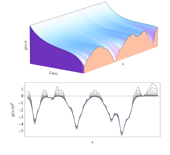
We have studied the SBR equation in 3D numerically solving for $g(x,t)$ at given $s(x)$ and verified that the above description remains essentially valid. In particular both for negative and positive values of $\sigma$ the solution $g(x,t)$ escapes to minus infinity (i.e. leaves the plateau) at all points $x$. This corrects a disturbing pathology of the simplified SBR equations where there are always regions that remains blocked near the plateau and never decay. More precisely $g(x,t)$ exits from the plateau with the very same Von-Schweidler law with a space dependent constant $B(x)$, (see fig. 1 )

$$g(x,t)\sim-B_{\sigma}(x)t^{b}\ \ \ for\ all\ \sigma$$

Therefore at any value of $\sigma$ the SBR equations induce a non-trivial mapping between the realization of the fluctuations $s(x)$ and a positive function $B(x)$ (called $B$-profile in the following). In practice we extract the $B$-profile by solving the equations up to times large enough to be in the asymptotic regime where $g(x,t)\approx-B(x)t^{b}$. The presence of the gradient term in the full SBR equation leads to the disappearance of a clear distinction between liquid and glassy regions as all regions become liquid, nevertheless when we switch on the gradient the regions that were glassy will be characterized by a very small value of $B(x)$ compared to the rare liquid regions where $B(x)$ is relatively much larger. The $B$-profile will be our main focus in the following, indeed it allows a discussion in a clear and compact way of many dynamical quantities including the $\alpha$-relaxation time, diffusion coefficient, correlation length and Dynamical Heterogeneities.

It is illuminating to directly inspect the $B$-profile above and below the critical temperature.

In figure (2) we plot the normalized $B$-profile $B(x)/\overline{B}$ on a plane sliced from a cubic box. The peaks(valleys) in the $B$-profile correspond to regions that are decorrelating from the initial condition faster(slower) than the average and where local dynamics is also faster(slower). The height and size of the peaks allows to characterize dynamical fluctuations. We see that for $T\geq T_{c}$ ( i.e. $\sigma\leq 0$) fluctuations are not very pronounced and the system appear homogeneous, instead below $T_{c}$ more and more peaks disappear and as a consequence the few that are left tend to be much more pronounced. Overall the average value $\overline{B}$ decrease monotonically with decreasing the temperature (it changes by orders of magnitude for the values of $\sigma$ of the plot) but the dynamics becomes instead dominated by rare regions that are relatively much faster than the typical region. Thus the evolution of the $B$-profile encodes a qualitative change in the structure of dynamical fluctuations marked by the appearance of Dynamical Heterogeneities at the crossover temperature. On the other hand one can immediately see that the size of the peaks does not change significantly above and below $T_{c}$. In the following sections we will analyze the $B$-profile more carefully and we will see in particular that the correlation length is actually slightly decreasing below $T_{c}$.

The viscosity $\eta$ and the diffusivity $D$ can be associated to different averages of the $B$-profile. Following the same matching arguments valid in MCT we can associate the $\alpha$ time scale to the coefficient of $t^{b}$ in the total correlator $G(t)$, this leads naturally to:

$$\eta=\tau_{\alpha}\sim\left({1\over V}\int B(x)\,dx\right)^{-1/b}$$

(7)

On the other hand, as discussed in [3], within SBR it is natural to consider a local relaxation time $\tau_{\alpha}(x)\sim B(x)^{-1/b}$ defined as the time scale where $-B(x)t^{b}$ is $O(1)$. One would therefore associate the diffusivity to the inverse of this local relaxation time:

$$D\sim{1\over V}\int B^{1/b}(x)\,dx$$

(8)

In figure (3) we plot $\tau_{\alpha}$ and $D$ as a function of $\sigma$ together with exemplary experimental data, obtained by Schneider et al. [7, 8] from dielectric spectroscopy on propylene carbonate. The behavior of this quantities is similar to what has been found in the simplified model. Let us make a few comments on the figure:

• •

  the divergence of $\tau_{\alpha}$ at $\sigma=0$ of ideal MCT is avoided but the growth rate changes from power-law to a more pronounced exponential-like growth: $T_{c}$ is avoided but marks a crossover.

• •

  The above property should be assessed remembering that there is no ad hoc assumption on activation processes in the derivation of SBR, rather the initial assumption is i.e. that $T_{c}$ marks a genuine phase transition.

• •

  The comparison with the data show that the description provided by SBR could work in an extended range of temperature, although it depends on a few number of parameters.

• •

  Used as fit functions the SBR expressions for $D$ and $\eta$ could help reconcile different estimates of $T_{c}$ based on asymptotic behavior.

• •

  SBR leads to an apparent shift of $T_{c}$ to lower values when fitted with ideal MCT power laws and this could provide an explanation of the well-known shift of the quantitative prediction of $MCT$ with respect to simulation data [1], see fig. (4).

• •

  In the figure the SBR expression for the $\tau_{\alpha}$ was used essentially as a fit function to the data but the actual computation of the parameters $\Delta\sigma$ and $\alpha$ is feasible for many systems that can be simulated numerically. These computations are left for future work.

As a technical remark we note that at given value of $\lambda$ the SBR equations depend in principle on three parameters $\alpha$, $\sigma$ and $\Delta\sigma$. However it suffices to solve it for fixed values of two of them. The natural way to do that is to consider fixed values of $\Delta\sigma$ and $\alpha$ and vary $\sigma$. The general solution can then be obtained from the reference solution by means of appropriate rescalings. The numerical data shown here correspond to the following choice of the parameters:

$$\alpha=.2\,,\,\Delta\sigma=.1,\,\lambda=.75\ ,$$

(9)

The spatial fluctuations of the dynamics in the late $\beta$ regime are conveniently encoded by the spatial fluctuations of the $B$-profile. We introduce the self-correlation of the $B$-profile as:

$$\Gamma(r)\equiv{1\over V}\int B(x)B(x+r)\,dx$$

(10)

The numerical solution shows that while the absolute value of $\Gamma(r)$ changes by orders of magnitude upon crossing $\sigma=0$ (it is related to $\tau_{\alpha}$), its shape and length-scale vary much less. In order to focus solely on the space dependence we introduce the normalized self-correlation:

$$\Gamma_{n}(r)\equiv\frac{\Gamma(r)-\Gamma(\infty)}{\Gamma(0)-\Gamma(\infty)}$$

(11)

We observe that in 3D $\Gamma_{n}(r)$ has a bell-shaped form with rapidly decaying tails both below and above $\sigma=0$. Quite interestingly it turns out that the width of $\Gamma_{n}(r)$ has a non-monotonous behavior with $\sigma$: in the bottom of figure (3) we plot the half-width at half-maximum of $\Gamma_{n}(r)$ as a function of $\sigma$ and use it as a definition of the dynamical correlation length. The figure demonstrates what we anticipated in the introduction: the dynamical correlation length increases approaching $\sigma=0$ from the liquid phase, it saturates to a maximum at $\sigma=\sigma_{max}$ slightly below $T_{c}$ and then it decreases again. In the same region the relaxation time increases instead by orders of magnitude implying that near $\sigma=0$ the correlation length decouples from the relaxation time. For instance considering the interval $\sigma=[-.01,.015]$ the correlation length increases and decreases again with an approximate $25\%$ excursion while the relaxation time increases by almost $8$ orders of magnitude.

It is tempting to put these results in connection with recent observations of non-monotonous correlation lengths in numerical simulations [9] and experiments [10]. These observations however should be contrasted with recent measurements [11, 12] of dynamical correlation lengths for the same systems obtained with the more standard methods of Refs. [13, 14, 15, 16]. In this case a monotonous behavior was instead observed, albeit displaying evidences of saturation towards a maximum [11, 12]. With regard to this open issue we note that, as discussed in [2], SBR is valid as it is near the crossover region. In particular the assumption that the separation parameter $\sigma$ is the sole temperature-dependent quantity (a typical assumption for a genuine phase transition) could be too strong well below $T_{c}$. On the other hand according to fig. (3) the correlation length does not change too much with the temperature, and one cannot exclude the possibility that the temperature dependence of the parameters $\alpha$ and $\Delta\sigma$ alters the non-monotonous behavior in actual systems. Qualitatively however the scenario of fig. (2) would remain the same: the amplitude of fluctuations (the height of the peaks) increase considerably while their size does not change significantly and this should be considered the essential feature of SBR independently on weather this size is actually increasing or decreasing.

Given that the correlation length displays a symmetrically decrease far away from $T_{c}$ both above and below one may ask what is actually happening at the crossover. As we saw before the answer is that there is a dramatic change in the structure of dynamical fluctuations above and below the crossover temperature as can be seen by direct inspection of the $B$-profiles. Let us now examine figure (2) thoroughly. We can distinguish two regimes above and below the crossover temperature. Above the critical temperature ($\sigma<0$) the normalized $B$-profile has fluctuations of order $O(1)$ around its average value which is one by definition. The profile is characterized by peaks whose width is of the order of magnitude of the correlation length. Increasing $\sigma$ towards $\sigma=0$ the profile does not change much, although we observe slightly larger fluctuations in the height of the peaks. In this regime the profile evolves much as in a second-order phase transition: the correlation length increases and so do the amplitude fluctuations. Here the correlation length carries relevant information: the system is essentially scale-invariant in the sense that the profiles at different values of $\sigma\leq 0$ look the same once space is rescaled proportionally to the correlation length. However at higher values of $\sigma$ ($\sigma=.006$) the $B$-profile starts to change qualitatively: the height of the typical region decreases as more and more of the lowest peaks disappear, conversely the few peaks left increase their relative height because they carry all the weight. As a result at $\sigma=.012$ we have a completely different landscape characterized by rare regions where the dynamics is relatively much faster ($B(x)/\overline{B}\gg 1$ at the peaks) then the surrounding slowly-moving regions ($B(x)/\overline{B}\ll 1$ in the typical region). Quantitatively we see that while fluctuations are $O(1)$ at $\sigma=-.006$, for $\sigma=0.012$ the normalized $B$-profile is $2-3$ orders of magnitude larger in the rare fast regions with respect to the neighboring slow regions. From figure (2) we also see that the size and shape of the peaks does not change much, which result in the fact that the correlation length does not change significantly for the values of $\sigma$ considered (as seen in figure (3)).

These features suggest that we should consider carefully the role of the correlation length at the glass crossover and the very same notion of Dynamical Heterogeneity (DH). Although dynamical fluctuations grow in both regimes they have power-law increase and remains relatively small in the first regime while they grow significantly in the second regime where they have essentially an activated nature. Therefore only in the second regime we should actually talk of Dynamical Heterogeneities as defined from experiments [17] and as a consequence we should conclude that within SBR DH are not intrinsically associated with an increasing correlation length.

It is to be expected that the qualitative change in the structure of the dynamical fluctuations from scale-invariant-like to activated-like can be detected by comparing observables that are associated to different averages of $B(x)$. In figure (5) we plot parametrically the viscosity and the diffusivity computed according to expressions (7) and (8). They obey the Stokes-Einstein relationship (SER) $D\eta\propto 1$ for temperatures above $T_{c}$, while below the crossover (the black dot) there is a violation of the SER. Once again this is a typical feature of glassy systems as the exemplary data demonstrates.

References

- [1] W. Götze, Complex Dynamics of Glass-Forming Liquids (Oxford University Press, Oxford, 2009).
- [2] T. Rizzo, EPL (Europhysics Letters) 106, 56003 (2014).
- [3] T. Rizzo and T. Voigtmann, (2014), arXiv:1403.2764 .
- [4] G. Biroli, J.-P. Bouchaud, K. Miyazaki, and D. R. Reichman, Phys. Rev. Lett. 97, 195701 (2006).
- [5] S. Franz, H. Jacquin, G. Parisi, P. Urbani, and F. Zamponi, Proceedings of the National Academy of Sciences 109, 18725 (2012), http://www.pnas.org/content/109/46/18725.full.pdf+html .
- [6] T. Rizzo, (2013), arXiv:1307.4303 .
- [7] U. Schneider, P. Lunkenheimer, R. Brand, and A. Loidl, Phys. Rev. E 59, 6924 (1999).
- [8] P. Lunkenheimer, U. Schneider, R. Brand, and A. Loidl, Contemp. Phys. 41, 15 (2000).
- [9] W. Kob, S. Roldán-Vargas, and L. Berthier, Nature Physics 8, 164 (2012).
- [10] K. H. Nagamanasa, S. Gokhale, A. Sood, and R. Ganapathy, arXiv preprint arXiv:1408.5485 (2014).
- [11] E. Flenner and G. Szamel, Nature Physics 8, 696 (2012).
- [12] E. Flenner and G. Szamel, J. Chem. Phys. 138, 12A523 (2013).
- [13] S. Franz, C. Donati, G. Parisi, and S. C. Glotzer, Philosophical Magazine B 79, 1827 (1999).
- [14] C. Donati, S. Franz, S. C. Glotzer, and G. Parisi, Journal of non-crystalline solids 307, 215 (2002).
- [15] N. Lačević, F. W. Starr, T. Schrøder, V. Novikov, and S. Glotzer, Physical Review E 66, 030101 (2002).
- [16] N. Lačević, F. W. Starr, T. Schrøder, and S. Glotzer, The Journal of chemical physics 119, 7372 (2003).
- [17] M. D. Ediger, Annu. Rev. Phys. Chem. 51, 99 (2000).
- [18] M. Lohfink and H. Sillescu, AIP Conf. Proc. 256, 30 (1992).
- [19] T. R. Kirkpatrick and D. Thirumalai, Phys. Rev. B 36, 5388 (1987a).
- [20] T. R. Kirkpatrick and D. Thirumalai, Phys. Rev. Lett. 58, 2091 (1987b).
- [21] T. R. Kirkpatrick and P. G. Wolynes, Phys. Rev. B 36, 8552 (1987).
- [22] S. Franz, G. Parisi, F. Ricci-Tersenghi, and T. Rizzo, The European Physical Journal E 34, 1 (2011).
- [23] T. R. Kirkpatrick, D. Thirumalai, and P. G. Wolynes, Phys. Rev. A 40, 1045 (1989).
- [24] C. Dalle-Ferrier, C. Thibierge, C. Alba-Simionesco, L. Berthier, G. Biroli, J.-P. Bouchaud, F. Ladieu, D. L’Hôte, and G. Tarjus, Phys. Rev. E 76, 041510 (2007).
- [25] L. Berthier, G. Biroli, J.-P. Bouchaud, L. Cipelletti, D. El Masri, D. L’Hôte, F. Ladieu, and M. Pierno, Science 310, 1797 (2005).
- [26] C. Crauste-Thibierge, C. Brun, F. Ladieu, D. L’Hôte, G. Biroli, and J.-P. Bouchaud, Phys. Rev. Lett. 104, 165703 (2010).
- [27] Th. Bauer, P. Lunkenheimer, and A. Loidl, Phys. Rev. Lett. 111, 225702 (2013).