The Best Constraints on A Super-Eddington Accretion Flow: XMM-Newton Observations of An Intermediate-mass Black Hole
Abstract
RX J1140.1+0307 (hereafter RX1140) is a Narrow Line Seyfert 1 (NLS1) with one of the lowest black hole masses known in an AGN (M M☉). We show results from two new XMM-Newton observations, showing soft 2-10 keV spectra, a strong excess at lower energies, and fast X-ray variability as is typical of this class. The soft excess can be equally well fit by either low temperature Comptonisation or highly smeared, ionised reflection models, but we use a covariance analysis of the fast X-ray variability as well as lag and coherence spectra to show that the low temperature Comptonisation model gives a better description of the break in variability properties between soft and hard X-rays. Both models also require an additional component at the softest energies, as expected from the accretion disc. However, this inner disc spectrum does not join smoothly onto the variable optical and far UV emission (which should be produced in the outer disc) unless the mass is underestimated by an order of magnitude. The variable optical and far UV emission instead suggests that through the outer disc, in which case advection and/or wind losses are required to explain the observed broadband spectral energy distribution. However, the similarity of the X-ray properties of RX1140 to other simple NLS1 such as PG 1244+026, RE J1034+396 and RX J0136 means it is likely that these are also super-Eddington sources. This means their spectral energy distribution cannot be used to determine black hole spin despite appearing to be disc dominated. It also means that the accretion geometry close to the black hole is unlikely to be a flat disc as assumed in the new X-ray reverberation mapping techniques.
Keywords:
accretion, Eddington ratio, variability, active-galaxies: nuclei1 Introduction
Intermediate mass black holes (IMBH), which are taken to refer to masses from , are of particular interest because this population would fall within the gap between the two principal black hole populations, i.e. super-massive black holes (SMBH) with and stellar mass black holes with . Currently there are very few well studied IMBH, two examples are NGC 4395 (Filippenko & Ho 2003) and POX 52 (Kunth, Sargent & Bothun 1987; Barth et al. 2004).
For over two decades, the most robust technique to measure black hole masses in Active Galactic Nuclei (AGN) has been the reverberation mapping (RM) technique, which estimates the radius of the broad line region (BLR) by measuring the time-lag between the line emission from the BLR and the intrinsic continuum emission from the accretion disc. Since optical RM requires well sampled spectroscopical monitoring of variable AGN for months or years, the total number of sources with RM masses is currently less than forty (e.g. Kaspi et al. 2000; Peterson et al. 2004, 2005; Denney et al. 2006, Bentz et al. 2009b; Du et al. 2014). Instead, the RM measurements can be used to derive a radius-luminosity relation which can then give black hole mass from single epoch measurements using the Balmer line width (normally that of H FWHM) and luminosity (generally monochromatic luminosity at 5100Å, hereafter e.g. Bentz et al. 2006, 2009a; Denney et al. 2010). Employing this method, Greene & Ho (2004) identified 19 IMBH in the SDSS database. Later on Dong et al. (2007) and Greene & Ho (2007) extended the IMBH sample to include several hundred sources.
RX J1140.1+0307 (hereafter RX1140), also referred to as GH 08 or SDSS J114008.71+030711.4, is amongst the original 19 IMBH sample of Greene & Ho (2004). It has a redshift of 0.081 (co-moving distance of 336 Mpc). The SDSS and HST images show a resolved disc component, plus a bar and AGN components (Greene, Ho & Barth 2008). The H FWHM measured from the SDSS spectrum is (Ai et al. 2011; Jin et al. 2012a). However, to get mass also requires , and this is made more difficult by the strong host galaxy contamination. Deconvolution of the HST image gives an estimated AGN continuum of , which is somewhat smaller than the observed variable flux of (Rafter et al. 2011). This gives a black hole mass of (Greene, Ho & Barth 2008; Ai et al. 2011). However, Rafter et al. (2011) applied the RM technique to RX1140, and reported an upper limit of 6 light days for , which gives , but this is probably too strict a limit given that their average sampling time of 6.1 days. A more conservative upper limit from the reverberation is probably a factor 2 larger, giving , consistent with the mass estimate.
For this small a black hole mass, the total AGN luminosity is likely to be a high fraction of Eddington, with Zhang & Wang (2006) estimating from (though using the luminosity corrected for host galaxy contamination reduces it to ). So far, such high Eddington fraction accretion flows, with , are found in the subset of broad line AGN known as Narrow-Line Seyfert 1 (e.g. Osterbrock & Pogge 1985; Boroson & Green 1992; Leighly 1999). Their narrow Balmer lines indicate relatively small black hole masses (: Boroson 2002), so that their bolometric luminosities are close to Eddington. For such high Eddington fractions it is clearly a moot point as to whether the H scaling relations hold. Marconi et al. (2009) suggest a correction to the mass scalings such that the BLR clouds trace the effective gravity, but the lack of observed wind features in the low ionisation BLR lines form a strong argument against such effects being important. This could indicate that the clouds are optically thick to electron scattering, with columns of cm-2, or that the radiative acceleration only affects the front face of the cloud (Baskin, Laor & Stern 2014). Thus it seems probable that the H line widths reflect the black hole mass even at Eddington and potentially beyond.
One of the ubiquitous features of high Eddington fraction AGN is their prominent soft X-ray excess superposed on a steep X-ray power law which is very variable. These properties are seen in the X-ray spectrum of RX1140 (Miniutti et al. 2009; Ai et al. 2011). While the variability scales with black hole mass, making it unsurprising that the X-ray variability of RX1140 is amongst the strongest seen AGN (e.g. Ponti et al. 2012; Ludlam et al. 2015), the origin of the soft excess is more puzzling. Models which reproduce the shape include optically thick, low temperature Comptonisation (e.g. Laor et al. 1997; Magdziarz et al. 1998; Gierliński & Done 2004; Jin et al. 2013), ionised, highly smeared reflection (e.g. Fabian & Miniutti 2005; Zoghbi et al. 2010; Fabian et al. 2013; Fabian, Kara & Parker 2014; Uttley et al. 2014), and smeared absorption (Gierliński & Done 2004; 2006). The smeared absorption model is disfavoured on theoretical (Schurch & Done 2007) as well as observational grounds (Miniutti et al. 2009, Ai et al. 2011), but both Comptonisation and smeared reflection provide a good fit to the soft excess in this object (Ai et al. 2011).
However, for such low mass, high mass accretion rate AGN, the disc itself should also contribute a significant fraction of the emission in the soft X-ray bandpass. It is well known that the accretion flow spectrum is not well described by a disc in standard broad line Seyfert 1s and Quasars (e.g. Elvis et al. 1994), but the higher Eddington ratio NLS1 have spectra which do appear to be more disc-dominated (Jin et al. 2012a,c; hereafter J12a; c; Done et al. 2012, hereafter D12). This is most easily seen in the context of the full Spectral Energy Distribution (SED) as the optical/UV disc normalisation is determined by the product of mass and mass accretion rate, with . Thus this directly measures mass accretion rate if the black hole mass is known, and hence the total luminosity , where the efficiency depends on black hole spin (e.g. Davis & Laor 2011; Done et al. 2013). This also predicts where the disc disc emission peaks, and show that the disc spectrum should extend into the soft X-ray bandpass for the NLS1 even at low spin (Done et al. 2013).
RX1140 is the lowest mass NLS1 included in the sample of 51 unobscured Type 1 AGN of J12a,c. These papers carried out a detailed study of the broadband SED from optical to hard X-rays, fitting them with the new accretion models which allow some of the accretion energy to be dissipated in a Comptonised soft X-ray excess and power law tail as well as in the thin disc (D12). These assume energy conservation i.e. that there is no strong energy loss via advection and/or winds as might be expected in highly super-Eddington sources. J12a, c used the black hole mass was a fit parameter within the uncertainties derived from using the intermediate and broad H line component widths as lower and upper limits, respectively. This gave a best fit value of for this source (J12a), which increased to when the updated SED models including a colour temperature correction to the disc emission were used (D12, J12c). Clearly the mass of RX1140 derived from broadband SED fitting is much higher than the virial and RM mass estimates, and this requires further consideration.
The X-ray properties of RX1140 are very similar to a small group of the most extreme NLS1s, such as PG 1244+026, RE J1034+396 and RX J0136.9-3510, which all exhibit strong X-ray variability, prominent and featureless soft excesses and are all reported to be accreting around the Eddington limit (Middleton et al. 2009; Jin et al. 2009; Jin et al. 2013). In order to investigate the physical interpretation for the soft excess seen in RX1140, a detailed timing analysis must be performed in conjunction with the spectral analysis (e.g. Jin et al. 2013). In achieve this we applied for a long XMM-Newton observation for this source. This was successful, but was split into two observations separated by two weeks. In this paper we present the results from a combined analysis of these two newXMM-Newton observations, plus the previous one extracted from the archive.
This paper is organised as follows: Section 2 describes the data reduction procedures used for the XMM-Newton observations. Section 3 presents variability properties of RX1140. Section 4 presents a combined spectral and variability study of the target. We compare two physical models for explaining the properties of the 0.3-10 keV spectra and variability. In Section 5, we perform broadband SED fitting by including ultraviolet (UV), optical and near-infrared data. In section 6 we discuss issues such as various estimates of the black hole mass, UV/optical luminosity and the mechanism responsible for the soft X-ray excess. Our summary and conclusions are given in section 7. When converting flux to luminosity, we adopt a flat universe model with the Hubble constant H km s-1 Mpc-1, and .
2 Data Reduction
RX1140 was observed by the XMM-Newton satellite on 3rd, Dec., 2005 (Principal Investigator: Dr. Giovanni Miniutti) (hereafter: Obs-1). We proposed a longer observation with the aim to study its X-ray variability. Our observation was divided into two parts due to satellite scheduling. These were carried out on 18th, Dec., 2013 (hereafter: Obs-2) and 1st, Jan., 2014 (hereafter: Obs-3). During the three observations, all EPIC cameras were in the full window mode. We used SAS v13.5.0 and the latest calibration files, and followed the standard procedures to reduce the data. We chose the source extraction region to be a circular region of radius 45″for each EPIC camera. The background was selected from a nearby circular region with the same radius as for the source. For Obs-1 the net source count rates are , and for the PN, MOS1 and MOS2, respectively. Obs-2 has a mean count rate that is half that of Obs-1. Obs-3 has a similar mean count rate as Obs-1. All of these count rates are well below the threshold count rates capable of causing a photon pile-up effect in the full window mode of each EPIC camera.
We selected data with PATTERN 12 for MOS1 and MOS2, and PATTERN 4 for the PN. Light curves were extracted from both the source and background regions. There were high background flares in all three observations. Therefore we visually checked the background light curves to identify high background sections and removed them. Then the background was subtracted from the source light curve using LCMATH in FTOOLS. Spectra were extracted for the source and background regions, separately. Response matrices were produced using RMFGEN and ARFGEN. Areas for the source and background regions were calculated using BACKSCALE. We also used the SAS task RGSPROC to extract the 1st order spectra from RGS1 and RGS2. Response matrices for the RGS were produced with RGSRMFGEN. All spectra were rebinned by GRPPHA with a minimum of 25 counts per bin, so that the fitting is appropriate.But the signal-to-noise of RGS spectra are too low to provide further information, so we do not present them in this paper. All spectral fittings were performed in xspec v12.8.2 (Arnaud 1996).
There are also simultaneous Optical/UV observations obtained using the XMM-Newton Optical Monitor (OM). OBs-1 has UVW1 and UVM2 filter data, while Obs-2 and 3 have U, B and UVW1. We searched the OM source list file to obtain the count rate of RX1140, in each available filter, and inserted these values into the standard OM data file template om_filter_default.pi. The data file was then combined with the ‘canned’ response files11 1 http://heasarc.gsfc.nasa.gov/FTP/xmm/data/responses/om to be ready for xspec fitting.
3 Variability Study
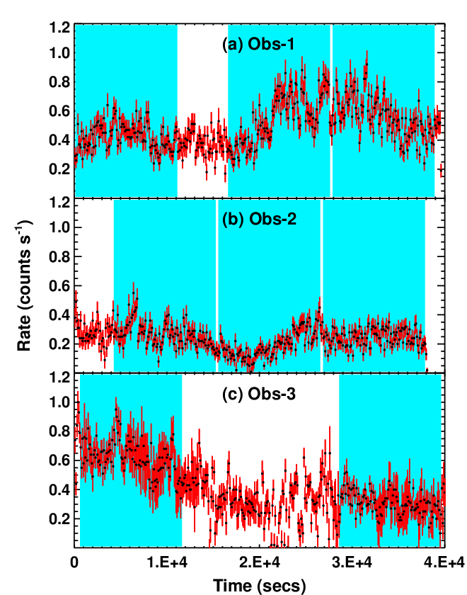
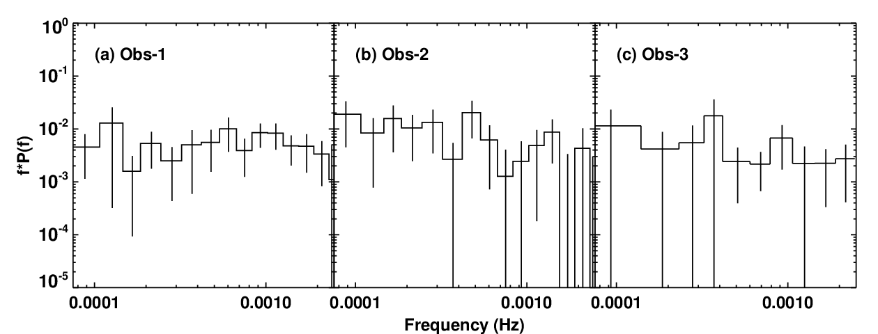
The background subtracted PN light curves over the total energy band (0.3-10 keV) are shown in Figure 1. Strong variability is observed over all timescales. This is also confirmed by their Power Spectral Density (PSD) in Figure 2. The flat PSD indicate that intrinsic variability (i.e. Poisson noise subtracted) exists throughout the 0.2-10 ks timescale. None of the observations show any sign of a high frequency break. This is clearly different to the case of PG 1244+026, where the 0.3-1 keV power spectrum drops substantially above Hz (Jin et al. 2013), thus strongly suggests that RX1140 is substantially lower mass than PG 1244+026, and that the mass is (Ponti et al. 2012; Kelly et al. 2013; Ludlam et al. 2015).
The time-averaged X-ray spectra for Obs-1 (black) and Obs-2 (red) are shown in the upper panel of Figure 3. The mean spectrum of Obs-3 is almost identical to Obs-1, so it is not shown in the figure. The Obs-1 and Obs-2 spectra are quite similar, but a ratio of the best fit model to Obs-1 (black solid model), rescaled to the observed 2-10 keV spectrum of Obs-2 (red solid model) under-predicts the soft emission. This longer term (weeks to years) variability can be compared to the rapid variability. The shapes of high (: orange) and low (: blue) count rate spectra from Obs-1 are identical within errors to the mean spectrum. This can be seen in the lower panel of Figure 3, which gives the ratio of each dataset to the mean spectral model renormalised to the 2-10 keV count rate.
3.1 RMS Spectra
Fractional variability observed in different energy bins, i.e. the RMS spectra (e.g. Edelson et al. 2002; Markowitz, Edelson & Vaughan 2003; Vaughan et al. 2003), can be very useful in decomposing the different spectral components. We use the segment algorithm detailed in Wilkinson & Uttley (2009) to calculate the RMS. For every energy bin, the light curve is divided evenly into several segments. Then the excess variance is calculated for every segment and averaged over all segments. The square-root of the excess variance is RMS. The error-bars are calculated using Equation B2 in Vaughan et al. (2003). The binning time and segment length determine the timescale for which the RMS is calculated. The high background intervals interrupt the continuity of the light curve. In Obs-3, the longest continuously sampled segment is only 11 ks, while it is longer in Obs-1 and Obs-2. To mitigate bias from high background contamination, we choose a longest segment length of 11 ks, and so are able to identify a total of eight segments with little high background, i.e. three segments in Obs-1, three in Obs-2 and two in Obs-3 (see the cyan regions in Figure 1).
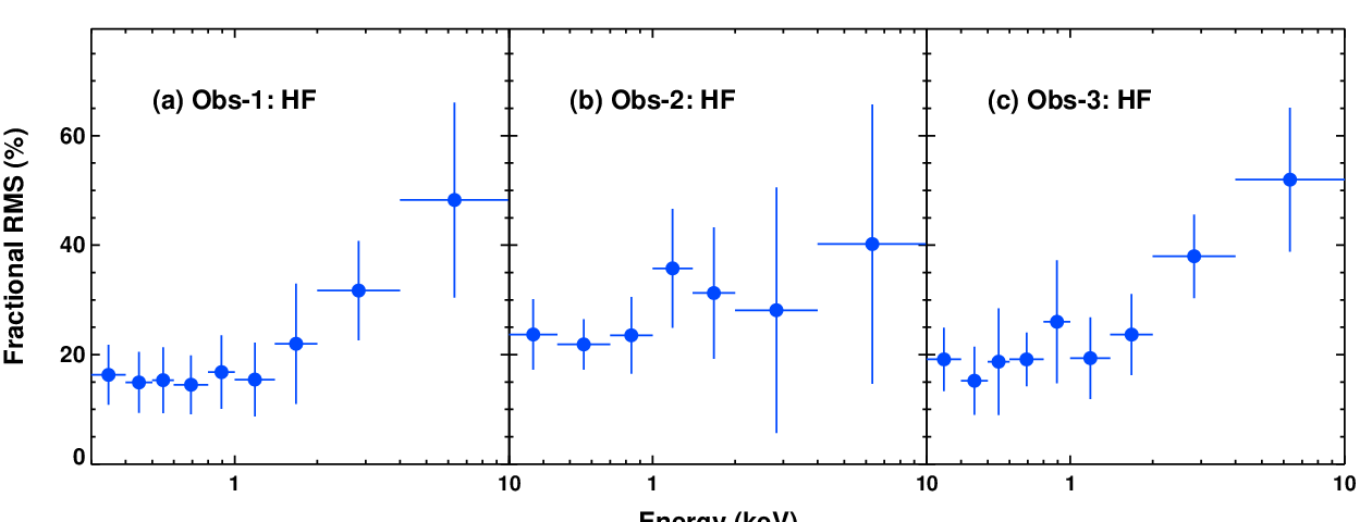
There are insufficient data to produce frequency-resolved RMS spectra. Instead, we calculate only RMS of the highest frequency (HF) variability using timescales of 0.2-2 ks from the eight 11ks segments. The results are shown in Figure 4. Interestingly, the HF RMS spectra reveal a rising shape from soft to hard X-ray ranges in Obs-1 and Obs-3, which is similar to that observed in some other high mass accretion rate NLS1s, such as PG 1244+026 (Jin et al. 2013), RE J1034+396 (Middleton et al. 2009) and RX J0136.9-3510 (Jin et al. 2009). This difference in variance between soft and hard energy bands can be easily explained if the soft X-ray excess varies less than the power law tail, favouring models where this is a true additional component e.g. from soft Comptonisation (e.g. Gierliński & Done 2004, Middleton et al. 2009, Jin et al. 2013, Matt et al. 2014) rather than due to ionised, smeared reflection, as this tends to contribute equally in soft and hard bands (Gierliński & Done 2006).
Another key feature seen in Figure 4 is that the 0.3-1 keV HF RMS in Obs-2 is rather different to that of Obs-1 and Obs-3, with much less difference between the fast variability as a function of energy (more HF power below 1 keV, and marginally less at the highest energies). Whatever happened to depress the soft spectrum relative to the mean (Figure 3) may also increased its fast variability (see Gardner & Done 2015 for a possible explanation of this in terms of cloud occultions in the inner disc).

3.2 Covariance spectra
The RMS variability spectrum shows all variability at each energy, but where there may be multiple components. A more powerful technique is the covariance spectrum (developed by Wilkinson & Uttley 2009) as it determines the spectrum of the variability correlated with a given energy band lightcurve used as a reference. For the NLS1 PG 1244+026, Jin et al. (2013) showed that using the fastest variability in the hard X-ray (2-10 keV) lightcurve as a reference band gave strong evidence for a Comptonisation origin for the soft X-ray excess, while using the fastest variability in the 0.3-1 keV band showed evidence for a contribution at the lowest energies from the disc.
Here we apply the same technique to our datasets to produce the HF (0.2-2 ks) covariance spectra using hard (2-10 keV) and soft (0.3-1 keV) X-rays as the reference band. We use only PN data so as not to have differences in response from combining PN and MOS. But the data quality means that the signal-to-noise of the covariance spectra for RX1140 is much lower than for PG 1244+026. Then we study both the covariance spectra and the time-averaged spectrum (see Figure 5) in order to try to determine the origin of the soft X-ray excess, i.e. whether it can be better fit by an additional Comptonisation model or by relativistically smeared reflection, and whether there is also a contribution from the accretion disc itself.
4 Spectral Analysis
The X-ray spectrum derived from Obs-1 has been analysed previously. Miniutti et al. (2009) found that an X-ray reflection plus a thermal disc model, gives a better fit than the smeared absorption model. Ai et al. (2011) found that reflection and Comptonisation models gave comparably good fits, and that both these were better than smeared absorption and -free disk models. The shape of the HF RMS and mean spectra in Figure 3 and Figure 4 also indicates that RX1140 may be similar to other extreme NLS1s such as PG 1244+026, RE J1034+396 and RX J0136.9-3510, whose soft X-ray excess can be well interpreted by Comptonisation model. Therefore, we try both Comptonisation and reflection models for Obs-1 and Obs-2 spectra. The best-fit models are shown in Figure 5.
 |
 |
 |
 |
4.1 Comptonisation Model
For the Comptonisation scenario, we use a low temperature, optically thick Comptonisation model (comptt model, Titarchuk 1994; Hua & Titarchuk, 1995; Titarchuk & Lyubarskij 1995) to fit the soft X-ray excess; a high temperature Comptonisation (nthcomp model in xspec, Zdziarski, Johnson & Magdziarz 1996; Życki, Done & Smith 1999) to fit the power law tail, together with its neutral, smeared reflection (kdblur*pexmon, Laor 1991; recoded as a convolution model, Nandra et al. 2007). We also include an accretion disc component (diskbb model, Mitsuda et al. 1984; Makishima et al. 1986). Using the equation in Peterson (1997) and assuming , and (Miniutti et al. 2009), we calculate the temperature at the inner radius (Tin) to be 110 eV. Including a colour temperature correction would increase this, while allowing the some of the inner disc power to be dissipated in powering the soft and hard X-ray Compton components would decrease it, so we freeze the parameter Tin at this temperature. It also serves as the temperature of the seed photons for both soft and hard X-ray Comptonisation components. We fix the Galactic column at (Kalberla et al. 2005) but allow additional free absorption by the host galaxy gas column (zwabs, Morrison & McCammon 1983). The complete xspec model parameters are given in Table 1.
The HF variability is likely to originate mainly from the inner region of the flow, where the hard X-ray emission is produced. Hence we expect that the spectrum correlated with the HF 2-10 keV variability should have the same shape as the high temperature Comptonisation component which dominates the 2-10 keV spectrum in this model. However, reflection (and associated thermal reprocessing which could contribute to the soft X-ray excess: Gardner & Done 2015a) should also vary in a correlated manner as the expected reverberation timescale (Fabian et al. 2009) is short for a low mass black hole. Only the disc is not expected to have any variability on these timescales.
| Model Name | Model Expression in xspec v12.8.2 | |||
| Comptonisation | CONSTANT*WABS*ZWABS*( DISKBB+ NTHCOMP + COMPTT + KDBLUR*PEXMON ) | |||
| Spectrum | Component | Parameter | Value | Value |
| Obs-1 | Obs-2 | |||
| Mean Spec | ZWABS | NH (1022 ) | 0 | 0.027 |
| DISKBB | Tin (keV) | 0.11 fixed | 0.11 fixed | |
| DISKBB | norm | 135 | 135 fixed | |
| NTHCOMP | 2.26 fixed | 2.26 fixed | ||
| NTHCOMP | kTseed (keV) | tied to Tin | tied to Tin | |
| NTHCOMP | kTe (keV) | 100 fixed | 100 fixed | |
| NTHCOMP | norm | (1.26 ) | (8.11 ) | |
| COMPTT | kTseed (keV) | tied to Tin | tied to Tin | |
| COMPTT | kT (keV) | 0.38 | 0.21 | |
| COMPTT | 10.9 | 19.2 | ||
| COMPTT | norm | (2.68 ) | (1.81 ) | |
| KDBLUR | Rin () | 20 fixed | 20 fixed | |
| PEXMON | Relrefl | -1.0 pegged | -1.0 pegged | |
| Cov. Spec | NTHCOMP | norm | (5.86 ) | (2.21 ) |
| COMPTT | norm | (1.45 ) | (9.74 ) | |
| Reflection | CONSTANT*WABS*ZWABS*( DISKBB + NTHCOMP + KDBLUR*RFXCONV*NTHCOMP ) | |||
| Spectrum | Component | Parameter | Value | Value |
| Obs-1 | Obs-2 | |||
| Mean Spec | ZWABS | NH (1022 ) | 0 | 0.006 |
| DISKBB | Tin (keV) | 0.11 fixed | 0.11 fixed | |
| DISKBB | norm | 211 | 83 | |
| NTHCOMP | 2.42 | 2.22 | ||
| NTHCOMP | norm | 5.72 | 3.60 | |
| KDBLUR | Index | 5 fixed | 5 fixed | |
| KDBLUR | Rin () | 4.98 | 3.05 | |
| RFXCONV | Relrefl | -2.19 | -2.29 | |
| RFXCONV | Feabund | 1.39 | 0.81 | |
| RFXCONV | log | 3.37 | 2.86 | |
| Cov. Spec | NTHCOMP | norm | 4.90 | 1.08 |
| RFXCONV | Relrefl | -0.28 | -2.60 | |
To perform spectral fitting, we first applied the spectral model to the entire 0.3-10 keV spectrum, but we found some parameters were not well constrained because of parameter degeneracy. Therefore we attempt to constrain the hard X-ray Comptonisation and neutral reflection components by applying them only to the 2-10 keV spectra of Obs-1 and Obs-2. The model fits the 2-10 keV spectra well (). The hard X-ray photon index () is found to be 2.260.12, the inner radius parameter (Rin) of is 20 with reflection solid angle fixed at unity. Removing the neutral reflection component leads to , but the fitting statistics is only slightly worse (). The low signal-to-noise in the hard X-ray band cannot constrain this reflection component well. Then we re-fit the model to the entire 0.3-10 keV band by fixing at 2.26 and Rin at 20, and all spectral components are better constrained then before. The best fit parameters are listed in Table 1.
In Obs-1, the HF covariance spectrum can be well fitted by the hard Comptonisation with , without significant contribution from a variable soft Comptonisation component. On the contrary, the HF covariance spectrum in Obs-2 is softer so requires more contribution from the soft Comptonisation (Figure 5a and Figure 5b). Neither covariance spectrum requires any disc component.
We can also test for the presence of an accretion disc component in the soft X-ray bandpass by removing the disc component from the model and then re-fitting the Obs-1 spectra. The electron temperature (kT) of the soft Comptonisation component increases from 0.38 keV to 0.46 keV, the optical depth () decreases from 10.9 to 7.1, the normalisation increases by 10%. However, increases from 0.94 to 0.98 (i.e. for the removal of 2 free parameters, which is only marginally significant). The significance increases if we consider only the 0.3-0.5 keV band, where increases from 1.22 to 1.33 after removing the disc component. Thus both the time average spectra and HF variability support the decomposition of the soft X-ray spectrum into at least two components, which we interpret here as a contribution from the accretion disc, and an additional low temperature Comptonisation. A high temperature Compton spectrum is required to reproduce the 2-10 keV spectrum.
 |
 |
 |
 |
4.2 Reflection Model
Ionised, strongly smeared disc reflection plus a thermal accretion disc component was previously reported to be a good model for the time-averaged Obs-1 spectrum of RX1140 (Miniutti et al. 2009, Ai et al. 2011). Thus we use diskbb+nthcomp+kdblur*nthcomp as our spectral model, with Tin of the disc component fixed at 110 eV as before. Figure 5c and Figure 5d shows this model applied to Obs-1 and Obs-2 respectively. Again, the low statistics mean that some parameters cannot be well constrained. We choose to fix the illumination index of the smeared reflection at , and fit for the inner disc radius. This is always small in this model, at , so any reverberation timescale should be short. Hence both the high temperature Comptonisation and its reflection should vary together. However, the relatively flat HF covariance spectrum in Obs-1 favours a less reflection component contribution than in the time averaged spectrum, while the softer HF covariance spectrum in Obs-2 favours a larger reflection contribution. But again the poor signal-to-noise means that this is not very significant (Table 1). Similar as in the Comptonisation scenario, accretion disc component is not detected in the HF covariance spectra.
4.3 Lag and coherence spectra
Both Comptonisation and reflection models for the soft X-ray excess can give comparably good fits to both the time averaged and HF covariance spectra. Both models also require that there is an additional soft component, which we interpret as the direct disc emission, at the softest energies.
We can also use spectral coherence and time lags to constrain the X-ray spectral mechanisms (e.g. McHardy et al. 2004; Fabian et al. 2009). However, the low count rate of RX1140 and the relatively short continuously sampled light curve segments (11 ks, see Section 3) mean that the statistics are limited. We calculate these as in Nowak et al. (1999), using only Obs-1 and 3 (since Obs-2 has a significantly different spectrum and variability). We choose low and high energy band with 0.3-0.7 keV and 1.8-2.5 keV so as to try to best isolate different spectral components whilst still having enough counts.
Figure 6a shows that there is a soft reverberation lag of s seen between the 0.3-0.7 keV and 1.8-2.5 keV light curves at a frequency of Hz. But the zero spectral coherence and the dominance of Poisson noise at this frequency means this lag can be artificial. However, there is a clear positive lag at the lowest frequencies (below Hz), where the soft leads the harder band. This lag is supported by the good spectral coherence between these bands up to Hz (Figure 6c and Figure 6d). Note that Poisson noise will not be an issue on such long timescales. Figure 6b) shows the energy spectrum of this long timescale soft lead, showing that there is a clear break between the time lags at low and high energy, although we do not have enough statistics at hard X-ray. This is not easily compatible with the reflection model shown in Figure 5b), where a single component dominates the spectrum from 0.4-10 keV.
Thus while the signal-to-noise is poor, these data provide marginal evidences in terms of spectral coherence and time-lag to support a model where the majority of the soft X-ray excess does not contribute to the 2-10 keV bandpass, favouring the low temperature Comptonisation origin over the reflection dominated model.
5 Broad band Spectral Energy Distribution
5.1 Multi-wavelength Data
As outlined in the introduction, RX1140 was reported as an IMBH, whose mass is estimated to be accreting at a high fraction of the Eddington limit. We construct a multi-wavelength SED based on non-simultaneous observations (Figure 7). We use the XMM-Newton PN spectrum from Obs-1 taken in 2005, together with archival data from the ROSAT PSPCB (1992-06-16) which we reduced using XSELECT v2.4b. The spectra were regrouped fixing a minimum of 25 counts per bin, and are in good agreement with the time-averaged PN XMM-Newton spectrum.
In the optical and UV band, there are simultaneous photometric points from XMM-Newton OM for Obs-1 (UVM2 and UVW1 filters) and Obs-2 and Obs-3 (UVW1, U and B filters). The UVW1 filter fluxes of Obs-1 and Obs-3 are very similar, so are their X-ray fluxes, so we use all OM data from these two observations (except for UVW1 since its waveband is already covered by the combination of UVM2, U and B filter bands). We do not use Obs-2 as it is clearly different in optical/UV as well as X-ray, with only 90% flux in UVW1, 84% in U and 99% in B compared to Obs-3. These are less suppressed than the X-ray flux (Obs2/Obs3 = 46% in 0.3-2 keV, 63% in 2-10 keV), indicating that the amplitude of UV/optical variability is less than that of the X-ray over variability timescales of weeks and years.
Other data points in Figure 7 include GALEX photometry (obs-date: 2007-03-22), SDSS ugriz photometry and fibre spectrum (obs-date: 2001-03-26), UKIDSS Petrosian magnitude of JYHK photometry (obs-date: 2008-04-21). The difference in the normalisation, especially that for the UKIDSS and SDSS fibre fluxes, is likely due to different aperture sizes.
5.2 Broadband SED Fitting
We use optxagnf in xspec v12.8.2, to fit the SED from the optical to hard X-ray energies (D12). This includes both intrinsic disc emission, together with low and high temperature Comptonisation, as favoured by the spectral fits in Section 4. An additional neutral reflection (kdblur*pexmon model, Laor 1991, recoded as a convolution model by Nandra et al. 2007) is added to fit the marginally rising shape above 4 keV. We fix the inclination of the reflector at , and fix the spectral index of the hard Comptonisation component at 2.26 (see Section 4). We correct for extinction by a Galactic column density of (Kalberla et al. 2005). We also allow for intrinsic extinction in the host galaxy. This gives a best fit around at z = 0.0811 (zwabs model, Morrison & McCammon 1983). Both Galactic and intrinsic reddening are assumed to follow the standard dust to gas conversion formula of (Bessell 1991) and modelled by redden and zredden model (Cardelli et al. 1989) in xspec.
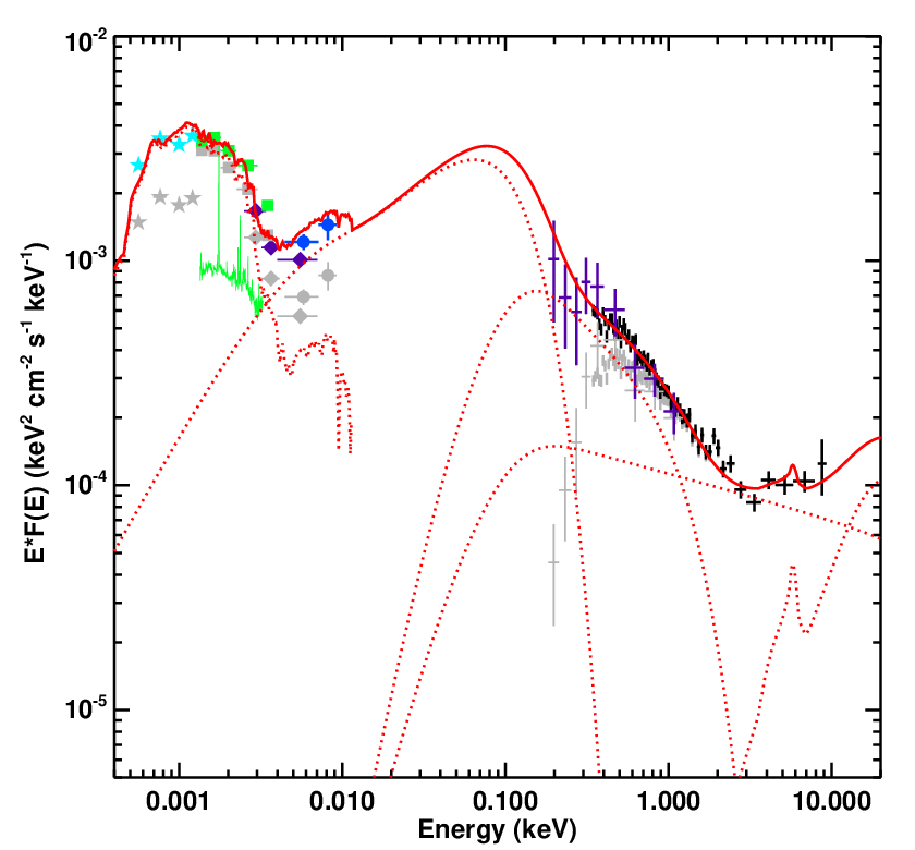
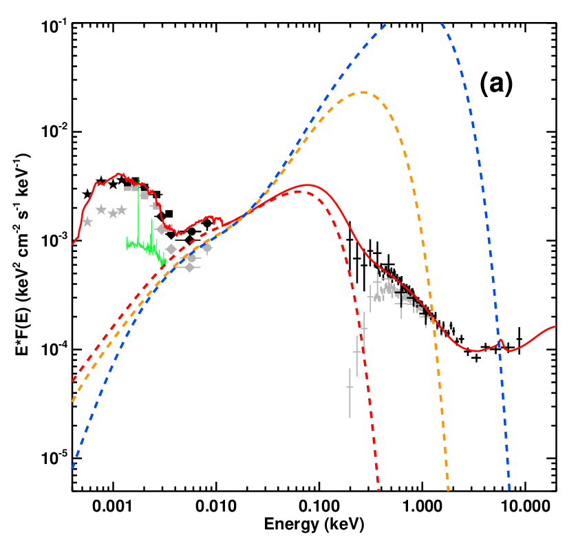
The far UV GALEX points fit nicely on the expected disc spectrum from optxagnf, but the optical and near UV points display a curvature similar to that of host galaxy emission. The SDSS images show that the host galaxy of RX1140 is of an Sc type galaxy. Therefore we select an Sc galaxy template from the SWIRE library (Polletta et al. 2007) and incorporate this into our xspec model. A constant normalisation offset is allowed between the UKIDSS points and other data.
Figure 7 shows the extinction/reddening/aperture corrected data (coloured points, compared to the observed data points in grey) and the best-fit SED model. The formal fitting statistics are poor (reduced ), which is mainly due to the small error bars of the photometric points in the optical/UV band.
 |
 |
However, the best-fit black hole mass is (with correspondingly fairly low ). This is almost an order of magnitude higher than the expected mass from optical spectroscopy and reverberation (Greene, Ho & Barth 2008; Rafter et al. 2011). The Eddington ratio is correspondingly low, , which is in conflict with the classification of this object as a NLS1, as supported by the steep X-ray spectrum, and by the optxagnf coronal radius of , consistent with the typical value for NLS1 (J12c, D12).
We test how robustly the SED modelling constrains mass by fitting pure disc models down to (dashed lines) to the UV points for masses of (blue: ), (orange: ) and (red: as before. The red solid line shows the previous best fit. These disc component all give optical fluxes at Å which match to the observed variable flux (Rafter et al. 2011). However, all the reasonable masses over-predict the observed X-ray emission by factors of 10-100. Allowing the disc to extend down to , or for a maximally spinning black hole, would make this discrepancy worse (e.g. Done et al. 2013).
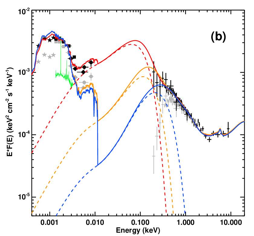
In the right panel of Figure 8, we use the same range of masses but aim instead to primarily fit the X-ray spectrum, and extrapolate the model to lower energies. The model with a (red curve) can fit the far UV (and variable optical) data, whereas the model for the and black hole masses under-predict the disc continuum by a factor of 10-50 as the peak of the disc spectrum shifts into the soft X-ray band, and its contribution to the UV and optical decreases.
6 Discussion
6.1 Black Hole Mass
Section 1 summarised previous mass estimates for RX1140 from RM (Rafter et al. 2011) and H. All previous black hole masses based on optical Spectra report RX1140 to be an IMBH with .
The X-ray variability power spectra also strongly support such a low mass, with no observed high frequency break on timescales longer than 500 s (see Figure. 2). This means that the total excess variance, , is high. We include our new data on the relation (Miniutti et al. 2009; Zhou et al. 2010; Ponti et al. 2012). Figure 9 shows the reverberation mapped subsample of objects from Ponti et al. (2012), where values were calculated from 40 ks light curves in the 2-10 keV bandpass. The best fit linear regression line is also shown. For RX1140, in Obs-1 and in Obs-2 (Obs-3 does not have sufficiently good data). These values correspond to . A mass lies outside the 2 region, but any mass within is consistent with the relation (see also Ludlam et al. 2015).
This highlights the inconsistency between the black hole mass derived from the SED models of , and all other mass determination methods which give . For a mass of , the SED models can either fit the optical/UV flux from the AGN, but then over-predict the X-rays, or they can fit the X-rays, but under-predict the optical/UV (Figure 8b). Given that the fraction of optical/UV flux from the AGN is constrained by the observed variability (Rafter et al. 2011), then this requires that the disc fit in Figure 8a) correctly describes the outer disc, with a derived . Clearly this is substantially super-Eddington, so there can be substantial energy loss via optically thick advection and/or winds from the inner disc. The fitted SED models, which assume that the disc is sub-Eddington so that neither of these processes is important (orange and blue curves in Figure fig-sed2a), then over-estimate the total luminosity.
The extent of the energy losses due to winds/advection can be estimated from the best fit SED model. The parameters of give ergs cm-2 s-1, which is around the Eddington limit for the most probable mass of . This is a supporting evidence for the proposal of Wang et al. (2014) that super-Eddington black holes have total luminosity which saturates around the Eddington limit.
However, RX1140 also has another unusual feature in that it exhibits strong optical variability, as seen in the RM campaign of Rafter et al. (2011). The majority of NLS1 show less optical variability than the broader line Seyferts (e.g. Ai et al. 2013, but see Kelly et al. 2013), which is somewhat surprising in view of their higher X-ray variability (e.g. Ponti et al. 2012). This unusually strong optical variability could indicate that some of the X-rays are reprocessed within a large scale wind. In which case the models above in Figure 8a, which require only disc emission to fit the optical, may be overestimating the mass accretion rate. Nonetheless there must be sufficient X-ray emission to power an additional optical component. The X-ray model fit based on shown in Figure 8b has an X-ray peak which has similar to the required far UV emission, so this model with would require that almost all the X-rays are reprocessed. A more likely reprocessing fraction of 10-50% then requires a higher Eddington ratio of . So perhaps the most plausible model is a combination of the two models in Figure 7a and Figure 7b, where the X-ray emission is partly suppressed by wind/advection losses and the optical emission is correspondingly enhanced by reprocessing in the wind.
We note that if winds and advection do play a significant role, it is curious that the X-ray spectrum and variability properties are not more noticeably different from other well studied NLS1 such as PG 1244+026, RE J1034+396 and RX J0136.9-3510 (e.g. Middleton et al. 2009; Jin et al. 2009; Jin et al. 2013). This then raises the possibility that these sources are likewise super-Eddington. PG 1244+026 has an SED which is acceptably well fit by a black hole accreting at about (Done et al. 2013). This SED has a distinct outer disc spectral shape in the optical/UV (e.g. Done et al. 2013), which constrains . Reducing the mass by a factor of 4 to i.e. removing the Marconi et al. (2008) radiation pressure correction to the H line width, then requires , which clearly means that this source could be very super-Eddington. However, this is probably an over-estimate as the well defined HF break in the power spectrum of this source (Jin et al. 2013) suggests at least a factor 5 higher mass than in RX1140, but this still gives . Advection and winds could also be significant in this source, which would invalidate the black hole spin determination described in Done et al. (2013).
If the majority of NLS1 are super-Eddington, but the typical Broad Line Seyfert 1’s have , then this implies a distinct bimodal (or a very long tail), mass accretion rate distribution. Also, such large energy losses due to advection/winds are probably not seen in the majority of Ultra-luminous X-ray sources (e.g. Sutton et al. 2015), although they may be present in the more extreme sources discussed by Gladstone, Done & Roberts (2009). The current data suggest that most of these sources represent moderately super-Eddington flows onto stellar mass black holes with masses around compared with those with seen in our Galaxy, due to their lower metallicity resulting in less mass loss from winds: Zampieri & Roberts (2009). Theoretical models predict quite high efficiency for these flows (Jiang, Stone & Davis 2014, but see also Sa̧dowski et al. 2015 who report lower efficiency). Clearly there remain are many aspects of super-Eddington accretion flows which are not yet understood.

7 Summary
In this paper we use new XMM-Newton data from one of the lowest mass AGN known to try to understand the nature of the soft X-ray excess, and how this fits in the context of its broad band SED. The mass from H (uncorrected for radiation pressure: Marconi et al. 2008), upper limit from reverberation mapping and fast X-ray variability are all consistent with a mass of . This, together with a steep 2-10 keV X-ray spectrum, and even steeper soft X-ray emission in this object make this a clear member of the ‘simple’ NLS1 class of AGN, where all objects with low black hole mass accreting at a high accretion rate.
We fit the time averaged X-ray data together with the covariance spectra of the fast variability to show that both low temperature Comptonisation and highly smeared, ionised reflection models can fit the data, but that both require an additional component at the lowest energies which we interpret as being from the inner disc. However, the RMS, lag and coherence spectra all point to a break in variability properties between the soft and hard X-ray bands, which is not consistent with the reflection models. Instead these support the low temperature Comptonisation model as this does not extend into the 2-10 keV band. All these properties are similar to other ‘simple’ NLS1 such as PG 1244+026 (Jin et al. 2013), RE J1934+396 (Middleton et al. 2009) and RX J0136.9-3510 (Jin et al. 2009).
However, putting the X-ray data into the context of the broadband SED reveals something quite new. The far UV and variable optical flux require an outer disc which has for an assumed mass of . This far over-predicts the soft X-ray emission for standard efficiency even assuming zero spin for the black hole. This strongly requires substantial energy loss via advection and/or winds unless the black hole mass is underestimated by a factor of 10, or the variable optical flux is not predominantly from the outer accretion disc (both of which seen extremely unlikely). If so, the other similar NLS1 are also likely to be similarly super-Eddington. This removes the requirement for low spin in these objects (Done et al. 2013), but also makes it highly unlikely that the geometry of these NLS1 are well represented by a flat disc, as used in reverberation studies.
Acknowledgements
This work is based on observations obtained with XMM-Newton, an ESA science mission with instruments and contributions directly funded by ESA Member States and NASA. This work makes use of data from SDSS, whose funding is provided by the Alfred P. Sloan Foundation, the Participating Institutions, the National Science Foundation, the U.S. Department of Energy, the National Aeronautics and Space Administration, the Japanese Monbukagakusho, the Max Planck Society, and the Higher Education Funding Council for England. We have made use of the ROSAT Data Archive of the Max-Planck-Institut für extraterrestrische Physik (MPE) at Garching, Germany.
References
- Ai et al. (2011) Ai Y. L., Yuan W., Zhou H. Y., Wang T. G., Zhang S. H., 2011, ApJ, 727, 31
- Ai et al. (2013) Ai Y. L., Yuan W., Zhou H., Wang T. G., Dong X. B., Wang J. G., Lu H. L., 2013, AJ, 145, 90
- Arnaud (1996) Arnaud K. A., 1996, ASPC, 101, 17
- Barth et al. (2004) Barth A. J., Ho L. C., Rutledge R. E., Sargent W. L. W., 2004, ApJ, 607, 90
- Baskin, Laor & Stern (2014) Baskin A., Laor A., Stern J., 2014, MNRAS, 438, 604
- Bentz et al. (2006) Bentz M. C., et al., 2006, ApJ, 651, 775
- Bentz et al. (2009a) Bentz M. C., Peterson B. M., Netzer H., Pogge R. W., Vestergaard M., 2009a, ApJ, 697, 160
- Bentz et al. (2009b) Bentz M. C., et al., 2009b, ApJ, 705, 199
- Bessell (1991) Bessell M. S., 1991, A&A, 242, L17
- Boroson (2002) Boroson T. A., 2002, ApJ, 565, 78
- Boroson & Green (1992) Boroson T. A., Green R. F., 1992, ApJS, 80, 109
- Cardelli et al. (1989) Cardelli J. A., Clayton G. C., Mathis J. S., 1989, ApJ, 345, 245
- Davis & Laor (2011) Davis S. W., Laor A., 2011, ApJ, 728, 98
- Denney et al. (2006) Denney K. D., et al., 2006, ApJ, 653, 152
- Denney et al. (2010) Denney K. D., et al., 2010, ApJ, 721, 715
- Done et al. (2012) Done C., Davis S. W., Jin C., Blaes O., Ward, M., 2012, MNRAS, 420, 1848 (D12)
- Done et al. (2013) Done C., Jin C., Middleton M., Ward M., 2013, MNRAS, 434, 1955
- Dong et al. (2007) Dong X., et al., 2007, ApJ, 657, 700
- Du et al. (2014) Du P., et al., 2014, ApJ, 782, 45
- Edelson et al. (2002) Edelson R., Turner T. J., Pounds K., Vaughan S., Markowitz A., Marshall H., Dobbie P., Warwick R., 2002, ApJ, 568, 610
- Elvis et al. (1994) Elvis M., et al., 1994, ApJS, 95, 1
- Fabian, Kara & Parker (2014) Fabian A. C., Kara E., Parker M. L., 2014, Suzaku-MAXI 2014: Expanding the Frontiers of the X-ray Universe, 279
- Fabian & Miniutti (2005) Fabian A. C., Miniutti, G., 2005, arXiv:astro-ph/0507409
- Fabian et al. (2009) Fabian A. C., et al., 2009, Nature, 459, 540
- Fabian et al. (2013) Fabian A. C., et al., 2013, MNRAS, 429, 2917
- Filippenko & Ho (2003) Felippenko A. V., Ho L. C., 2003, ApJ, 588L, 13
- Gardner & Done (2015) Gardner E., Done C., 2015a, MNRAS, 448, 2245
- Gierliński & Done (2004) Gierliński M., Done C., 2004, MNRAS, 349, L7
- Gladstone et al. (2009) Gladstone J. C., Roberts T. P., Done C., 2009, MNRAS, 397, 1836
- Gierliński & Done (2006) Gierliński M., Done C., 2006, MNRAS, 371, L16
- Greene & Ho (2004) Greene J. E., Ho L. C., 2004, ApJ, 610, 722
- Greene & Ho (2007) Greene J. E., Ho L. C., 2007, ApJ, 670, 92
- Greene, Ho & Barth (2008) Greene J. E., Ho L. C., Barth A. J., 2008, ApJ, 688, 159
- Hua & Titarchuk (1995) Hua X.-M., Titarchuk L., 1995, ApJ, 449, 188
- Jiang et al. (2014) Jiang Y. F., Stone J. M., Davis S. W., 2014, ApJ, 796, 106
- Jin et al. (2013) Jin C., Done C., Middleton M., Ward M., 2013, MNRAS, 436, 3173
- Jin et al. (2009) Jin C., Done C., Ward M., Gierliński M., Mullaney J., 2009, MNRAS, 398, L16
- Jin, Ward & Done (2012b) Jin C., Ward M., Done C., 2012b, MNRAS, 422, 3268 (J12b)
- Jin, Ward & Done (2012c) Jin C., Ward M., Done C., 2012c, MNRAS, 425, 907 (J12c)
- Jin et al. (2012a) Jin C., Ward M., Done C., Gelbord J., 2012a, MNRAS, 420, 1825 (J12a)
- Kalberla et al. (2005) Kalberla P. M. W., Burton W. B., Hartmann D., Arnal E. M., Bajaja E., Morras R., Pöppel W. G. L., 2005, A&A, 440, 775
- Kelly et al. (2013) Kelly B. C., Treu T., Malkan M., Pancoast A., Woo J. H., 2013, ApJ, 779, 187
- Kaspi et al. (2000) Kaspi S., Smith P. S., Netzer H., Maoz D., Jannuzi B. T., Giveon U., 2000, ApJ, 533, 631
- Kunth, Sargent & Bothun (1987) Kunth D., Sargent W. L. W., Bothun G. D., 1987, AJ, 93, 29
- Laor (1991) Laor A., 1991, ApJ, 376, 90
- Laor et al. (1997) Laor A., Fiore F., Elvis M., Wilkes B. J., McDowell J. C., 1997, ApJ, 477, 93
- Leighly (1999) Leighly K. M., 1999, ApJS, 125, 317
- Ludlam et al. (2015) Ludlam R. M., Cackett E. M., Gültekin K., Fabian A. C., Gallo L., Miniutti G., 2015, MNRAS, 447, 2112
- Magdziarz et al. (1998) Magdziarz P., Blaes O. M., Zdziarski A. A., Johnson W. N., Smith D. A., 1998, MNRAS, 301, 179
- Makishima et al. (1986) Makishima K., Maejima Y., Mitsuda K., Bradt H. V., Remillard R. A., Tuohy I. R., Hoshi R., Nakagawa M., 1986, ApJ, 308, 635
- Marconi et al. (2008) Marconi A., Axon D. J., Maiolino R., Nagao T., Pastorini G., Pietrini P., Robinson A., Torricelli G., 2008, ApJ, 678, 693
- Marconi et al. (2009) Marconi A., Axon D. J., Maiolino R., Nagao T., Pietrini P., Risaliti G., Robinson A., Torricelli G., 2009, ApJ, 698, L103
- Markowitz et al. (2003) Markowitz A., Edelson R., Vaughan S., 2003, ApJ, 598, 935
- Matt et al. (2014) Matt G., et al., 2014, MNRAS, 439, 3016
- McHardy et al. (2004) McHardy I. M., Papadakis I. E., Uttley P., Page M. J., Mason K. O., 2004, MNRAS, 348, 783
- Middleton et al. (2009) Middleton M., Done C., Ward M., Gierliński M., Schurch N., 2009, MNRAS, 394,250
- Miniutti et al. (2009) Miniutti G., Ponti G., Greene, J. E., Ho L. C., Fabian A. C., Iwasawa K., 2009, MNRAS, 394, 443
- Mitsuda et al. (1984) Mitsuda K., et al., 1984, PASJ, 36, 741
- Morrison & McCammon (1983) Morrison R., McCammon D., 1983, ApJ, 270, 119
- Nandra et al. (2007) Nandra K., O’Neill P. M., George I. M., Reeves, J. N., 2007, MNRAS, 382, 194
- Nowak et al. (1999) Nowak M. A., Wilms J., Vaughan B. A., Dove J. B., Begelman M. C., 1999, ApJ, 515, 726
- Osterbrock & Pogge (1985) Osterbrock D. E., Pogge R. W., 1985, ApJ, 297, 166
- Rafter et al. (2011) Rafter S. E., Kaspi S., Behar E., Kollatschny W., Zetzl M., 2011, ApJ, 741, 66
- Peterson (1997) Peterson B. M., 1997, An introduction to active galactic nuclei, Publisher: Cambridge, New York Cambridge University Press, 1997 Physical description xvi, 238 p. ISBN 0521473489
- Peterson et al. (2004) Peterson B. M., et al., 2004, ApJ, 613, 682
- Peterson et al. (2005) Peterson B. M., et al., 2005, ApJ, 632, 799
- Polletta et al. (2007) Polletta M., et al., 2007, ApJ, 663, 81
- Ponti et al. (2012) Ponti G., Papadakis I., Bianchi S., Guainazzi M., Matt G., Uttley P., Bonilla N. F., 2012, A&A, 542, A83
- Sa̧dowski et al. (2015) Sa̧dowski A., Narayan R., Tchekhovskoy A., Abarca D., Zhu Y., McKinney J. C., 2015, MNRAS, 447, 49
- Schurch & Done (2007) Schurch N. J., Done C., 2007, MNRAS, 381, 1413
- Sutton et al. (2015) Sutton A. D, Roberts T. P., Gladstone J. C., Walton D. J., 2015, arXiv:1503.01711
- Titarchuk (1994) Titarchuk L., 1994, ApJ, 434, 570
- Titarchuk & Lyubarskij (1995) Titarchuk L., Lyubarskij Y., 1995, ApJ, 450, 876
- Uttley et al. (2014) Uttley P., Cackett E. M., Fabian A. C., Kara E., Wilkins D. R., 2014, A&ARv, 22, 72
- Vaughan et al. (2003) Vaughan S., Edelson R., Warwick R. S., Uttley P., 2003, MNRAS, 345, 1271
- Wang et al. (2014) Wang J. M., et al., 2014, ApJ, 793, 108
- Wilkinson & Uttley (2009) Wilkinson T., Uttley P., 2009, MNRAS, 397, 666
- Zampieri & Roberts (2009) Zampieri L., Roberts, T. P., 2009, MNRAS, 400, 677
- Zdziarski et al. (1996) Zdziarski A. A., Johnson W. N., Magdziarz P., 1996, MNRAS, 283, 193
- Zhang & Wang (2006) Zhang E. P., Wang J. M., 2006, ApJ, 653, 137
- Zhou et al. (2010) Zhou X. L., Zhang S. N., Wang D. X., Zhu L., 2010, ApJ, 710, 16
- Zoghbi et al. (2010) Zoghbi A., Fabian A. C., Uttley P., Miniutti G., Gallo L. C., Reynolds C. S., Miller J. M., Ponti G., 2010, MNRAS, 401, 2419
- Życki et al. (1999) Życki P. T., Done C., Smith D. A., 1999, MNRAS, 309, 561