On Locally Dyadic Stationary Processes
First Revision: April 2016
Second Revision: September 2016
Abstract
We introduce the concept of local dyadic stationarity, to account for non-stationary time series, within the framework of Walsh-Fourier analysis. We define and study the time varying dyadic ARMA models (tvDARMA). It is proven that the general tvDARMA process can be approximated locally by either a tvDMA and a tvDAR process.
Keywords: dyadic stationarity, local stationarity, spectral density, stationarity, Walsh functions, Walsh-Fourier analysis.
1 Introduction
The concept of stationarity is crucial in the statistical theory of time series analysis, especially for the development of asymptotic theory. However, the assumption of stationarity is often not realistic in applications. For example, a time series can display significant changes through time and therefore stationarity is a questionable assumption. One of the most important consequences, is that attempts to develop asymptotic results are, generally speaking, groundless, since future information of the process does not necessarily contain any information regarding the present of the process. In addition, there is no natural generalization of stationarity to non-stationarity, since non-stationary processes might exhibit trend or/and periodicity and other types of non-standard behaviour.
Priestley (1965) considered non-stationary processes whose characteristics are changing slowly over time and developed the theory of evolutionary spectra (see Priestley (1981); Priestley (1988)). However, such an approach makes it difficult to obtain asymptotic results, which are needed for developing estimation theory. In order to apply standard asymptotic theory for non-stationary processes, Dahlhaus, in a series of contributions, introduced an appropriate theoretical framework, based on the concept of local stationarity (see, for example, Dahlhaus (1996b); Dahlhaus (1997); Dahlhaus (2000)). The definition of local stationarity is based on the existence of a time varying spectral representation (Dahlhaus (1996b)). Dahlhaus (2012) gives an excellent and detailed overview of the theory of locally stationary processes. A comparison between the methodology developed by Dahlhaus and Priestley is discussed in Dahlhaus (1996a). Some other works related to locally stationary time series include the works by Granger and Hatanaka (1964), Tjøstheim (1976), Martin (1981), Melard and Schutter (1989), Neumann and Von Sachs (1997), Nason et al. (2000), Ombao et al. (2002), Sakiyama and Taniguchi (2004) and Davis et al. (2006), among others.
The main goal of this contribution is to utilize the idea of local stationarity, in the sense of the above mentioned papers, for studying the spectral behaviour of time series, based on the system of Walsh functions. These functions led to the development of Walsh-Fourier (square wave) analysis, just like the sinusoidal functions led to Fourier (trigonometric) analysis. The motivation behind Walsh-Fourier analysis was the need to approximate stationary time series, which display square waveforms with abrupt switches (e.g. in communications and engineering), see Stankovic̀ et al. (2005) for instance. We introduce the concept of local stationarity but based on the orthogonal system of Walsh functions to account for such phenomena that exhibit, in addition, non-stationary behaviour. We study important general classes of time series, similar in concept with the time varying ARMA (tvARMA) process- see Dahlhaus (2012). We anticipate that our theory and methods will be applicable to non-stationary data observed in diverse applications like pattern recognition for binary images, linear system theory and other (see Stankovic̀ et al. (2005), for more).
The Walsh functions were introduced by Walsh (1923). They take only two values, and , and have similar properties with the trigonometric functions (although they are not periodic). The introduction of Walsh functions has been followed by a series of papers, related to their mathematical properties and generalizations (Fine (1949)), which provided the theoretical framework for various applications, see e.g. Beauchamp (1984), Stoffer (1991) and Abbasi et al. (2012), among others. Stoffer (1991) gives an excellent account of the history of Walsh functions and a comparison between Walsh and Fourier analysis.
The statistical analysis of stationary time series via Walsh functions has been based on real and dyadic time. The dyadic time is based on the concept of dyadic addition (see Subsection 2.1). For time points , the real time sum is now replaced by the dyadic sum Morettin (1981) reviewed work on Walsh spectral analysis in both time scales. Walsh-Fourier analysis of real time stationary processes has been studied by Kohn (1980a); Kohn (1980b), Morettin (1983) and Stoffer (1985); Stoffer (1987); Stoffer (1990), among others. The dyadic time stationarity is defined in respect to the real time stationarity as in Subsection 2.2 (see also Nagai (1977)). Further references related to the Walsh-Fourier analysis of dyadic stationary processes are Morettin (1974); Morettin (1978); Morettin (1981), Nagai (1980), Nagai and Taniguchi (1987) and Taniguchi et al. (1989). In particular, Morettin (1974); Morettin (1978) studied the finite Walsh transform, considered the Walsh periodogram as an estimator of the Walsh spectrum and studied its theoretical properties. Nagai (1977) proved that a dyadic stationary process has always unique spectral representation in terms of the system of Walsh functions and studied the dyadic linear process (see also Morettin (1974)). Nagai (1980) also studied dyadic autoregressive and moving average processes and their relation.
In this article, we introduce the concept of local dyadic stationarity and discuss the advantages and the perspectives of such consideration in the framework of Walsh functions. In Section of this article, we recall some definitions and review some fundamental results for dyadic stationary processes. In Section , we introduce the concept of local dyadic stationarity and study the time varying dyadic moving average process. In Section , we define the general class of time varying dyadic autoregressive moving average processes and show that they exhibit locally dyadic stationarity. The article concludes with several remarks concerning further research in this topic.
2 Preliminaries
2.1 Dyadic addition
We recall the definition of dyadic addition and of a dyadic process following Kohn (1980a). Consider and to be non-negative integers that have the following dyadic expansions
Then, the dyadic sum is defined as
Consider now and to be real numbers that belong to the interval We write
In general, each of the above representations is not unique. We follow the convention that if, e.g. can be written both through a finite or an infinite order representation, then choose the representation where . With this convention, the dyadic sum is defined as
Recall that the - Rademacher function is Then the system of Walsh functions, is defined as follows. If set For , let where . Then
We mention briefly some characteristic properties of the Walsh functions.
(i) The system of Walsh functions is orthonormal in , that is
and constitutes a complete set. If is a square integrable function, then it can be expanded in a Walsh-Fourier series, i.e.
with
(ii) and
The above properties of Walsh functions motivate the study of stationary time series in terms of this basis. It is well known that a second order stationary process is represented as
with an orthogonal-increment process such that
where is the Dirac function periodically extended to with period and is the spectral distribution function (see Brillinger (1974), for instance).
The Walsh functions can be used instead to represent under the concept of dyadic stationarity. There are differences though between real and dyadic stationary processes; see Morettin (1981) for further discussion. The concept of dyadic stationarity is explained briefly next.
2.2 Dyadic stationarity
We call a stochastic process dyadic stationary if it has constant mean, finite second moment and its covariance function
is invariant under dyadic addition, i.e. it depends only on Hence, we write for notational convenience In the following assume that We recall some important results about dyadic stationary processes.
A dyadic stationary process has a dyadic spectral representation given by (Morettin (1974, p. 193))
where is a real random process with orthogonal increments, such that
where is the Dirac function periodically extended to with period 1. The function , defined on , is a unique distribution function, which is called the dyadic spectral distribution of the process In addition
If is absolutely continuous, then where is called the dyadic spectral density of
Example 1.
A simple example of a dyadic stationary process is a sequence of independent random variables with . It is straightforward to show that its covariance function is
Since the sequence is dyadic stationary, it has a dyadic spectral representation of the form
with
This example illustrates the analogy of dyadic and real time stationary processes. Indeed, it is well known that a white noise real time process possesses a flat spectrum; the same is true under dyadic stationarity.
A stochastic process is a linear dyadic process if it can be represented as (Morettin (1974))
| (1) |
where is the sequence of i.i.d. variables, as in Example 1, and are real numbers, which satisfy This definition is similar in spirit to the definition of the general linear process Priestley (1981, p.415).
It can be shown that a linear dyadic process of the form (1) is dyadic stationary, because
| (2) |
In addition, it has an absolutely continuous dyadic spectral distribution function and its dyadic spectral density function has the form
| (3) |
where In this case, note that , for . Again, we note the analogy between real time and dyadic stationarity; the above formula is identical to the formula obtained in the real time linear process model (Priestley (1981)). Furthermore, if and in (1), then is said to be a dyadic moving average process of order , abbreviated as DMA. In general, the process defined by (1) is called a DMA process.
3 Local Dyadic Stationarity
Consider now (3), and suppose, for example, that the function depends upon time, i.e. it has the form where denotes the sample size. is now reexpressed as a triangular array We rescale from the axis of the first non negative integers () to the unit interval . The reason for this rescaling will be clear later on. The rescaled form of is denoted by . We give a general definition regarding local dyadic stationarity for a process , in the spirit of Dahlhaus (e.g Dahlhaus (1996b); Dahlhaus (1997)).
Definition 1.
A sequence of stochastic processes is called locally dyadic stationary with transfer function and trend function where and are deterministic functions, if there exists a representation
| (4) |
where the following hold:
(i) is a real-valued stochastic process on and
where denotes the - order cumulant, are bounded for all and denotes the
Dirac delta function periodically extended to with period 1.
(ii) There exists a constant and a function such that
| (5) |
The functions and are assumed to be continuous with respect to .
The above definition is analogous to the definition given by Dahlhaus (1996b). The first condition states that the has moments of order ; the functions are the - polyspectrum of following Brillinger (1965). The second assumption requires that the transfer function is approximated locally by a function which is the transfer function of a dyadic stationary process. Note that the continuity of and in is required for the process to exhibit locally dyadic stationary behaviour. Furthermore, without loss of generality, we assume that because the transfer function can be always rescaled such that the process is white noise. Indeed, the boundedness assumption of implies again (5) for the rescaled transfer function.
Example 2.
Suppose is a dyadic stationary process with dyadic spectral representation
where Define by
where are continuous functions defined on . Then
where and the assumptions and are satisfied. Hence is locally a dyadic stationary process.
Consider now the process
| (6) |
where is an i.i.d. sequence and is a time-dependent process of real numbers such that . We call this process a time varying dyadic moving average process of infinite order (tvDMA). If we set in (6) and then we call a time varying dyadic moving average process of order (tvDMA). We rescale now the parameter curves to the unit interval , assuming that there exist functions that satisfy We further assume that satisfy some regularity conditions (see Remark 2). The reasons for the rescaling are described in detail, e.g. in Dahlhaus (2012, Sec.2). Briefly, suppose that we choose to be polynomials of . Then, as , as well, which violates the condition In addition, rescaling enables us to impose smoothing conditions through the continuity of the functions ensuring that the process exhibits locally dyadic stationary behaviour. Indeed, the number of observations within the neighbourhood of a fixed point increases as enabling to develop and apply locally for asymptotic results for dyadic stationary processes. Suppose that the process defined by (6) is written as
We assume that for and for and that the functions satisfy some standard smoothness conditions; see Dahlhaus (1997). Consider now a fixed point and its neighborhood If the length of this segment is sufficiently small, the process can be approximated by the process which is defined as
where are constants, with indicating their dependence from the fixed point (see also Dahlhaus (2012)). is dyadic stationary. Indeed, we can write
| (7) |
where
From equations (2) and (3), has covariance function
and a unique dyadic spectral density function given by
where indicates the dependence from a fixed point.
We can show that for it holds , see Corollary 1. Therefore, we can say that has locally the same covariance and dyadic spectral density function as and therefore exhibits locally dyadic stationary behaviour. Note that the tvDMA process in (6) is locally dyadic stationary due to Definition 1, since it has a time varying spectral representation as in (4). Indeed, we have
where is the time varying transfer function. We show in Theorem 1 that, in general, a locally dyadic stationary process is approximated by a dyadic stationary process within a given interval.
Theorem 1.
Suppose that is a sequence of stochastic processes which satisfy a representation of the form (4) where is the time varying transfer function (set ). Suppose that is a dyadic stationary process with
| (8) |
where depends on the fixed point . Then within an interval and under the assumptions of Definition 1 it holds that
Proof.
| (9) | |||||
since In addition
| (10) | |||||
from (5) in assumption (ii) of Definition 1. However, the same assumption states that is continuous. Therefore, since and for any we can choose to be such that (10) becomes
| (11) |
for some positive constant Finally, from (9) and (11), we obtain that
and hence we have the desired result. ∎
 |
 |
Corollary 1.
Remark 1.
Theorem 1 implies that a locally dyadic stationary process could be approximated by dyadic stationary processes within different intervals in (that may overlap). Thus its behaviour could be described via the behaviour of those dyadic stationary processes.
Remark 2.
Equation (5) implies a similar assumption for the and the above discussion still holds.
Example 3.
Consider, for example, the infinite time varying MA (tvMA) representation in the real time. Then its time varying spectral density function is given by
Respectively, the time varying dyadic spectral density function of the tvDMA is given by
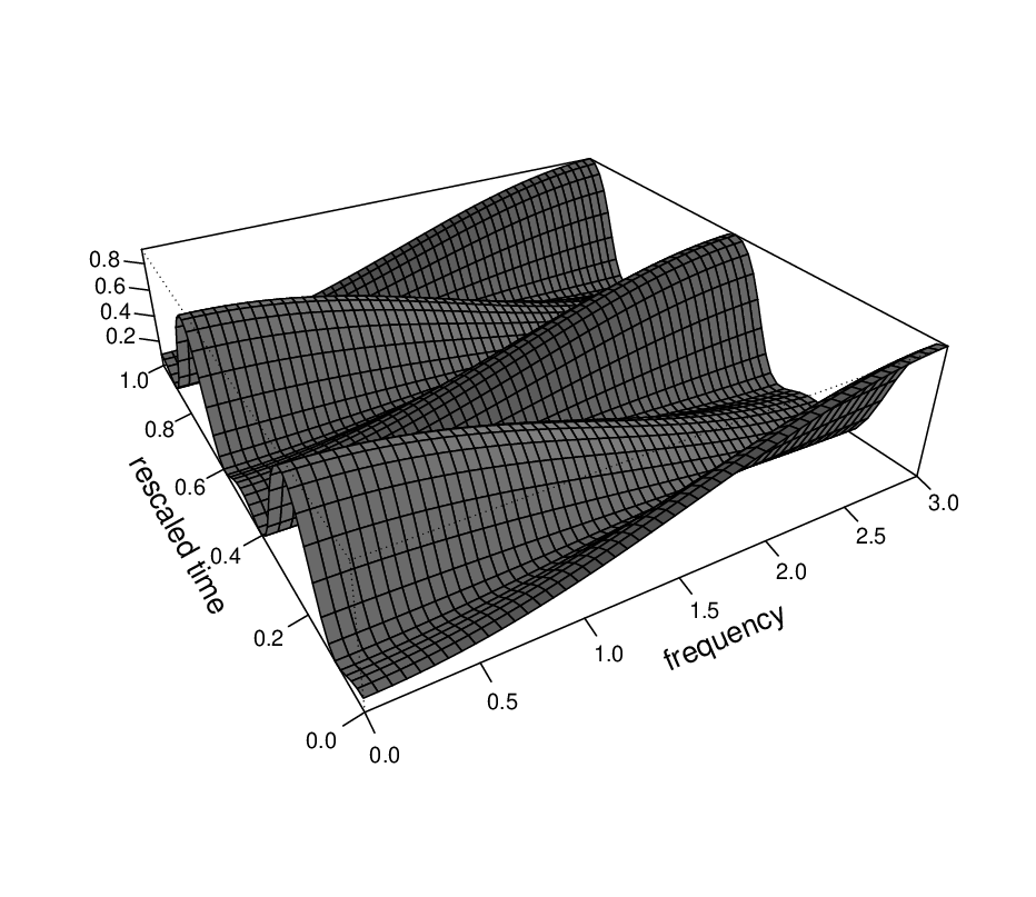
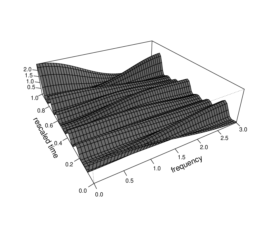
We compare the behaviour of functions and for the same order of the respective processes and for the same representation of the time varying coefficients (set ). Figure 1 shows the spectral density function of a tvMA and tvDMA processes. We set and Figure 2 shows the spectral density function of a tvMA and tvDMA processes. In this case we set and Both figures reveal the differences between real and dyadic stationarity. The square waveform of Walsh functions allows a more oscillatory behaviour of the dyadic spectral density function.
 |
 |
4 tvDARMA processes
It is well known that autoregressive, moving average, and ARMA models can be regarded as special cases of the general linear process. Nagai (1980) shows that a dyadic autoregressive process of finite order is always inverted into a dyadic moving average process of finite order, and vice versa. We obtain similar results, but within a time varying framework. We define the time varying, dyadic, autoregressive, moving average (tvDARMA) process as follows.
Definition 2.
A stochastic process is called tvDARMA if it is locally dyadic stationary and can be represented by
| (12) |
where with the sequences of parameters are real numbers with at least two non-zero parameters for and In addition, is an i.i.d. sequence with and .
Assume that If we set in (12), , then the tvDMA process arises as in (6), but for a finite order . In case we set in (12) , then (12) becomes
| (13) |
We call in (13) a time varying, dyadic, autoregressive process of order (tvDAR). We show that a tvDAR process, and even more generally, a tvDARMA process, can be approximated by a tvDMA process. Following Nagai and Taniguchi (1987), who study multivariate dyadic stationary processes, set
| (14) |
where and are real numbers. Denote by the matrix, which is given by
Lemma 1.
The following equation holds
where Therefore the function if and only if
Lemma 2.
Assume that in (14). Then there exists a function , which is defined by
and satisfies The coefficients are uniquely determined by
Define to be the matrix
The following theorem states that a tvDARMA process can be approximated locally by a tvDMA and a tvDAR process.
Theorem 2.
Suppose that is a tvDARMA as in (12). Set .
Then the following hold
(i) If then can be approximated locally by a tvDMA process.
(ii) If then can be approximated locally by a tvDAR process.
Corollary 2.
Suppose that is a tvDAR as in (13). If can be approximated locally by a tvDMA process.
Proofs of these results are given in the appendix.
5 Conclusions
We anticipate that the above results will be useful for future work in the field of applications. In this direction, the concepts of Walsh spectrum and Walsh transform will be studied. The Walsh spectrum for a real-valued dyadic stationary process is defined by
| (15) |
where the covariance function satisfies (see e.g. Morettin (1974); Morettin (1978); Morettin (1981)). Inverting (15), the covariance is given by
The finite Walsh transform is given by
To estimate the Walsh spectrum, Morettin (1981) defined the Walsh periodogram, by
and showed that is asymptotically an unbiased, but inconsistent, estimator of He also considered the smooth Walsh periodogram and other classes of estimates. Dyadic stationarity is necessary to estimate the time-varying Walsh spectrum. Therefore, in the case of local dyadic stationarity, it would be reasonable to divide the rescaled interval into subintervals and estimate the Walsh spectrum within each subinterval, where local dyadic stationarity is satisfied. The number of the observations within each subinterval increases as tends to infinity and the above asymptotical results still hold. A similar method is applied by Dahlhaus and Giraitis (1998) for real-time stationary processes.
Kohn (1980a); Kohn (1980b) studied the system of Walsh functions for real time stationary processes. He defined the - logical autocovariance, , and the corresponding Walsh-Fourier spectral density function . This notation replaces the previous notation used for and above. He considered the finite Walsh-Fourier transform and studied its asymptotic properties. A class of estimators for was obtained, the average Walsh periodogram being a member of this class. The concept of local stationarity could also be applied in the real time setting and we conjecture that similar results could be obtained also in this case.
Acknowledgements
We cordially thank Prof. I. Nikiforov and four anonymous reviewers for several constructive comments that improved considerably an earlier version of the manuscript.
Appendix
Proof of Lemma 1
Recall that . The Walsh-ordered Hadamard matrix is a matrix with elements of the form , see also Stoffer (1991). Then the following relations hold:
For the second argument of Lemma 1, note that and every Walsh function remains invariant for and equal to . Therefore
Proof of Lemma 2
Proof of Theorem 2
Since is locally dyadic stationary it has a Walsh spectral representation
while is dyadic stationary and represented by
Then the LHS and RHS of equation (12) can be written as
| LHS | (A-34) |
and
| RHS |
Set
| (A-35) |
Then
| (A-36) | |||||
Consider the interval . Then, , we can assume that is large enough, such that From the continuity of the function and assumption (5) we have that
| (A-37) | |||||
since and , with and real constants.
Proof of Corollary 2
References
- Abbasi et al. (2012) Abbasi, S. A., A. Alamoud, et al. (2012). FPGA based Walsh and inverse Walsh transforms for signal processing. Elektronika ir Elektrotechnika 18, 3–8.
- Beauchamp (1984) Beauchamp, K. G. (1984). Walsh functions and their applications. Academic Press.
- Brillinger (1965) Brillinger, D. R. (1965). An introduction to polyspectra. The Annals of mathematical statistics, 1351–1374.
- Brillinger (1974) Brillinger, D. R. (1974). Fourier analysis of stationary processes. Proc. IEEE 62, 1628–1643.
- Dahlhaus (1996a) Dahlhaus, R. (1996a). Asymptotic statistical inference for nonstationary processes with evolutionary spectra. In Athens conference on applied probability and time series analysis, pp. 145–159. Springer.
- Dahlhaus (1996b) Dahlhaus, R. (1996b). On the Kullback-Leibler information divergence of locally stationary processes. Stochastic Processes and their Applications 62, 139–168.
- Dahlhaus (1997) Dahlhaus, R. (1997). Fitting time series models to nonstationary processes. The Annals of Statistics 25, 1–37.
- Dahlhaus (2000) Dahlhaus, R. (2000). A likelihood approximation for locally stationary processes. Annals of Statistics 28, 1762–1794.
- Dahlhaus (2012) Dahlhaus, R. (2012). Locally stationary processes. In T. S. Rao, S. S. Rao, and C. R. Rao (Eds.), Handbook of Statistics: Time Series Analysis–Methods and Applications, Volume 30, pp. 351–408. Amsterdam: Elsevier B. V.
- Dahlhaus and Giraitis (1998) Dahlhaus, R. and L. Giraitis (1998). On the optimal segment length for parameter estimates for locally stationary time series. Journal of Time Series Analysis 19, 629–655.
- Davis et al. (2006) Davis, R. A., T. C. M. Lee, and G. A. Rodriguez-Yam (2006). Structural break estimation for nonstationary time series models. Journal of the American Statistical Association 101, 223–239.
- Fine (1949) Fine, N. J. (1949). On the Walsh functions. Transactions of the American Mathematical Society 65, 372–414.
- Granger and Hatanaka (1964) Granger, C. W. J. and M. Hatanaka (1964). Spectral analysis of economic time series. Princeton: Univ. Press.
- Kohn (1980a) Kohn, R. (1980a). On the spectral decomposition of stationary time series using Walsh functions. I. Advances in Applied Probability, 183–199.
- Kohn (1980b) Kohn, R. (1980b). On the spectral decomposition of stationary time series using Walsh functions. II. Advances in Applied Probability, 462–474.
- Martin (1981) Martin, W. (1981). Line tracking in nonstationary processes. Signal Processing 3, 147–155.
- Melard and Schutter (1989) Melard, G. and A. H.-d. Schutter (1989). Contributions to evolutionary spectral theory. Journal of Time Series Analysis 10, 41–63.
- Morettin (1974) Morettin, P. A. (1974). Walsh-function analysis of a certain class of time series. Stochastic processes and their applications 2, 183–193.
- Morettin (1978) Morettin, P. A. (1978). Estimation of the spectrum and of the covariance function of a dyadic-stationary series. Bulletin of the Brazilian Mathematical Society 9, 83–88.
- Morettin (1981) Morettin, P. A. (1981). Walsh spectral analysis. SIAM Review 23, 279–291.
- Morettin (1983) Morettin, P. A. (1983). A note on a central limit theorem for stationary processes. Journal of Time Series Analysis 4, 49–52.
- Nagai (1977) Nagai, T. (1977). Dyadic stationary processes and their spectral representations. Bulletin of Mathematical Statistics 17, 65–73.
- Nagai (1980) Nagai, T. (1980). On finite parametric linear models of dyadic stationary processes. Bulletin of Mathematical Statistics 19, 45–53.
- Nagai and Taniguchi (1987) Nagai, T. and M. Taniguchi (1987). Walsh spectral analysis of multiple dyadic stationary processes and its applications. Stochastic Processes and their Applications 24, 19–30.
- Nason et al. (2000) Nason, G. P., R. Von Sachs, and G. Kroisandt (2000). Wavelet processes and adaptive estimation of the evolutionary wavelet spectrum. Journal of the Royal Statistical Society: Series B (Statistical Methodology) 62, 271–292.
- Neumann and Von Sachs (1997) Neumann, M. H. and R. Von Sachs (1997). Wavelet thresholding in anisotropic function classes and application to adaptive estimation of evolutionary spectra. The Annals of Statistics 25, 38–76.
- Ombao et al. (2002) Ombao, H., J. Raz, R. von Sachs, and W. Guo (2002). The slex model of a non-stationary random process. Annals of the Institute of Statistical Mathematics 54(1), 171–200.
- Priestley (1965) Priestley, M. B. (1965). Evolutionary spectra and non-stationary processes. Journal of the Royal Statistical Society. Series B (Methodological) 27, 204–237.
- Priestley (1981) Priestley, M. B. (1981). Spectral analysis and time series. Academic Press, London.
- Priestley (1988) Priestley, M. B. (1988). Non-linear and non-stationary time series analysis. Academic Press, London.
- Sakiyama and Taniguchi (2004) Sakiyama, K. and M. Taniguchi (2004). Discriminant analysis for locally stationary processes. Journal of Multivariate Analysis 90, 282–300.
- Stankovic̀ et al. (2005) Stankovic̀, R. S., C. Moraga, and J. Astola (2005). Fourier Analysis on Finite Groups with Applications in Signal Processing and System Design. Hoboken, NJ: Wiley-IEEE.
- Stoffer (1985) Stoffer, D. S. (1985). Central limit theorems for finiteWalsh-Fourier transforms of weakly stationary time series. Journal of Time Series Analysis 6, 261–267.
- Stoffer (1987) Stoffer, D. S. (1987). Walsh-Fourier analysis of discrete-valued time series. Journal of Time Series Analysis 8, 449–467.
- Stoffer (1990) Stoffer, D. S. (1990). Multivariate Walsh-Fourier analysis. Journal of Time Series Analysis 11, 57–73.
- Stoffer (1991) Stoffer, D. S. (1991). Walsh-Fourier analysis and its statistical applications. Journal of the American Statistical Association 86, 461–479.
- Taniguchi et al. (1989) Taniguchi, M., L. Zhao, P. Krishnaiah, and Z. Bai (1989). Statistical analysis of dyadic stationary processes. Annals of the Institute of Statistical Mathematics 41, 205–225.
- Tjøstheim (1976) Tjøstheim, D. (1976). Spectral generating operators for non-stationary processes. Advances in Applied Probability 8, 831–846.
- Walsh (1923) Walsh, J. (1923). A closed set of normal orthogonal functions. American Journal of Mathematics 45, 5–24.