Transitions in the Stock Markets of the US, UK, and Germany

Matthias Raddant Affiliation: Institute for the World Economy
Kiellinie 66, Kiel 24105, Germany,
and
Department of Economics, Kiel University
Olshausenstr. 40, 24118 Kiel, Germany,
matthias.raddant@ifw-kiel.de, Friedrich Wagner Affiliation: Institute of Theoretical Physics, Kiel University
Leibnizstr. 19, Kiel 24098, Germany, wagner@theo-physik.uni-kiel.de

Abstract

In an analysis of the US, the UK, and the German stock market we find a change in the behavior based on the stock’s beta values. Before 2006 risky trades were concentrated on stocks in the IT and technology sector. Afterwards risky trading takes place for stocks from the financial sector. We show that an agent-based model can reproduce these changes. We further show that the initial impulse for the transition might stem from the increase of high frequency trading at that time.

An earlier version of this paper is available as Kiel Working Paper No. 1979.

Keywords:

stock price correlations ; financial risk ; CAPM

I Introduction

In this paper we analyze transitions in the structure of the US, the UK, and the German stock market. In particular we observe a phase of dominance of IT oriented stocks followed by a transition period that leads to a dominance of the financial sector.

The analysis of the differences in the returns of stocks have long been dominated by the discussions around different versions of a CAPM model [18, 26]. The original version of the CAPM is in fact a one factor model, which postulates that the returns $r_{i}$ of the stocks should be governed by the market return $r_{M}$ and only differ by an idiosyncratic component $\beta_{i}$ for each stock $i$ , such that

\displaystyle r_{i}(t)=\beta_{i}r_{M}(t)+\epsilon_{i}(t).

(1)

Hence, stocks differ by the amount of volatility with respect to the market, and economic rational necessitates that higher stock volatility is compensated by higher absolute returns (additionally eq. may incorporate the risk free interest rate). Empirical tests of this model had rather mixed results and have let to two conclusions: More factors are needed to explain the variation of stock returns. The widely used Fama and French [12] model for example is a three-factor model that incorporates firm size and book-to-market ratio. The second conclusion was that beta values are not constant but time-varying, see [7]. The reasons for the variability of the betas are manifold. They could change due to microeconomic factors, the business environment, macroeconomic factors, or due to changes of expectations, see, e.g., [5, 1, 13]. Also models that assume a first-order auto-regressive process have been suggested, see [6].

Our approach to identify different states of a stock market consists in an analysis of a covariance matrix, similar to [22], and of the transaction volumes, like in [24]. The properties of the covariance matrix of asset returns depend on the time horizon $T$ in which they are determined. For short $T$ in the order of months they are rather volatile, and partly mirror economic and political changes [16, 15]. [4] for example argue that correlations increase in times of crisis, which has profound implication for portfolio choice and hedging of risks.

For large $T$ in the order of several years, a principal component analysis [17, 23, 19] of the correlation matrix is possible. The component with the largest eigenvalue can be interpreted as the market. The $\beta$ coefficients are proportional to the corresponding eigenvector.

In order to detect changes in stock betas we use time windows of less than 4 years and a rather large numbers $N$ of stocks for different markets. In this case the principal component is well separated from the rest. Within the assumption of market dominance motivated by implementing eq. (1) with a stochastic volatility model (SVM), one can determine the $\beta$ coefficients. A problem may be the statistical accuracy, which could be of order $\sqrt{N/T}$ as suggested by random matrix theory [21]. However, a Monte Carlo simulation shows that the errors for the $\beta$ are in the order of $\sqrt{2/T}$ .

This paper consists in a substantial extension of the research presented in [25], with respect both to methods and data. The paper is organized as follows: In section II we briefly describe the data sets before we describe the methodology to analyze the covariance matrix and the distribution of the stock returns. In section III we present a Monte Carlo study for the error estimate on $\beta$ . After this we show the transitions in the markets and introduce a sector specific risk measure. In section V we present a model that can replicate the transitions and we discuss whether the cause of the changes is an internal or external one. Section VI concludes.

II Materials and methods

II.1 The data sets

	US	UK	Germany
	S&P500	FTSE350	CDAX
period	1995–2013	1997–2013	1999–2013
T	4782	4294	3691
N	356	132	78
sector
Energy	32	5	0
Materials	23	7	7
Industrials	51	30	25
Cons. Discr.	56	26	12
Cons. Staples	35	10	5
Health	32	5	10
Financial	60	37	7
Technology/IT	37	4	7
Telecom.	3	4	3
Utilities	27	4	2

Table 1: Summary statistics of the data sets

For our analysis we use data from Thompson Reuters on the closing price of stocks which were continuously traded with sufficient volume throughout the sample period and had a meaningful market capitalization ¹¹ 1 We excluded stocks which price behavior or market capitalization showed similarities to penny stocks, or which were exempt from trading or traded with negligible amounts for more than 10 days, or for which the trading volume was negligible for more than 8% of the total trading days.. For the US we choose stocks which are part of the S&P500 stock index. For the UK the stocks in our sample are listed in the FTSE350, the German stocks are all part of the CDAX (and are with very few exemptions also listed in the MDAX, SDAX or DAX30). The size of the US market allows us to collect a time series corresponding to 20 years of data. For the European markets it is not possible to analyze a quite as long time horizon, since not enough stocks have been traded for such a time span. We have collected the sector classification of the firms, using the GICS classification for the US market and the (for our purposes practically identical) TRBC classification from Thompson Reuters for the European markets. Table 1 summarizes the data sets and the sector information.

II.2 Analysis Method for Correlations

Stock markets can be analyzed by the study of the correlation between the returns of the participating firms. The $N$ firms are indexed by $i=1,\cdots,N$ . A return $r_{i}$ is given by the log of the price ratio between consecutive days. The returns are normalized by $\sum_{\tau=1,T_{0}}\sum_{i=1,N}r_{i}^{2}(\tau)=NT_{0}$ . $\tau$ denotes the days in one time window. For the covariance matrix $C$ we consider time windows of size $T$ centered at time $t$ . $C$ is given by

C_{ij}(t)=\left<r_{i}r_{j}\right>_{T,t}

(2)

with the abbreviation for the time average

\left<A\right>_{T,t}=\frac{1}{T}\sum_{\tau=t-T/2}^{\tau<t+T/2}A(\tau)

(3)

for any observable $A$ . In eq. (2) the small time averages $<r_{i}>$ are neglected. When $C$ is derived from the returns of many stocks in a long time window $T\propto T_{0}$ , one usually observes that the matrix $C$ has one large eigenvalue $\lambda_{0}$ in the order of $N$ with a corresponding eigenvector that we denote $\beta_{i}$ . All $\beta_{i}$ have the same sign and can be chosen positive. We normalize by $\sum_{i}\beta_{i}^{2}=N$ . The remaining eigenvalues are of order of 1. The first eigenvector can, for example within the framework of a principal component analysis, be interpreted as the market. This means that this eigenvector can be interpreted as the weights of the single stocks within the market factor. Hence, a market return $r_{M}$ can be defined by the the projection of $r$ on $\beta$

r_{M}(\tau)=\frac{1}{N}\sum_{i}\beta_{i}r_{i}(\tau)

(4)

Due to the relation

\beta_{i}=\frac{\displaystyle\left<r_{i}r_{M}\right>_{T_{0},t}}{\displaystyle\left<r_{M}^{2}\right>_{T_{0},t}}

(5)

the components of the leading eigenvector are $\beta$ -coefficients in a CAPM approach (leaving out the risk-free interest rate). With $T=T_{0}$ we would have only one vector $\beta_{i}$ centered at time $(T_{0}/2)$ . A time dependence of $\beta$ can be achieved by using a moderate time window $T$ (in the order of years).

To derive meaningful $\beta$ s we assume that the return follows a stochastic volatility model (see, e.g., [2, 27]): The returns are the product of a noise factor and a slowly varying stochastic volatility factor. The latter should be considered as constant over the window size $T$ . Then eq. (2) corresponds to an average over the noise with a statistical error depending on the properties of $r_{i}$ .

As a first example we consider $r_{i}(\tau)=\gamma\eta_{i\tau}$ with an i.i.d. Gaussian noise $\eta$ . For a finite $T$ we obtain a Marcenko-Pastur spectrum [21] spread over an interval $\gamma^{2}(1\pm 2\sqrt{N/T})$ (instead of the degenerate eigenvalue $\gamma^{2}$ ). For $N\sim 400$ a time window of only a few years would lead to prohibitive large uncertainty. However, this model cannot account for the occurrence of one large eigenvalue.

This can be reproduced by the second example with $r_{i}(\tau)=\gamma_{i}\eta_{\tau}$ . In this model all stocks follow the market described by Gaussian noise. For $T\to\infty$ the covariance matrix $C$ has one eigenvalue $\lambda_{0}=\sum_{i}\gamma_{i}^{2}$ with eigenvector $\beta_{i}\propto\gamma_{i}$ and $N-1$ zero eigenvalues. At finite $T$ the eigenvectors and the zero eigenvalues are unchanged. $\lambda_{0}$ is multiplied with a $\chi^{2}$ distributed number with mean $1$ and variance $2/T$ . To describe the observed spectrum of small eigenvalues we consider a second process that leads to an additional additive component $C_{1ij}$ in $C$ .

We assume market dominance in the sense that $\gamma^{2}$ is of order $N$ and $(\gamma,C_{1}^{k}\gamma)$ = $A_{k}\gamma^{2}$ with constants $A_{k}$ is of order 1. Perturbation theory for large $N$ , see the appendix, shows that $C_{1}$ does not change $\lambda_{0}$ and $\beta_{i}$ up to $1/N$ contributions. The remaining eigenvalues are strongly dependent on the noise. Only their sum is given by trace(C)- $\lambda_{0}$ . Neglecting very small quantities, $<r_{i}>_{T,t}$ is a measure of the volatility $v^{2}$ in the window.

v^{2}(t)=\frac{1}{N}\left(\mbox{tr}(C)-\sum_{i}\left<r_{i}\right>_{T,t}^{2}\right)

(6)

$\lambda_{0}$ determines the size of the market return $<r_{M}^{2}>$ via

\left<r_{M}^{2}\right>_{T,t}=\frac{\lambda_{0}(t)}{N}

(7)

II.3 The shape parameter of the returns distribution

In order to analyze changes in the distribution of the stock returns we estimate the tail parameter of its pdf $f(r)$ . We characterize $f$ by a Pareto-Feller distribution [14], where $f$ depends only on $r^{2}$ and a finite $f(0)$ . The two parameters are a scale parameter $r_{0}$ and a tail index $\alpha$ . It is given by

f(r)\propto\left(1+\frac{r^{2}}{(\alpha-2)r_{0}^{2}}\right)^{-(\alpha+1)/2}

(8)

Performing fits with limited statistics $\alpha$ and $r_{0}$ are strongly correlated. Therefore we fix $r_{0}$ by the condition $r_{0}^{2}=E[r^{2}]$ .

III Monte Carlo Simulations

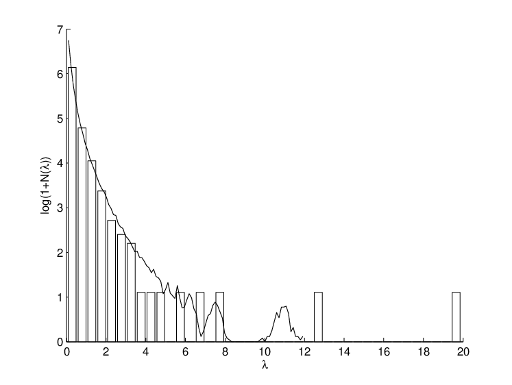
Refer to caption — Figure 1: $\log(1+N(\lambda))$ for the empirical spectrum (histogram) $N(\lambda)$ from S&P in 2004 and simulated spectrum (line). For the simulation we used log-normal distributed $\beta_{i}$ with mean 0.93, $\theta=0.26$ and log normal distributed $\gamma_{1i}$ with $\gamma_{0}=0.865$ .

From the discussion in section II.2 we expect an error on the leading eigenvalue $\lambda_{0}$ in the order of $\sqrt{2/T}$ . This does not imply the same accuracy for the eigenvector $\beta$ . To estimate the size of errors in windows of several years, we perform a Monte Carlo study based on a fairly general SVM. In a single window we assume the following returns

r_{i}(t)=\sqrt{\theta}\;\gamma_{0i}\;\eta_{t}+\sqrt{1-\theta}\;\gamma_{1i}\;\eta_{it}

(9)

Comparing equation (9) with the CAPM definition (1) we see that the first term corresponds to the market component with strength $\theta$ and the second term can be interpreted as the idiosyncratic component due to trading activity for specific stocks. For the i.i.d. noise factors we use $\eta_{t}~N(0,1)$ and $\eta_{it}~N(0,1)$ . We checked that a Laplacian noise for $\eta_{it}$ as suggested by [2] does not change the result. The parameters $\gamma_{0i}$ and $\gamma_{1i}$ are independent of time and normalized to $\sum_{i}\;\gamma_{ki}^{2}=N$ . For a window size $T\to\infty$ we get for $C$

C_{ij}=\theta\gamma_{0i}\gamma_{0j}+(1-\theta)\gamma_{1i}^{2}\;\delta_{ij}

(10)

Using perturbation theory (see the appendix) the leading eigenvalue and its eigenvector $\beta_{i}=\sqrt{N}f_{i}^{0}$ are given up to terms of order of $1/N$ by

\lambda_{0}=\theta(N-1)+1\quad\mbox{and}\quad\beta_{i}=\gamma_{0i}

(11)

$N$	log-norm.	Laplace	normal	$\gamma_{1i}=1$	T	log-norm.
100	0.109	0.109	0.108	0.125	500	0.131
200	0.107	0.109	0.110	0.124	1000	0.094
400	0.106	0.108	0.110	0.123	2000	0.066

Table 2: The left part of the table shows the average error (5% confidence level) of

\beta

T=750

for various

N

and models for

\gamma_{1}

. The right shows the error for

N=356

and log-normally distributed

\gamma_{1}

for different

T

We simulate the returns from eq. (9) with given values for $\theta$ , $\beta_{i}$ and $\gamma_{1i}$ in a finite window. From the eigenvectors of the simulated covariance matrix we can estimate the statistical error on $\beta$ due to the finite $T$ . For this we need reliable values of the input parameters. The market strength $\theta$ follows from the well measured empirical $\lambda_{0}$ . For the input $\beta_{i}$ we use a log-normal distribution, which represents the observed spectrum very well. For $\gamma_{1i}$ we choose a normal, Laplace and log-normal distribution, which depend on two parameters. Since the mean of $\gamma_{1}^{2}$ must be 1 only the mean $\gamma_{0}$ is a free parameter.

We determine $\gamma_{0}$ by optimizing the agreement of the observed eigenvalue spectrum $N(\lambda)$ with the simulated spectrum. As an example we show this comparison using $log(1+N(\lambda))$ for the S&P data in a window of 3 years around 2004 and log-normally distributed $\gamma_{1}$ . Both agree surprisingly well. A Kolmogorov-Smirnov test leads to a p-value of 0.2. In contrast, Laplace or normally distributed $\gamma_{1i}$ lead to $p\sim 10^{-4}$ or less. The model accounts apart from the bulk also for the isolated medium eigenvalues attributed in the literature to sub-markets [20, 23]. Only the second largest eigenvalue attributed to the trading volume [23] does not correspond to a statistical fluctuation.

The result of 200 Monte Carlo repetitions of the dynamic eq. (9) is shown in figure 2 for various $T$ . The ordered input $\beta_{i}$ are connected by a line. The errors correspond to a 5% confidential range for a single measurement. There is little dependence on $N$ or the assumed distribution of $\gamma_{1}$ . In table 2 we give the average error for various $N$ and different $\gamma_{1}$ and $T$ . The errors only vary with $T$ by $1/\sqrt{T}$ . These simulations prove that within the assumed SVM the values of $\beta_{i}$ can be reliably estimated also for moderate window sizes $T$ .

To summarize, for the empirical analysis of $C$ in the next section we make the following assumptions: From the market hypothesis we can establish the leading eigenvector of $C$ as CAPM $\beta$ -coefficients. By the SVM assumption the time average in eq. (2) corresponds to an average over the noise. Making the market dominance assumption the errors on $\lambda_{0}$ and $\beta_{i}$ are of the order of $1/N,\sqrt{2/T}$ .

IV Transition of the Markets in 2006

We apply our approach to 356 stocks from the S&P market, 132 stocks of the British FTSE market, and to 78 stocks from the German market. To obtain the possible minimum window size $T$ we look at the large eigenvalue $\lambda_{0}(t)$ and the corresponding eigenvector. As the criterion we use the presence of (only) positive values of $\beta_{i}(t)$ . In this way we find for $T$ a value of roughly 3-4 years for all markets. For a better visualization of the time variation we use overlapping windows by varying $t$ in steps of years.

In figure 3 we show the $\beta-$ coefficients derived from the largest eigenvector of $C$ for the S&P market for a time window of 3 years. Except one case around 2001 they are all positive. Some of the stocks exhibit a substantial time variation with a transition around 2006. Stocks with large $\beta$ during the years 1998-2002 (this time interval is called ITB for IT bubble hereafter) change to small $\beta$ values around 2006, their values remain low in 2007-2010 (this time interval is called FB for the finance bubble hereafter). Vice versa those stocks with a large $\beta$ in the finance bubble exhibit small values before 2006. A similar effect occurs also for the FTSE market (shown in figure 4) and the German market (shown in figure 5). For both a window size of 4 years is used.

R(t,s)=A_{S}\sum_{i\epsilon s}\theta(\beta_{i}-1.0)\beta_{i}(t)\;V(t,i)

(12)

The normalization constant $A_{S}$ is chosen to have $\sum_{s}\;R(t,s)=1$ .

A more detailed characterization of the market can be obtained by considering the sector $s$ out of the GICS/TRBS classification for all firms. An inspection of the firms with large $\beta$ during the ITB in figure 3 shows that they dominantly belong to the IT/technology sector. Likewise firms with large $\beta$ during the FB are mostly from the financial sector. Since a $\beta>1$ signals a risky investment, we can define a market risk measure $R(t,s)$ for the sectors by multiplying $\beta_{i}>1$ with the number $V(t,i)$ of traded shares in each window. Note that for the following analysis we merge the sectors IT and telecommunication for the UK and Germany since we have only few stocks in these sectors and they show similar behavior.

In figure 6 the risk parameters from eq. (12) for the S&P market is shown as a function of time. Only the technology sector (red) before the transition in 2006 and the financial sector (blue) after 2006 exhibit large values of the risk measure. The value of the risk measure is small for all other sectors. Due to the time window of 3 years the time of the transition can be fixed only with an error of 1.5 years. A similar phenomenon is seen for the FTSE market in figure 7 and the German market in figure 8. In contrast to the other markets the industrial sector of the DAX shows a peak in $R$ at 2006. This may be due to the fact that this sector contains one third of all firms. Some are large firms that are difficult to pinpoint to a specific sector. Since $R$ is normalized to $\sum_{s}R(t,s)=1$ , the small $R$ of technology and financials are compensated mainly by the industrial sector. The transition for the S&P appears to be somewhat sharper than for FTSE and DAX due to the smaller number of stocks in the latter.

V Explanations for the observed transition

V.1 Interpretation with a diluted Ising model

The behaviour of the risk parameter $R$ in figures 6-8 indicates a phase transition analogous to models in statistical physics with $R$ as order parameter. Such a model can be constructed by a generalization of the Ising model. There are $A$ agents trading one stock per time out of the $S$ sectors. Each agent $a$ is characterized by a spin value $\sigma_{a}$ . Values $\sigma_{a}=\pm 1$ denote trading in the risky sectors IT or financials, and $\sigma_{a}=0$ denotes the remaining $S-2$ sectors. We assume that the $\beta$ -dependent factor in eq. (12) can be replaced by its mean. Then the normalized $R(s)$ is equal to the fraction of agents trading in sector $s$ . The agents can change their opinion due to an interaction between all other agents. At each time they chose a new value of $\sigma_{a}$ by the following probabilities $w(\sigma)$

	$\displaystyle w(\pm 1)$	$\displaystyle=\frac{1}{w_{n}}\exp(\pm g(m+h))$		(13)
	$\displaystyle w(0)$	$\displaystyle=\frac{1}{w_{n}}(S-2)$		(14)

where $m\;A=\sum_{a}\sigma_{a}$ and $g$ is the strength of the interaction. $w_{n}$ normalizes the probabilities. $h$ denotes a possible external field. Since agents with $\sigma_{a}=0$ do not contribute to $m$ , the model corresponds to a dynamical dilution. For small $g$ the system is in the disordered state with $R(s)=1/S$ and for large $g$ in the ordered state with one of the $R(\pm 1)$ becoming large.

The model can be solved analytically for large agent numbers $A$ , as shown in appendix B. For $S>6$ a first order transition occurs at a critical value $g_{c}$ . An internal reason for the transition can be modeled by a dynamically changing $g$ . However, this faces the following problem: To observe a constant $R$ over 6-10 years, like for the S&P in figure 6, the time constant to change $g$ must be in the same order of magnitude. In the two years around 2006 the S&P market changes from an ordered state into a disordered and back into another ordered state, making an external reason more likely.

Reviewing possible external events around 2006 there seems to be no major political event nor any drastic change in asset prices. In fact, the volatility around that time was relatively low, as shown in the right panel of figure 9. One observes similarly high volatility before and after the transition. The only event seems to be the onset of high frequency trading (HFT) in 2005, see, e.g., [8, 10, 11]. In the left panel of figure 9 we show (as a representative example) the response time and the traded volume at the Eurex exchange. The small response time and a maximum of the trading volume hint at a growing dominance of computerized HFT trading after 2005.

There are several possibilities how HFT can trigger the transition. Faster trading may reduce the time constant in the dynamics of $g$ . Generally, computer programs might be more able than humans in hedging risks. Before 2008 they used almost riskless strategies, as arbitrage or flash trading, which became less important afterwards. In the model these effects can be accounted for by a change of $g$ or the effect of a field $h$ . If one chooses $g$ near $g_{c}$ , both phases are coexistent and only very small changes of $g$ or $h$ are needed to change the phase. In figure 10 we show a simulation of $R$ with the probabilities from eq. (13) with constant $g$ and application of a small field $h$ at $100\leq t\leq 120$ , which disfavors a previous risky sector. Obviously the model can reproduce the observed $R$ for the markets.

V.2 High frequency trading and the returns distribution

The appearance of HFT should leave traces in the distribution of returns. Advocates of HFT [11] claim that it leads to a more efficient market. More efficiency should lead to less price changes and therefore to an excess of smaller returns. Critics [28] assert that computerized trading increases instabilities, which amounts to larger returns. Both effects can be seen in the pdf for the market return $r_{M}$ . Its pdf can be characterized by the shape parameter $\alpha$ using the Pareto-Feller parametrization from eq. (8). We obtain $\alpha$ by maximizing the Log-Likelihood $L$ in each window. Errors on $\alpha$ correspond to a change of $L$ by 0.5.

In figure 11 we show the time dependence of $\alpha$ for the three markets. Before 2006 one finds values $\alpha\sim 4-5$ with good $\chi^{2}$ probabilities. For all three markets a drop to values below 3 appears after 2006. Small $\alpha$ imply a much more enhanced tail of the pdf as expected from HFT. The $\chi^{2}$ probabilities are worse in 2006, but still acceptable on the 5% level. However, the lower probabilities are due to systematic deviations from (8).

In figure 12 we show some typical pdfs of the market returns before and after 2006 for the S&P market. We see a perfect description by eq. (8) for the returns from the time windows centered in 2000 and 2002, whereas for those centered in 2008 and 2009 a substantial excess at $r\sim 0$ occurs, and the badly described tail extend to much larger value as before. This behavior is expected from HFT.

For the European markets, shown in figures 14 and 15 in the appendix, the excess of small returns is less significant. Only a significantly enlarged tail is observed after 2006. These markets might be less affected by HFT and therefore only the instability effect is seen. There is no trace in the volatility, since both effects can cancel out in $E[r^{2}]$ .

VI Conclusions

The literature on regularities in asset returns has for a long time argued that the $\beta$ values of stocks are time varying. We have shown that we can extend the concept of $\beta$ values to systematically describe a risk measure for stocks from different sectors of the economy. This slowly varying sector specific risk measure describes ordered states in the market and identifies sectors which show concentration of market risk. A possible trigger for the observed transition may be the onset of high frequency trading in 2005.

References

[1] Adcock CJ, Cortez MC, Rocha Armada MJ, Silva F (2012) Time varying betas and the unconditional distribution of asset returns. Quantitative Finance 12(6), 951–967.
[2] Alfarano S, Wagner F, Milakovic M (2008) A nonparametric approach to the noise density in stochastic volatility models. Applied Financial Economics Letters 4(5).
[3] Black F, Jensen MC, Scholes M (1972) The Capital Asset Pricing Model. Some Empirical Tests in Studies in the Theory of Capital Markets. M Jensen ed.:New York, Praeger Publishers.
[4] Beine M, Candelon B (2011) Liberalization and stock market co-movement between emerging economies. Quantitative Finance 12(2): 299–312.
[5] Bos T, Newbold P (1984) An Empirical Investigation of the Possibility of Stochastic Systemic Risk in the Market Model. The Journal of Business 57(1.1), 35–41.
[6] Bodurtha JN, Mark NC (1991) Testing the CAPM with Time-Varying Risk and Returns. The Journal of Finance 46(4), 1485–1505.
[7] Bollerslev T, Engle R, Wooldridge J (1988) A Capital Asset Pricing Model with Time-Varying Covariances. Journal of Political Economy 96(1), 116–131.
[8] Carrion A (2013) Very fast money: high-frequency trading on the NASDAQ. Journal of Financial Markets, 16(4), 680–711.
[9] Citeau P, Potters M, Bouchaud JP (2001) Correlation structure of extreme stock returns. Quantitative Finance 1, 217–222.
[10] Dichev ID, Huang K, Zhou D (2012) The Dark Side of Trading. Emory Law and Economics Research Paper No. 11-95.
[11] Ebholzer W (2014) Some insights into the details that matter for high-frequency trading! Eurex Exchange.
[12] Fama EF, French KR (1992) The Cross-Section of Expected Stock Returns. The Journal of Finance 47(2), 427–465. The Journal of Finance 46(4), 1485–1505.
[13] Harvey CJ, Siddique A (2000) Conditional Skewness in Asset Pricing Tests. The Journal of Finance LV(3), 1263–1295.
[14] Kleiber C, Kotz S (2003) Statistical Size Distributions in Economics and Actuarial Sciences, John Wiley, Hoboken, NJ.
[15] Kenett DY, Shapira Y, Madi A, Bransburg-Zabary S, Gur-Gershgoren G, Ben-Jacob E (2011) Index Cohesive Force Analysis Reveals That the US Market Became Prone to Systemic Collapses Since 2002. PLoS ONE 6(4): e19378.
[16] Kenett DY, Raddant M, Lux T, Ben-Jacob E (2012) Evolvement of Uniformity and Volatility in the Stressed Global Financial Village. PLoS ONE 7(2): e31144.
[17] Laloux L, Cizeau P, Bouchaud JP, Potters M (1999) Noise Dressing of Financial Correlation Matrices. Phys.Rev.Lett.83 1467.
[18] Lintner J (1965) The Valuation of Risk Assets and the Selection of Risky Investments in Stock Portfolios and Capital Budgets. Review of Economics and Statistics 47, 13–37.
[19] Livan G, Alfarano S, Scalas E (2011) Fine structure of spectral properties for random correlation matrices, Phys.Rev. E 84 016113.
[20] Mantegna RN (1999) Hierarchical structure in financial markets, Eur. Phys.J.B 11(1999)193.
[21] Marĉenko VA, Pastur LA (1967) Distribution of eigenvalues for some sets of random matrices. Math.USSR-Sb 1(1967)457.
[22] Münnix MC, Shimada T, Schäfer R, Leyvraz F, Seligman T, Guhr T, Stanley HE (2012) Identifying States of a Financial Market. Scientific Reports 2(644).
[23] Plerou V et al. (2002) Random matrix approach to cross correlations in financial data, Phys.Rev. E 65, 066126.
[24] Preis T, Schneider JJ, Stanley HE (2011) Switching processes in financial markets. Proceedings of the National Academy of Sciences doi:10.1073/pnas.1019484108.
[25] Raddant M, Wagner F (2013) Phase Transition in the S&P Stock Market, arXiv:1306.2508.
[26] Sharpe W (1964) Capital Asset Prices: a Theory of Market Equilibrium Under Conditions of Risk. Journal of Finance 19, 425–442.
[27] Shephard N (2005) Stochastic Volatility Models: Selected Readings. Oxford University Press, Oxford.
[28] Spence M (2011), Conference on Macro and Growth Politics in the Wake of the Crisis, Washington March 7, 2011
[29] Tumminello M, Aste T, Di Matteo T, Mantegna RN (2005) A tool for filtering information in complex systems. Proceedings of the National Academy of Sciences of the United States of America 102(30):10421-10426.

Appendix A Perturbation Theory

Assume a matrix $C$ can be written as $C=C_{0}+C_{1}$ with a small perturbation $C_{1}$ . $C_{0}$ has one large eigenvalue $E_{0}$ and $N-1$ degenerate zero eigenvalues. Due to the degeneracy we can impose for the eigenvectors $e_{i}^{\mu}$ with $\mu>0$ of $C_{0}$ the conditions

e^{\nu}\cdot(C_{1}\;e^{\mu})=0\quad\mbox{for}\quad\mu,\nu>0,\nu\neq\mu

(15)

The eigenvalues $\lambda_{\mu}$ and eigenvectors $f_{i}^{\mu}$ of $C$ can be expanded in a power serie in $C_{1}/E_{0}$ . For $\mu=0$ we get

\lambda_{0}=E_{0}+e^{0}\cdot(C_{1}\;e^{0})+\frac{1}{E_{0}}\left[e^{0}\cdot(C_{1}^{2}\;e^{0})-\left(e^{0}\cdot(C_{1}\;e^{0})\right)^{2}\right]

(16)

f_{i}^{0}=\left[1-\frac{1}{E_{0}}e^{0}\cdot(C_{1}\;e^{0})\right]e^{0}_{i}+\frac{1}{E_{0}}(C_{1}\;e^{0})_{i}

(17)

The remaining eigenvectors need the solution of condition (15)

\lambda_{\mu}=e^{\mu}\cdot(C_{1}\;e^{\mu})-\frac{1}{E_{0}}\left(e^{0}\cdot(C_{1}\;e^{\mu})\right)^{2}

(18)

f_{i}^{\mu}=e_{i}^{\mu}-\frac{1}{E_{0}}(e^{0}\cdot(C_{1}\;e^{\mu})e_{i}^{\mu}

(19)

Note that this expansion reproduces the exact result for $tr\;C$ and for $C_{1}$ proportional to a unit matrix.
With $(C_{0})_{ij}=\gamma_{i}\gamma_{j}$ we have $E_{0}=(\gamma,\gamma)=\gamma^{2}$ and $e^{0}_{i}=\gamma_{i}/\sqrt{\gamma^{2}}$ . Inserting $(\gamma,C_{1}^{k}\gamma)=A_{k}\;\gamma^{2}$ into eqns. (16) and (17) we get for $\lambda_{0}$ and $\beta_{i}=\sqrt{N}f_{i}^{0}$

\lambda_{0}=\gamma^{2}+A_{1}+\frac{1}{\gamma^{2}}(A_{2}-A_{1}^{2})

(20)

\beta_{i}=\left[1-\frac{1}{\gamma^{2}}A_{1}\right]\sqrt{\frac{N}{\gamma^{2}}}\gamma_{i}+\frac{1}{\gamma^{2}}a_{i}

(21)

with $a^{2}=(N/\gamma^{2})A_{2}$ . Market dominance implies $E_{0}=\gamma^{2}\propto N$ and the constants $A_{k}$ are of order 1. Eqns. (20) and (21) show that up to corrections of order $1/N$ the leading eigenvalue $\lambda_{0}$ and its eigenvector $\beta_{i}$ do not depend on $C_{1}$ .

Appendix B Diluted Ising Model

The transition probabilities (13) correspond to the heat bath algorithm for the following equilibrium distribution

w(\sigma)=\frac{1}{Z}\exp\left[A\cdot g(m(\sigma)^{2}/2+hm(\sigma))\right]

(22)

with $m(\sigma)=(1/A)\sum_{a}\sigma_{a}$ . The partitioned sum $Z$ we calculate by using the Gaus trick $\sqrt{\pi}\exp(m^{2})=\int dx\exp(-x^{2}+2mx)$ and evaluating the integral for large $A$ . We get for $Z$

\ln Z=A\left[\ln(S-2+2ch((m_{0}+h)g))-\frac{g}{2}m_{0}^{2}\right]

(23)

The expectation value $m_{0}$ of $m(\sigma)$ must maximize $\ln Z$ . This leads to the so called mean field condition for the order parameter $m_{0}$

m_{0}=\frac{2sh(m_{0}(g+h))}{S-2+2ch(m_{0}(g+h))}

(24)

The fraction $R_{\pm}$ at $h=0$ of agents with $\sigma_{a}=\pm 1$ is given by

R_{\pm}=\frac{\exp(\pm m_{0}g)}{S-2+2ch(m_{0}g)}

(25)

Eqns. (23) and (24) lead already at $h=0$ to a surprisingly rich spectrum of phases depending on the number of sectors $S$ and $g$ . For $S<6$ we have a similar behaviour as in the Ising model ( $S=2$ ). At $g_{c}=S/2$ a second order transition occurs. At $S=6$ the transition is still of second order, but with different critical exponents.

The general case $S>6$ is illustrated by a plot of $-\ln Z/(gA)$ in figure 13. Below $g<g_{1}$ only the disordered phase exists. At $g=g_{1}$ a $m_{0}\neq 0$ solution appears corresponding a metastable ordered phase, since $\ln Z\leq\ln Z(m_{0}=0)$ . At $g=g_{c}$ both phases coexist. For $g>g_{c}$ the $m_{0}=0$ phase becomes metastable. Finally for $g>g_{2}=S/2$ only the $m_{0}\neq 0$ solution exists. The critical values of $g$ and the values of $R(1)$ at criticality corresponding to a lower bound are given in table 3.

$S$	$g_{1}$	$g_{c}$	$g_{2}$	$R(g_{c})$
6	-	3	-	1/6
8	3.73	3.82	4	0.70
9	3.97	4.20	9/2	0.81
10	4.19	4.58	5	0.87

Table 3: Critical values of

g

and

R(g_{c})

g=g_{c}