跳到论文正文
W Papers独立论文阅读器 arXiv:1504.05745 论文正文 计算阅读时间 · 0%
引用这篇论文根据当前论文元数据生成,正式投稿前建议核对。


License: arXiv.org perpetual non-exclusive license
arXiv:1504.05745v1 [hep-th] 22 Apr 2015

Phase Transition in Tensor Models

Thibault Delepouve Note: delepouve@cpht.polytechnique.fr, Laboratoire de Physique Théorique, CNRS UMR 8627, Université Paris Sud, 91405 Orsay Cedex, France and Centre de Physique Théorique, CNRS UMR 7644, École Polytechnique, 91128 Palaiseau Cedex, France.    Razvan Gurau Note: rgurau@cpht.polytechnique.fr, Centre de Physique Théorique, CNRS UMR 7644, École Polytechnique, 91128 Palaiseau Cedex, France and Perimeter Institute for Theoretical Physics, 31 Caroline St. N, N2L 2Y5, Waterloo, ON, Canada.
Abstract

Generalizing matrix models, tensor models generate dynamical triangulations in any dimension and support a 1/N1/N expansion. Using the intermediate field representation we explicitly rewrite a quartic tensor model as a field theory for a fluctuation field around a vacuum state corresponding to the resummation of the entire leading order in 1/N1/N (a resummation of the melonic family). We then prove that the critical regime in which the continuum limit in the sense of dynamical triangulations is reached is precisely a phase transition in the field theory sense for the fluctuation field.

1 Introduction

Matrix models [1] generate dynamical triangulations and dynamical tessellations in two dimensions. Tensor models [2, 3, 4, 5, 6] generalize matrix models and generate dynamical triangulations [7, 8] in any dimension (recently a matrix model generating dynamical triangulations is dimension three has been proposed [9]). The continuum limit of dynamical triangulations is reached when tunning the coupling constants to some critical values [10, 11, 12, 13]. In this regime the number of simplices in the triangulation diverges. Sending simultaneously the volume of the individual simplices to zero one obtains a continuous phase of infinitely refined random spaces [1, 8].

Tensor and matrix models can be regarded as field theories with no kinetic term. The fields are a pair of complex conjugated tensors 𝕋a1​…​aD,𝕋¯a1​…​aD\mathbb{T}_{a^{1}\dots a^{D}},\bar{\mathbb{T}}_{a^{1}\dots a^{D}} (where ac=1,…​Na^{c}=1,\dots N) transforming under the external tensor product of DD fundamental representations of the unitary group 𝒰⁡(N){\cal U}(N):

𝕋a1​…​aD′=∑b1,…​bD=1NUa1​b1(1)​…​UaD​bD(D)​𝕋b1​…​bD,𝕋¯a1​…​aD′=∑b1,…​bD=1NU¯a1​b1(1)​…​U¯aD​bD(D)​𝕋¯b1​…​bD.\mathbb{T}^{\prime}_{a^{1}\dots a^{D}}=\sum_{b^{1},\dots b^{D}=1}^{N}U^{(1)}_{a^{1}b^{1}}\dots U^{(D)}_{a^{D}b^{D}}\mathbb{T}_{b^{1}\dots b^{D}}\;,\qquad\bar{\mathbb{T}}^{\prime}_{a^{1}\dots a^{D}}=\sum_{b^{1},\dots b^{D}=1}^{N}\bar{U}^{(1)}_{a^{1}b^{1}}\dots\bar{U}^{(D)}_{a^{D}b^{D}}\bar{\mathbb{T}}_{b^{1}\dots b^{D}}\;.

The action of tensor models is a function of 𝕋\mathbb{T} and 𝕋¯\bar{\mathbb{T}} which is invariant under unitary transformations. Like matrix models, tensor models are known to possess a 1/N1/N expansion [14, 15, 16, 17, 18]. The leading order in the 1/N1/N expansion for matrices is given by the planar triangulations. For tensor models, the leading order in 1/N1/N is given by a class of triangulations called melonic [12]. The melonic triangulations represent topological spheres in any dimensions, but one should emphasize that only a subclass of triangulations of the sphere are melonic. In particular the family of melonic triangulations is exponentially bounded [12]. It is not yet known whether the family of general triangulations of the sphere in dimension higher than three is exponentially bounded or not [19].

In this paper we consider a tensor model with a quartic interaction. We first rewrite this model, using the intermediate field representation [20, 17], as a coupled multi matrix model. Examining the vacua of this multi matrix model we find for small coupling a unique vacuum state invariant under unitary transformations which we call the melonic vacuum. We derive the effective theory for the fluctuations around the melonic vacuum. The translation to the melonic vacuum is not a phase transition as no symmetry gets broken (the melonic vacuum possesses the full invariance of the theory). We show that this translation completely resums the leading order in 1/N1/N: the effective theory for the perturbation fields around the melonic vacuum contributes only to lower orders in 1/N1/N. We show furthermore that, at each order in 1/N1/N, only a finite number of graphs of the effective theory contribute. Finally, we show that the criticality of the leading order contribution in 1/N1/N, which is the dynamical triangulation continuum limit, corresponds precisely to a zero eigenvalue in the effective mass matrix for the fluctuation field.

We therefore prove that the continuum limit in dynamical triangulations is a phase transition in tensor models. This phase transition presumably corresponds to the spontaneous breaking of the unitary invariance of the theory. In order to establish this rigorously, one needs in the future to identify the appropriate non unitary invariant vacuum state and study perturbations around it.

The situation is quite different for matrix models. A procedure similar to the one we use here for tensors can not be used for matrices: so far at least, the action of no matrix model could be translated to an explicit “planar vacuum state” such that the effective theory around it contributes only a finite number of graphs at each order in 1/N1/N.

A very interesting question is whether similar results hold for group field theories [21, 22, 23] and tensor field theories [24, 25, 26, 27, 28]. Such theories have a genuine renormalization group flow [29, 30] and it would be very interesting to test whether the phase transition we identify in this paper is associated to an infrared fixed point of this flow in which case tensor field theories and group field theories would naturally generate bound states of extended geometry.

This paper is organized as follows. As our results are somewhat technical, we start by discussing in section 2 their interpretation. In section 3 we introduce the quartic tensor model and in section 4 we discuss the effective theory around an invariant field configuration. In section 5 we introduce the class of Feynman graphs (combinatorial maps) relevant for the Feynman expansion of the effective theory which we detail in section 6. Finally in section 7 we consider the translation to the invariant vacuum state and detail the 1/N1/N expansion of the fluctuation field.

2 Discussion

The partition functions of tensor and matrix models are generating functions for dynamical triangulations [1, 7, 8]. Denoting Δ\Delta a (strongly) connected DD dimensional triangulation and Top⁡(Δ){\rm Top}(\Delta) the number of DD simplices in Δ\Delta, the logarithm of the partition function (the free energy) writes as:

W=1ND​ln⁡Z=∑ΔgTop⁡(Δ)​N−2(D−1)!​ω​(Δ),W=\frac{1}{N^{D}}\ln Z=\sum_{\Delta}\;g^{{\rm Top}(\Delta)}N^{-\frac{2}{(D-1)!}\omega(\Delta)}\;,

where NN denotes the size of the matrices (or tensors) and ω⁡(Δ)\omega(\Delta) is a non negative integer. In the case of matrices D=2D=2, ω⁡(Δ)\omega(\Delta) is the genus of the triangulations [1], while in higher dimensions [14, 16] ω⁡(Δ)\omega(\Delta) is the degree. While the degree is not a topological invariant, it serves to organize the series defining WW as a series in 1/N1/N.

In the large NN limit only a subclass of triangulations contribute: the planar triangulations in dimension two and the melonic triangulations in higher dimension. Both families are exponentially bounded. Similar results hold order by order in 1/N1/N and it can be shown that [1, 31, 32] summing the families of triangulations at fixed order in 1/N1/N, the free energy becomes (up to non universal analytic pieces in gg which can be disposed of by a suitable number of derivatives):

W∼d0​(gc−g)ν0+∑q≥11Nq​dq​(gc−g)νq.W\sim d_{0}(g_{c}-g)^{\nu_{0}}+\sum_{q\geq 1}\frac{1}{N^{q}}d_{q}(g_{c}-g)^{\nu_{q}}\;.

While the critical value gcg_{c} depends on the details of the model, all the series at fixed order in 1/N1/N become critical at the same critical value gcg_{c}. The (non integer) critical exponents ν0,νq\nu_{0},\nu_{q} are, to a large extent, universal for a given dimension.

Considering equilateral simplices of volume VDV_{D}, the physical volume of a triangulation is proportional to the number of DD simplices, and the average physical volume is:

Vol=VD⟨Top⁡(Δ)⟩=VDg∂glnW∼g→gcVDg−gc.{\rm Vol}=V_{D}\Braket{{\rm Top}(\Delta)}=V_{D}\;g\partial_{g}\ln W\sim_{g\to g_{c}}\frac{V_{D}}{g-g_{c}}\;.

The continuum limit of dynamical triangulation is reached by tuning g→gcg\to g_{c} and sending at the same time VD→0V_{D}\to 0 while keeping the average physical volume fixed. In this regime one obtains a phase of random infinitely refined geometries. One can study more involved matrix and tensor models, adding for instance coupling constants for lower dimensional simplices. The various continuum phases of the model will then be spanned by these new couplings.

Dynamical triangulations can also be studied [8, 33] with no reference to matrix and tensor models. In this case one restricts the family of triangulations by some prescription. For instance one can chose to restrict to triangulations of the sphere, or to foliated triangulations [33]. Of course one should check that the restricted family of triangulations is exponentially bounded (in order to be able to obtain a continuum limit) but, due to technical difficulties, this is never done in practice. Still, one can learn numerous lessons from numerical studies.

We show in this paper that a certain tensor model can be recast as a coupled multi matrix model for DD matrices HcH^{c}, with c=1,…​Dc=1,\dots D. We then show that, in this new formulation, the vacuum state of the model is not Hc=0H^{c}=0, but it is given at small coupling constant gg by the invariant configuration:

Hc=a0​𝟏,a0=1−1−4​D​g22​D​g.H^{c}=a_{0}{\bf 1}\;,\qquad a_{0}=\frac{1-\sqrt{1-4Dg^{2}}}{2Dg}\;.

We translate to the vacuum state and write the partition function of the model as some explicit factor multiplying the partition function of the effective theory of the perturbation fields McM^{c} around the vacuum state:

Z(4)\displaystyle Z^{(4)} =e−ND​(D​a022+ln⁡(1−g​D​a0))​(1−a02)D−12​∫[d​Mc]​e−S⁡(M),\displaystyle=e^{-N^{D}\left(\frac{Da_{0}^{2}}{2}+\ln(1-gDa_{0})\right)}(1-a_{0}^{2})^{\frac{D-1}{2}}\int[dM^{c}]\;e^{-S(M)}\;, (1)
S⁡(M)\displaystyle S(M) =12​ND−1​(1−a02)​∑c=1DTrc⁡[Mc​Mc]−12​ND−2​D−1D​a02​(∑c=1DTrc⁡[Mc])2−Q⁡(M).\displaystyle=\frac{1}{2}N^{D-1}(1-a_{0}^{2})\sum_{c=1}^{D}\Tr_{c}\left[M^{c}M^{c}\right]-\frac{1}{2}N^{D-2}\frac{D-1}{D}a_{0}^{2}\left(\sum_{c=1}^{D}\Tr_{c}[M^{c}]\right)^{2}-Q(M)\;. (2)

We prove on the one hand that the integral over the perturbation fields is subleading in 1/N1/N, namely:

−W=−1ND​ln⁡Z(4)=D2​a02+ln⁡(1−g​D​a0)+O⁡(1N),-W=-\frac{1}{N^{D}}\ln Z^{(4)}=\frac{D}{2}a_{0}^{2}+\ln(1-gDa_{0})+O\left(\frac{1}{N}\right)\;,

and on the other that the mass matrix of the effective theory for the perturbation McM^{c}, ∂2S⁡(M)∂M​∂M|M=0\frac{\partial^{2}S(M)}{\partial M\partial M}\big|_{M=0} has eigenvalues ND−1​(1−a02)N^{D-1}(1-a_{0}^{2}) with degeneracy N​D2−1ND^{2}-1 and ND−1​(1−D​a02)N^{D-1}(1-Da_{0}^{2}) with degeneracy 11.

Dynamical triangulations continuum limit. The dynamical triangulations continuum limit is obtained from the explicit factor in Eq. (1). The leading order free energy writes in terms of gg as:

−WLO=D2​a02+ln⁡(1−g​D​a0)=−12+1−1−4​D​g24​D​g2−ln⁡(1−1−4​D​g22​D​g2),\displaystyle-W_{\rm LO}=\frac{D}{2}a_{0}^{2}+\ln(1-gDa_{0})=-\frac{1}{2}+\frac{1-\sqrt{1-4Dg^{2}}}{4Dg^{2}}-\ln\left(\frac{1-\sqrt{1-4Dg^{2}}}{2Dg^{2}}\right)\;,

and becomes critical for the critical constant:

gc=12​D.\boxed{g_{c}=\frac{1}{2\sqrt{D}}\;.}

In the critical regime g2gc2=4​D​g2=1−ϵ\frac{g^{2}}{g_{c}^{2}}=4Dg^{2}=1-\epsilon one obtains:

−WLO=−12+1−ϵ1−ϵ−ln⁡(2​1−ϵ1−ϵ)=12+ln⁡2+12​ϵ−23​ϵ3/2+O⁡(ϵ2),\displaystyle-W_{\rm LO}=-\frac{1}{2}+\frac{1-\sqrt{\epsilon}}{1-\epsilon}-\ln\left(2\frac{1-\sqrt{\epsilon}}{1-\epsilon}\right)=\frac{1}{2}+\ln 2+\frac{1}{2}\epsilon-\frac{2}{3}\epsilon^{3/2}+O(\epsilon^{2})\;,

hence the critical exponent ν0=32\nu_{0}=\frac{3}{2}.

Field theory phase transition. The effective field theory for the perturbation field McM^{c} (which is subleading in 1/N1/N) undergoes a phase transition when the mass matrix has a zero eigenvalue, that is for 1−D​a02=01-Da_{0}^{2}=0. At this point the invariant vacuum is no longer stable and the symmetry of the theory is broken. This occurs for the coupling constant gp.t.g_{p.t.} solution of:

1D=1−1−4​D​gp.t.22​D​gp.t.⇒1−4​D​gp.t.2=(1−4​D​gp.t.2)⇒gp.t.=12​D.\frac{1}{\sqrt{D}}=\frac{1-\sqrt{1-4Dg_{p.t.}^{2}}}{2Dg_{p.t.}}\Rightarrow\sqrt{1-4Dg_{p.t.}^{2}}=(1-4Dg_{p.t.}^{2})\Rightarrow\boxed{g_{p.t.}=\frac{1}{2\sqrt{D}}\;.}

We conclude that, in tensor models, the dynamical triangulations continuum limit is a phase transition associated to a breaking of the symmetry (unitary symmetry and color permutation) of the model.

We stress that the phase transition we identify in this paper is of an entirely different nature form the phase transitions studied so far in the context of dynamical triangulations and matrix models:

  • •

    Dynamical triangulations. In dynamical triangulations [8, 33] one takes the continuum limit and obtains various continuum phases. In Euclidean dynamical triangulations [8] one typically obtains two continuum phases (crumpled and branched polymer), while in causal dynamical triangulations [33] one obtains three continuum phases. One is then interested in the transition between the continuum phases. These transitions have nothing to do with the phase transition from discrete to continuum we identify in this paper.

  • •

    Matrix models. In matrix models [34] one studies the transition from a one cut resolvent to a multi cut resolvent. The phase transition we identify in this paper is very different, and occurs in a completely different range of parameters. In matrix models the continuum limit is a change of behavior of the spectral density of a one cut solution (one passes from a square root law to a 3/23/2 power law for the distribution of eigenvalues). It is this change of behavior which we show in this paper is a genuine phase transition in the case of tensor models.

3 The quartic melonic model

A detailed introduction to the general framework of tensor models can be found in [13] or [35], and an introduction to the quartic melonic model in [20] and [17]. An important notion for tensor models is the notion of DD-colored graph [5]. Such graphs are dual to (D−1)(D-1)-dimensional triangulations [5].

Definition 1.

A bipartite edge DD-colored graph (DD-colored graph for short) ℬ{\cal{B}} is a graph with vertex set 𝒱⁡(ℬ){\cal{V}}({\cal{B}}) and edge set ℰ⁡(ℬ){\cal{E}}({\cal{B}}) such that:

  • •

    the vertex set 𝒱⁡(ℬ){\cal{V}}({\cal{B}}) is the disjoint union of the set 𝒱w​(ℬ){\cal{V}}^{w}({\cal{B}}) of white vertices and the set 𝒱b​(ℬ){\cal{V}}^{b}({\cal{B}}) of black vertices, with |𝒱w​(ℬ)|=|𝒱b​(ℬ)|=k⁡(ℬ)|{\cal{V}}^{w}({\cal{B}})|=|{\cal{V}}^{b}({\cal{B}})|=k({\cal{B}}).

  • •

    the edge set ℰ⁡(ℬ){\cal{E}}({\cal{B}}) is the disjoint union of DD sets ℰc​(ℬ){\cal{E}}^{c}({\cal{B}}) of edges of color cc, with c∈{1,…​D}c\in\{1,\dots D\} such that any edge connects a black and a white vertex.

  • •

    all the vertices have degree DD and all the edges incident to a vertex have distinct colors.

The fields in a tensor model are a pair of complex conjugated rank DD tensors 𝕋a1​…​aD,𝕋¯a1​…​aD{\mathbb{T}}_{a^{1}\dots a^{D}},\ \bar{\mathbb{T}}_{a^{1}\dots a^{D}}, with ac=1​…​Na^{c}=1\dots N. We call the position cc of an index its color and denote the set of colors 𝒟={1​…​D}{\cal{D}}=\{1\dots D\}. We denote a𝒟=(ac,c∈𝒟)a^{\cal{D}}=(a^{c},c\in{\cal{D}}). The tensors 𝕋\mathbb{T} and 𝕋¯\bar{\mathbb{T}} transform under the external tensor product of DD fundamental representations of the unitary group 𝒰⁡(N){\cal U}(N):

𝕋a𝒟′=∑b1,…​bD=1NUa1​b1(1)​…​UaD​bD(D)​𝕋b𝒟,𝕋¯a𝒟′=∑b1,…​bD=1NU¯a1​b1(1)​…​U¯aD​bD(D)​𝕋¯b𝒟.\mathbb{T}^{\prime}_{a^{{\cal{D}}}}=\sum_{b^{1},\dots b^{D}=1}^{N}U^{(1)}_{a^{1}b^{1}}\dots U^{(D)}_{a^{D}b^{D}}\mathbb{T}_{b^{{\cal{D}}}}\;,\qquad\bar{\mathbb{T}}^{\prime}_{a^{{\cal{D}}}}=\sum_{b^{1},\dots b^{D}=1}^{N}\bar{U}^{(1)}_{a^{1}b^{1}}\dots\bar{U}^{(D)}_{a^{D}b^{D}}\bar{\mathbb{T}}_{b^{{\cal{D}}}}\;.

Starting from 𝕋\mathbb{T} and 𝕋¯\bar{\mathbb{T}} one can build a class of invariant polynomials called trace invariants. They are in bijection with bipartite edge DD-colored graphs. The trace invariant associated to ℬ{\cal{B}} is obtained by associating to every white vertex ii of ℬ{\cal{B}} a tensor 𝕋ai𝒟\mathbb{T}_{a^{{\cal{D}}}_{i}}, to every black vertex j¯\bar{j} of ℬ{\cal{B}} a complex conjugated tensor 𝕋¯a¯j¯𝒟\bar{\mathbb{T}}_{\bar{a}^{{\cal{D}}}_{\bar{j}}} and to every edge ec=(i,j¯)e^{c}=(i,\bar{j}) of color cc of ℬ{\cal{B}}, a contraction of the indices of color cc of the two tensors associated to its end vertices ii and j¯\bar{j}:

Trℬ⁡(𝕋,𝕋¯)=(∏j=1k⁡(ℬ)𝕋aj𝒟)​(∏j¯=1k⁡(ℬ)𝕋a¯j¯𝒟)​(∏ec=(i,j¯)∈ℰ⁡(ℬ)δaic​a¯j¯c)\Tr_{{\cal{B}}}(\mathbb{T},\bar{\mathbb{T}})=\left(\prod_{j=1}^{k({\cal{B}})}\mathbb{T}_{a_{j}^{{\cal{D}}}}\right)\left(\prod_{\bar{j}=1}^{k({\cal{B}})}\mathbb{T}_{\bar{a}_{\bar{j}}^{{\cal{D}}}}\right)\left(\prod_{e^{c}=(i,\bar{j})\in{\cal{E}}({\cal{B}})}\delta_{a_{i}^{c}\bar{a}_{\bar{j}}^{c}}\right)

The melonic quartic tensor model the probability measure:

d​μ(4)\displaystyle d\mu^{(4)} =1Z(4)​(λ)​(∏n𝒟ND−1​d​𝕋¯n𝒟​d​𝕋n𝒟2​ı​π)​e−ND−1​(∑n𝒟​n¯𝒟𝕋¯n¯𝒟​δn¯𝒟​n𝒟​𝕋n𝒟−g22​∑c∈𝒟Vc(4)​(𝕋¯,𝕋)),\displaystyle=\frac{1}{Z^{(4)}(\lambda)}\left(\prod_{n^{{\cal{D}}}}N^{D-1}\frac{d\bar{\mathbb{T}}_{n^{{\cal{D}}}}d\mathbb{T}_{n^{{\cal{D}}}}}{2\imath\pi}\right)\;e^{-N^{D-1}\left(\sum_{n^{{\cal{D}}}\bar{n}^{{\cal{D}}}}\bar{\mathbb{T}}_{\bar{n}^{{\cal{D}}}}\delta_{\bar{n}^{{\cal{D}}}n^{{\cal{D}}}}\mathbb{T}_{n^{{\cal{D}}}}-\frac{g^{2}}{2}\sum_{c\in{\cal{D}}}V^{(4)}_{c}(\bar{\mathbb{T}},\mathbb{T})\right)}\;, (3)
Vc(4)​(𝕋¯,𝕋)\displaystyle V^{(4)}_{c}(\bar{\mathbb{T}},\mathbb{T}) =∑n¯𝒟​n𝒟​m𝒟​m¯𝒟(𝕋¯n¯𝒟​δn¯𝒟∖{c}​n𝒟∖{c}​𝕋n𝒟)​δn¯c​mc​δm¯c​nc​(𝕋¯m¯𝒟​δm¯𝒟∖{c}​m𝒟∖{c}​𝕋m𝒟),\displaystyle=\sum_{\bar{n}^{{\cal{D}}}n^{{\cal{D}}}m^{{\cal{D}}}\bar{m}^{{\cal{D}}}}\left(\bar{\mathbb{T}}_{\bar{n}^{{\cal{D}}}}\delta_{\bar{n}^{{\cal{D}}\setminus\{c\}}n^{{\cal{D}}\setminus\{c\}}}\mathbb{T}_{n^{{\cal{D}}}}\right)\delta_{\bar{n}^{c}m^{c}}\delta_{\bar{m}^{c}n^{c}}\left(\bar{\mathbb{T}}_{\bar{m}^{{\cal{D}}}}\delta_{\bar{m}^{{\cal{D}}\setminus\{c\}}m^{{\cal{D}}\setminus\{c\}}}\mathbb{T}_{m^{{\cal{D}}}}\right)\;, (4)

where, for any set 𝒞⊂𝒟{\cal{C}}\subset{\cal{D}}, we denote δn¯𝒞​n𝒞=∏c∈𝒞δn¯c​nc\delta_{\bar{n}^{{\cal{C}}}n^{{\cal{C}}}}=\prod_{c\in{\cal{C}}}\delta_{\bar{n}^{c}n^{c}}. The model is stable for g2<0g^{2}<0. Each invariant Vc(4)​(𝕋¯,𝕋)V^{(4)}_{c}(\bar{\mathbb{T}},\mathbb{T}) can be represented as a DD-colored graph with two white and two black vertices and signifies a gluing of four DD-simplices, two positively oriented and two negatively oriented. The coupling gg counts the number of positively oriented simplices. When evaluating the partition function in perturbation theory one obtains Feynman graphs having (D+1)(D+1) colors. Each such graph is dual to a DD-dimensional triangulation.

The generating function of the moments of μ(4)\mu^{(4)} is:

Z(4)​(J,J¯)\displaystyle Z^{(4)}(J,\bar{J}) =∫d​μ(4)​e∑𝕋¯a¯𝒟​J¯a¯𝒟+∑Ja𝒟​𝕋a𝒟,\displaystyle=\int d\mu^{(4)}\;\;e^{\sum\bar{\mathbb{T}}_{\bar{a}^{{\cal{D}}}}\bar{J}_{\bar{a}^{{\cal{D}}}}+\sum J_{a^{{\cal{D}}}}{\mathbb{T}}_{a^{{\cal{D}}}}}\;,

The partition function is the generating function at zero external sources and is denoted by Z(4)≡Z(4)​(0,0)Z^{(4)}\equiv Z^{(4)}(0,0). The cumulants (connected moments) of μ(4)\mu^{(4)} can be computed as the derivatives of the logarithm of ZZ:

κ2​k​(𝕋a1𝒟,𝕋¯a¯1¯𝒟,…​𝕋ak𝒟,𝕋¯a¯k¯𝒟)=∂(2​k)∂Ja1𝒟​∂J¯a¯1¯𝒟​…​∂Jak𝒟​∂J¯a¯k¯𝒟​ln⁡Z(4)​(J,J¯)|J=0J¯=0.\kappa_{2k}\bigl({\mathbb{T}}_{a_{1}^{{\cal{D}}}},\bar{\mathbb{T}}_{\bar{a}^{{\cal{D}}}_{\bar{1}}},\dots{\mathbb{T}}_{a^{{\cal{D}}}_{k}},\bar{\mathbb{T}}_{\bar{a}^{{\cal{D}}}_{\bar{k}}}\bigr)=\frac{\partial^{(2k)}}{\partial J_{a^{{\cal{D}}}_{1}}\partial\bar{J}_{\bar{a}^{{\cal{D}}}_{\bar{1}}}\dots\partial J_{a^{{\cal{D}}}_{k}}\partial\bar{J}_{\bar{a}^{{\cal{D}}}_{\bar{k}}}}\ln Z^{(4)}(J,\bar{J})\Big|_{\genfrac{}{}{0.0pt}{}{J =0}{\bar J =0}}\;.

The cumulants are linear combinations of trace invariant operators [35]:

κ2​k​[𝕋a1𝒟,𝕋¯a¯1¯𝒟​…​𝕋ak𝒟,𝕋¯a¯k¯𝒟]=∑ℬ,k⁡(ℬ)=k𝔎⁡(ℬ,μ(4))​∏ec=(i,j¯)∈ℰ⁡(ℬ)δaic​a¯j¯c,\kappa_{2k}[{\mathbb{T}}_{a^{{\cal{D}}}_{1}},\bar{\mathbb{T}}_{{\bar{a}}^{{\cal{D}}}_{\bar{1}}}\dots{\mathbb{T}}_{a^{{\cal{D}}}_{k}},\bar{\mathbb{T}}_{\bar{a}^{{\cal{D}}}_{\bar{k}}}]=\sum_{{\cal{B}},\;k({\cal{B}})=k}{\mathfrak{K}}({\cal{B}},\mu^{(4)})\prod_{e^{c}=(i,\bar{j})\in{\cal{E}}({\cal{B}})}\delta_{a^{c}_{i}\bar{a}_{\bar{j}}^{c}}\;,

where the sum runs over all the DD-colored graphs [5] ℬ{\cal{B}} with k⁡(ℬ)k({\cal{B}}) white vertices. Somewhat abusively, we call the coefficient 𝔎⁡(ℬ,μ(4)){\mathfrak{K}}({\cal{B}},\mu^{(4)}) also a cumulant and we define the rescaled cumulant corresponding to the graph ℬ{\cal{B}}:

K⁡(ℬ,μ(4))≡𝔎⁡(ℬ,μ(4))ND−2​k​(ℬ)​(D−1)−C⁡(ℬ),K({\cal{B}},\mu^{(4)})\equiv\frac{{\mathfrak{K}}({\cal{B}},\mu^{(4)})}{N^{D-2k({\cal{B}})(D-1)-C({\cal{B}})}}\;,

where C⁡(ℬ)C({\cal{B}}) denotes the number of connected components of ℬ{\cal{B}}.

3.1 The intermediate field representation

The intermediate field representation of the quartic melonic models has already been discussed in detail in [20] and [17]. Let us recall here the main steps in its derivation. Each quartic interaction in expressed in the intermediate field (Hubbard Stratonovich) representation as an integral over an auxiliary N×NN\times N hermitian matrix:

eND−1​g22​∑c∈𝒟Vc(4)​(𝕋¯,𝕋)=∫[d​Hc]​e−12​ND−1​Tr⁡[Hc​Hc]+g​ND−1​∑nc​n¯cHn¯c​ncc​∑n𝒟∖{c}​n¯𝒟∖{c}(𝕋¯n¯𝒟​δn¯𝒟∖{c}​n𝒟∖{c}​𝕋n𝒟),e^{N^{D-1}\frac{g^{2}}{2}\sum_{c\in{\cal{D}}}V^{(4)}_{c}(\bar{\mathbb{T}},\mathbb{T})}=\int[dH_{c}]\;e^{-\frac{1}{2}N^{D-1}\Tr[H^{c}H^{c}]+gN^{D-1}\sum_{n^{c}\bar{n}^{c}}H^{c}_{\bar{n}^{c}n^{c}}\sum_{n^{{\cal{D}}\setminus\{c\}}\bar{n}^{{\cal{D}}\setminus\{c\}}}\left(\bar{\mathbb{T}}_{\bar{n}^{{\cal{D}}}}\delta_{\bar{n}^{{\cal{D}}\setminus\{c\}}n^{{\cal{D}}\setminus\{c\}}}\mathbb{T}_{n^{{\cal{D}}}}\right)}\;,

where the integral over HcH^{c} is normalized to 11 for g=0g=0. As there are DD quartic melonic interactions, one obtains DD intermediate matrix fields HcH^{c}. Each HcH^{c} is an N×NN\times N matrix and the indices of HcH^{c} have the color cc. The integral over 𝕋\mathbb{T} and 𝕋¯\bar{\mathbb{T}} is now Gaussian and can be computed explicitly to obtain:

Z(4)​(J,J¯)\displaystyle Z^{(4)}(J,\bar{J}) =∫(∏c=1D[d​Hc])​e−S⁡(H)+1ND−1​J​R​(H)​J¯,\displaystyle=\int\left(\prod_{c=1}^{D}[dH^{c}]\right)e^{-S(H)+\frac{1}{N^{D-1}}JR(H)\bar{J}}\;,
S⁡(H)\displaystyle S(H) =12​ND−1​∑c=1DTrc⁡[Hc​Hc]−Tr𝒟⁡[ln⁡R⁡(H)],\displaystyle=\frac{1}{2}N^{D-1}\sum_{c=1}^{D}\Tr_{c}[H^{c}H^{c}]-\Tr_{{\cal{D}}}\left[\ln R(H)\right]\;,

where Trc\Tr_{c} is the trace over the index of color cc, Tr𝒟\Tr_{{\cal{D}}} is the trace over all the indices, and the resolvent is:

R⁡(H)=1𝟏𝒟−g​∑c=1DHc⊗𝟏𝒟∖{c},R(H)=\frac{1}{{\bf 1}^{{\cal{D}}}-g\sum_{c=1}^{D}H^{c}\otimes{\bf 1}^{{\cal{D}}\setminus\{c\}}}\;,

where 𝟏c{\bf 1}^{c} is the identity matrix with indices of color cc and for any subset 𝒞⊂𝒟{\cal{C}}\subset{\cal{D}} we denote 𝟏𝒞=⨂c∈𝒞𝟏c{\bf 1}^{{\cal{C}}}=\bigotimes_{c\in{\cal{C}}}{\bf 1}^{c}.

In the rest of this paper gg will be considered real, positive, and smaller than 12​D\frac{1}{2\sqrt{D}}. Observe that in this range of the coupling constant the resolvent can be singular. However one can still make sense of the integral defining Z(4)​(J,J¯)Z^{(4)}(J,\bar{J}) by modifying the contour of integration for the field HcH^{c} in the complex plane so as to avoid the singularities.

3.2 Equations of motion

Taking into account that:

∂∂Ha¯c​bcc​Tr𝒟​[ln⁡R⁡(H)]=g​∑p¯𝒟​q𝒟R​(H)q𝒟​p¯𝒟​(δp¯𝒟∖{c}​q𝒟∖{c}​δp¯c​a¯c​δqc​bc),\frac{\partial}{\partial H^{c}_{\bar{a}^{c}b^{c}}}\Tr_{{\cal{D}}}\left[\ln R(H)\right]=g\;\sum_{\bar{p}^{{\cal{D}}}q^{{\cal{D}}}}R(H)_{q^{{\cal{D}}}\bar{p}^{{\cal{D}}}}\left(\delta_{\bar{p}^{{\cal{D}}\setminus\{c\}}q^{{\cal{D}}\setminus\{c\}}}\delta_{\bar{p}^{c}\bar{a}^{c}}\delta_{q^{c}b^{c}}\right)\;,

the classical equations of motion in the intermediate field representation write:

0=∂S⁡(H)∂Hbc​acc=ND−1​Hac​bcc−g​∑p𝒟​q𝒟R​(H)q𝒟​p𝒟​(δp𝒟∖{c}​q𝒟∖{c}​δpc​bc​δqc​ac).0=\frac{\partial S(H)}{\partial H^{c}_{b^{c}a^{c}}}=N^{D-1}H^{c}_{a^{c}b^{c}}-g\;\sum_{p^{{\cal{D}}}q^{{\cal{D}}}}R(H)_{q^{{\cal{D}}}p^{{\cal{D}}}}\left(\delta_{p^{{\cal{D}}\setminus\{c\}}q^{{\cal{D}}\setminus\{c\}}}\delta_{p^{c}b^{c}}\delta_{q^{c}a^{c}}\right)\;.

The Hc=0H^{c}=0 configuration is not a vacuum of the theory as, for g≠0g\neq 0, Hc=0H^{c}=0 is not a solution of the classical equations of motion. In order to find solutions to the classical equations of motion we express them in matrix form:

Hc−g​1ND−1​Tr𝒟∖{c}​[1𝟏𝒟−g​∑c′=1DHc′⊗𝟏𝒟∖{c′}]=0,H^{c}-g\frac{1}{N^{D-1}}\Tr_{{\cal{D}}\setminus\{c\}}\left[\frac{1}{{\bf 1}^{{\cal{D}}}-g\sum_{c^{\prime}=1}^{D}H^{c^{\prime}}\otimes{\bf 1}^{{\cal{D}}\setminus\{c^{\prime}\}}}\right]=0\;, (5)

where Tr𝒟∖{c}\Tr_{{\cal{D}}\setminus\{c\}} denotes the trace over the indices with colors in 𝒟∖{c}{\cal{D}}\setminus\{c\}. A simple inspection of these equations reveals that for gg small enough the stable vacuum of the theory is invariant under conjugation by the unitary group and invariant under color permutation, Hc=a​𝟏H^{c}=a{\bf 1}. The invariant solutions of eq. (5) are then obtained for aa satisfying the self consistency equation:

a=g1−g​D​a.a=\frac{g}{1-gDa}\;.

This self consistency equation has two solutions:

  • •

    The melonic vacuum. A first solution, denoted a0a_{0} and called the melonic vacuum, is the sum of a power series in gg:

    a0=1−1−4​D​g22​g​D=g​∑n≥01(n+1)!​(2​nn)​(D​g2)n.a_{0}=\frac{1-\sqrt{1-4Dg^{2}}}{2gD}=g\sum_{n\geq 0}\frac{1}{(n+1)!}\binom{2n}{n}(Dg^{2})^{n}\;.

    We will see below that this solution is the stable vacuum of the theory for gg small enough. In the region of interest (g∈ℝ+, 4​D​g2<1g\in\mathbb{R_{+}},\;4Dg^{2}<1), a0a_{0} is real, positive, and bounded by:

    a0=1−1−4​D​g22​D​g=2​g1+1−4​D​g2≤1D,a_{0}=\frac{1-\sqrt{1-4Dg^{2}}}{2Dg}=\frac{2g}{1+\sqrt{1-4Dg^{2}}}\leq\frac{1}{\sqrt{D}}\;,

    as 2​g1+1−4​D​g2\frac{2g}{1+\sqrt{1-4Dg^{2}}} is increasing with gg and attains its maximum for g=12​Dg=\frac{1}{2\sqrt{D}}.

  • •

    The instanton. The second solution, denoted ainsta_{\rm inst}, is an instanton solution:

    ainst=1+1−4​D​g22​g​D.a_{\rm inst}=\frac{1+\sqrt{1-4Dg^{2}}}{2gD}\;.

    As a0​ainst=1Da_{0}a_{\rm inst}=\frac{1}{D}, it follows that in the region of interest (g∈ℝ+, 4​D​g2<1g\in\mathbb{R_{+}},\;4Dg^{2}<1), ainsta_{\rm inst} is real, positive, and ainst≥1Da_{\rm inst}\geq\frac{1}{\sqrt{D}}.

For g=12​Dg=\frac{1}{2\sqrt{D}} the two solutions collapse: a0|g=12​D=ainst|g=12​D=1Da_{0}|_{g=\frac{1}{2\sqrt{D}}}=a_{\rm inst}|_{g=\frac{1}{2\sqrt{D}}}=\frac{1}{\sqrt{D}}.

4 Translating the intermediate field

In order to study the effective theory around a solution of the classical equations of motion we must translate the field to Hc=a​𝟏+McH^{c}=a\mathbf{1}+M^{c}. This translation is a translation (in the complex plane) by aa of the contour of integration of all the diagonal entries of HcH^{c}. The effective theory is obtained by Taylor expanding in McM^{c}. We first discuss a translation of HcH^{c} by some arbitrary constant aa. We denote M=∑c=1DMc⊗𝟏𝒟∖{c}M=\sum_{c=1}^{D}M^{c}\otimes{\bf 1}^{{\cal{D}}\setminus\{c\}} and we define:

b⁡(a)≡g1−g​D​a.b(a)\equiv\frac{g}{1-gDa}\;.

Observe that if gg is real and aa is real, then b⁡(a)b(a) is also real. The melonic vacuum and the instanton are the two solutions of the self consistency equation a=b⁡(a)a=b(a). We will use the shorthand notation bb instead of b⁡(a)b(a) but the reader should keep in mind that bb is a function of aa.

In terms of the perturbation field MM, the resolvent and the trace of its logarithm write as:

R⁡(a​𝟏𝒟+M)=1(1−g​D​a)​𝟏𝒟−g​M=(11−g​D​a)​1𝟏𝒟−b​M,\displaystyle R(a\mathbf{1}^{{\cal{D}}}+M)=\frac{1}{(1-gDa)\mathbf{1}^{{\cal{D}}}-gM}=\left(\frac{1}{1-gDa}\right)\frac{1}{\mathbf{1}^{{\cal{D}}}-bM}\;,
Tr𝒟⁡[ln⁡R⁡(a​𝟏𝒟+M)]=−ND​ln⁡(1−g​D​a)+Tr𝒟⁡[ln⁡1𝟏𝒟−b​M].\displaystyle\Tr_{{\cal{D}}}\left[\ln R(a\mathbf{1}^{{\cal{D}}}+M)\right]=-N^{D}\ln(1-gDa)+\Tr_{{\cal{D}}}\left[\ln\frac{1}{\mathbf{1}^{{\cal{D}}}-bM}\right]\;.

After translation by aa the action becomes:

12​ND​D​a2+ND−1​a​∑c=1DTrc⁡[Mc]+12​ND−1​∑c=1DTrc⁡[Mc​Mc]+ND​ln⁡(1−g​D​a)−Tr𝒟⁡[ln⁡1𝟏𝒟−b​M],\displaystyle\frac{1}{2}N^{D}Da^{2}+N^{D-1}a\sum_{c=1}^{D}\Tr_{c}[M^{c}]+\frac{1}{2}N^{D-1}\sum_{c=1}^{D}\Tr_{c}[M^{c}M^{c}]+N^{D}\ln(1-gDa)-\Tr_{{\cal{D}}}\left[\ln\frac{1}{\mathbf{1}^{{\cal{D}}}-bM}\right]\;,

and the generating function writes in terms of the perturbation field MM:

Z(4)​(J,J¯)\displaystyle Z^{(4)}(J,\bar{J}) =e−ND​(D​a22+ln⁡(1−g​D​a))\displaystyle=e^{-N^{D}\left(\frac{Da^{2}}{2}+\ln(1-gDa)\right)}
×∫(∏c=1D[dMc])e−ND−12∑c=1DTrc[McMc]−aTr𝒟[M]+Tr𝒟[ln1𝟏𝒟−b​M]+1ND−11(1−g​D​a)J(1𝟏𝒟−b​M)J¯.\displaystyle\qquad\times\int\left(\prod_{c=1}^{D}[dM^{c}]\right)e^{-\frac{N^{D-1}}{2}\sum_{c=1}^{D}\Tr_{c}[M^{c}M^{c}]-a\Tr_{{\cal{D}}}[M]+\Tr_{{\cal{D}}}\left[\ln\frac{1}{\mathbf{1}^{{\cal{D}}}-bM}\right]+\frac{1}{N^{D-1}}\frac{1}{(1-gDa)}J\left(\frac{1}{\mathbf{1}^{{\cal{D}}}-bM}\right)\bar{J}}\;.

The logarithm of the resolvent contains quadratic terms in MM, which must be reabsorbed in the quadratic part of the action. Let us define the subtracted vertex function:

Q⁡(M)=Tr𝒟⁡[ln⁡1𝟏𝒟−b​M]−Tr𝒟⁡[a​M]−12​Tr𝒟​[(b​M)2],Q(M)=\Tr_{{\cal{D}}}\left[\ln\frac{1}{\mathbf{1}^{{\cal{D}}}-bM}\right]-\Tr_{{\cal{D}}}\left[aM\right]-\frac{1}{2}\Tr_{{\cal{D}}}\left[\big(bM\big)^{2}\right]\;,

which, by definition, has no quadratic terms in MM. The generating function is then:

Z(4)​(J,J¯)\displaystyle Z^{(4)}(J,\bar{J}) =e−ND​(D​a22+ln⁡(1−g​D​a))\displaystyle=e^{-N^{D}\left(\frac{Da^{2}}{2}+\ln(1-gDa)\right)}
×∫(∏c=1D[dMc])e−ND−12∑c=1DTrc[McMc]+12Tr𝒟[(bM)2]+Q(M)+1ND−11(1−g​D​a)J(1𝟏𝒟−b​M)J¯.\displaystyle\qquad\times\int\left(\prod_{c=1}^{D}[dM^{c}]\right)e^{-\frac{N^{D-1}}{2}\sum_{c=1}^{D}\Tr_{c}[M^{c}M^{c}]+\frac{1}{2}\Tr_{{\cal{D}}}\left[\big(bM\big)^{2}\right]+Q(M)+\frac{1}{N^{D-1}}\frac{1}{(1-gDa)}J\left(\frac{1}{\mathbf{1}^{{\cal{D}}}-bM}\right)\bar{J}}\;. (6)
Integral form of the subtracted vertex function.

One can give a closed integral formula for the subtracted vertex function Q⁡(M)Q(M). A Taylor expansion with integral rest yields:

Tr𝒟⁡[ln⁡1𝟏𝒟−b​M]=\displaystyle\Tr_{{\cal{D}}}\left[\ln\frac{1}{\mathbf{1}^{{\cal{D}}}-bM}\right]=
={∂tTr𝒟⁡[ln⁡1𝟏𝒟−t​b​M]}t=0+12​{∂t2Tr𝒟⁡[ln⁡1𝟏𝒟−t​b​M]}t=0+12​∫01d​t​(1−t)2​∂t3Tr𝒟⁡[ln⁡1𝟏𝒟−t​b​M],\displaystyle\qquad=\left\{\partial_{t}\Tr_{{\cal{D}}}\left[\ln\frac{1}{\mathbf{1}^{{\cal{D}}}-tbM}\right]\right\}_{t=0}+\frac{1}{2}\left\{\partial^{2}_{t}\Tr_{{\cal{D}}}\left[\ln\frac{1}{\mathbf{1}^{{\cal{D}}}-tbM}\right]\right\}_{t=0}+\frac{1}{2}\int_{0}^{1}dt\;(1-t)^{2}\partial^{3}_{t}\Tr_{{\cal{D}}}\left[\ln\frac{1}{\mathbf{1}^{{\cal{D}}}-tbM}\right]\;,

and substituting the derivatives:

∂trTr𝒟⁡[ln⁡1𝟏𝒟−t​b​M]=(r−1)!​Tr𝒟​[1(𝟏𝒟−t​b​M)r​(b​M)r],\partial_{t}^{r}\Tr_{{\cal{D}}}\left[\ln\frac{1}{\mathbf{1}^{{\cal{D}}}-tbM}\right]=(r-1)!\Tr_{{\cal{D}}}\left[\frac{1}{(\mathbf{1}^{{\cal{D}}}-tbM)^{r}}\big(bM\big)^{r}\right]\;,

we obtain:

Q⁡(M)=(b−a)​Tr𝒟​[M]+∫01d​t​(1−t)2​Tr𝒟​[1(𝟏𝒟−t​b​M)3​(b​M)3],Q(M)=(b-a)\Tr_{{\cal{D}}}\left[M\right]+\int_{0}^{1}dt\;(1-t)^{2}\Tr_{{\cal{D}}}\left[\frac{1}{(\mathbf{1}^{{\cal{D}}}-tbM)^{3}}\big(bM\big)^{3}\right]\;,

that is Q⁡(M)Q(M) is the sum of a linear piece and a piece starting at order M3M^{3}.

Linear term.

At the price of modifying the covariance, the translation of HcH^{c} by a generic aa introduces some univalent vertices in the theory. Choosing a=a0a=a_{0} comes to choosing the weight of the univalent vertex as the counterterm of the melonic graphs [12, 13], and by translating to the melonic vacuum, one subtracts the contribution of the entire melonic family: as a0=b⁡(a0)a_{0}=b(a_{0}), the linear term (b−a)​Tr𝒟​[M]\big(b-a\big)\Tr_{{\cal{D}}}[M] which represents the univalent vertices vanishes. As expected, in this case Mc=0M^{c}=0 is a solution of the classical equations of motion due to the fact that the remaining piece of Q⁡(M)Q(M) starts at order M3M^{3}.

No such interpretation exists for the translation to the instanton ainsta_{\rm inst} although the linear term cancels also in that case.

Free energy.

We can compute the large NN free energy of the model in the perturbative regime using Schwinger Dyson equations. According to [13], the large NN covariance K2K_{2} and the large NN free energy are:

1−K2+D​g2​K22=0⇒K2=1−1−4​D​g22​D​g2=a0g,\displaystyle 1-K_{2}+Dg^{2}K_{2}^{2}=0\ \Rightarrow\ K_{2}=\frac{1-\sqrt{1-4Dg^{2}}}{2Dg^{2}}=\frac{a_{0}}{g}\;,
W∞=limN→∞(1ND​ln⁡Z(4)​(0,0))=1+ln⁡(K2)−K2+D​g22​K22=−D​g22​K22+ln⁡(K2).\displaystyle W_{\infty}=\lim_{N\to\infty}\left(\frac{1}{N^{D}}\ln Z^{(4)}(0,0)\right)=1+\ln(K_{2})-K_{2}+\frac{Dg^{2}}{2}K_{2}^{2}=-\frac{Dg^{2}}{2}K_{2}^{2}+\ln(K_{2})\;.

The large NN free energy writes in term of a0a_{0} as:

W∞=−D2​a02−ln⁡(1−g​D​a0),W_{\infty}=-\frac{D}{2}a_{0}^{2}-\ln(1-gDa_{0})\;,

that is precisely the explicit prefactor in Eq. (6) for a=a0a=a_{0}. We will re-derive this result below.

It ensues that the translation to the melonic vacuum Hc=a0​𝟏H^{c}=a_{0}\mathbf{1} resums the contribution of the melonic sector, and the remaining integral over MM (which, as we will see below, only contributes at lower orders in 1/N1/N) is precisely the effective theory of a perturbation field around the melonic phase.

We note that the case of matrices, D=2D=2, is quite different. A careful inspection shows that for matrices, even after translating to a=a0a=a_{0}, the integral over the perturbation MM contributes at leading order in 1/N1/N. This is natural because for matrices the melonic graphs are only a subset of the planar graphs, and one cannot subtract the contribution of the planar sector by a single counterterm.

4.1 The effective theory for the fluctuation field

The space of Hermitian N×NN\times N matrices is a N2N^{2} dimensional real vector space ℋ{\cal H} with inner product ⟨A|B⟩≡Tr⁡[A​B]\Braket{A|B}\equiv\Tr[AB]. The quadratic part of the action is a quadratic form on the direct sum of DD such Hilbert spaces ⨁c=1Dℋc\bigoplus_{c=1}^{D}{\cal{H}}^{c}. Denoting a generic element in this direct sum space by:

M^=(M1MD),\hat{M}=\begin{pmatrix}M^{1}\\ \vdots\\ M^{D}\end{pmatrix}\;,

the inner product in ⨁c=1Dℋc\bigoplus_{c=1}^{D}{\cal{H}}^{c} is:

⟨P^|M^⟩=∑c=1DTrc⁡[Pc​Mc].\Braket{\hat{P}|\hat{M}}=\sum_{c=1}^{D}\Tr_{c}[P^{c}M^{c}]\;.

The effective theory for the fluctuation field M^\hat{M} is somewhat involved due to the fact that, while the quadratic part of the action is a quadratic form on the direct sum space ⨁c=1Dℋc\bigoplus_{c=1}^{D}{\cal{H}}^{c}, the interaction Q⁡(M)Q(M) is a trace in the tensor product space ⨂c=1Dℋc\bigotimes_{c=1}^{D}{\cal{H}}^{c}. This is the root of all the subtleties we will need to deal with below.

We now work out the effective covariance for the fluctuation field. The quadratic part of the action of the fluctuation field in Eq. (6) is:

ND−1​∑c=1DTrc⁡[Mc​Mc]−Tr𝒟⁡[(b​M)2]=\displaystyle N^{D-1}\sum_{c=1}^{D}\Tr_{c}[M^{c}M^{c}]-\Tr_{{\cal{D}}}[(bM)^{2}]=
=ND−1​(1−b2)​∑c=1DTrc⁡[(Mc)2]+ND−2​b2​∑c=1D(Trc⁡[Mc])2−ND−2​b2​(∑c=1DTrc⁡[Mc])2.\displaystyle\qquad=N^{D-1}(1-b^{2})\sum_{c=1}^{D}\Tr_{c}[(M^{c})^{2}]+N^{D-2}b^{2}\sum_{c=1}^{D}\Big(\Tr_{c}[M^{c}]\Big)^{2}-N^{D-2}b^{2}\left(\sum_{c=1}^{D}\Tr_{c}[M^{c}]\right)^{2}\;.

We denote by I^c\hat{I}_{c} the element of ⨁c=1Dℋc\bigoplus_{c=1}^{D}{\cal{H}}^{c} consisting in the identity matrix in ℋc{\cal H}^{c} and zero on the other components and by I^\hat{I} the element consisting in the identity matrix in all the ℋc{\cal H}^{c}s:

I^c=(0𝟏0),I^=(𝟏𝟏)=∑c=1DI^c.\hat{I}_{c}=\begin{pmatrix}0\\ \vdots\\ {\bf 1}\\ \vdots\\ 0\end{pmatrix}\;,\quad\hat{I}=\begin{pmatrix}{\bf 1}\\ \vdots\\ {\bf 1}\end{pmatrix}=\sum_{c=1}^{D}\hat{I}_{c}\;.

The orthogonal projectors on the one dimensional subspaces generated by I^c\hat{I}_{c} and I^\hat{I} are:

𝐏c​M^\displaystyle{\bf P}_{c}\;{\hat{M}} =⟨I^c|M^⟩⟨I^c|I^c⟩​I^c=Trc⁡[Mc]N​I^c⇒⟨M^|𝐏c​M^⟩=Trc⁡[Mc]N​Trc​[Mc]\displaystyle=\frac{\Braket{{\hat{I}}_{c}|{\hat{M}}}}{\Braket{{\hat{I}}_{c}|{\hat{I}}_{c}}}{\hat{I}}_{c}=\frac{\Tr_{c}[M^{c}]}{N}{\hat{I}}_{c}\Rightarrow\Braket{{\hat{M}}|{\bf P}_{c}\;{\hat{M}}}=\frac{\Tr_{c}[M^{c}]}{N}\Tr_{c}[M^{c}]
𝐏​M^\displaystyle{\bf P}{\hat{M}} =⟨I^|M^⟩⟨I^|I^⟩​I^=∑c=1DTrc⁡[Mc]D​N​I^⇒⟨M^|𝐏​M^⟩=∑c=1DTrc⁡[Mc]D​N​(∑c′=1DTrc′⁡[Mc′]).\displaystyle=\frac{\Braket{{\hat{I}}|{\hat{M}}}}{\Braket{{\hat{I}}|{\hat{I}}}}{\hat{I}}=\frac{\sum_{c=1}^{D}\Tr_{c}[M^{c}]}{DN}{\hat{I}}\Rightarrow\Braket{{\hat{M}}|{\bf P}{\hat{M}}}=\frac{\sum_{c=1}^{D}\Tr_{c}[M^{c}]}{DN}\left(\sum_{c^{\prime}=1}^{D}\Tr_{c^{\prime}}[M^{c^{\prime}}]\right)\;.

Let us denote 𝐈{\bf I} the identity operator on ⨁c=1Dℋc\bigoplus_{c=1}^{D}{\cal{H}}^{c}. The quadratic part writes then as ⟨M^|𝐎​M^⟩\Braket{\hat{M}|{\bf O}\;\hat{M}} where the operator 𝐎{\bf O} is:

𝐎=ND−1​(1−b2)​𝐈+ND−1​b2​∑c=1D𝐏c−ND−1​D​b2​𝐏.{\bf O}=N^{D-1}(1-b^{2})\;{\bf I}+N^{D-1}b^{2}\sum_{c=1}^{D}{\bf P}_{c}-N^{D-1}Db^{2}\;{\bf P}\;.

The covariance of the effective theory is the operator 𝐎−1{\bf O}^{-1}. In order to compute it, it is most convenient to diagonalize 𝐎{\bf O}.

Lemma 1.

The operator 𝐎{\bf O} is diagonalized as:

𝐎=ND−1​(1−b2)​[𝐈−∑c=1D𝐏c]+ND−1​[∑c=1D𝐏c−𝐏]+ND−1​(1−D​b2)​𝐏,{\bf O}=N^{D-1}(1-b^{2})\left[{\bf I}-\sum_{c=1}^{D}{\bf P}_{c}\right]+N^{D-1}\left[\sum_{c=1}^{D}{\bf P}_{c}-{\bf P}\right]+N^{D-1}(1-Db^{2}){\bf P}\;,

where 𝐈−∑c=1D𝐏c{\bf I}-\sum_{c=1}^{D}{\bf P}_{c}, ∑c=1D𝐏c−𝐏\sum_{c=1}^{D}{\bf P}_{c}-{\bf P} and 𝐏{\bf P} are the projectors on the eigenspaces of 𝐎{\bf O}. The eigenvalues of 𝐎{\bf O} and their degeneracies are:

Λ1=ND−1​(1−b2)\displaystyle\Lambda_{1}=N^{D-1}(1-b^{2})\; ,dim(Im[𝐈−∑c=1D𝐏c])=DN2−D,\displaystyle,\quad{\rm dim}\left({\rm Im}\left[{\bf I}-\sum_{c=1}^{D}{\bf P}_{c}\right]\right)=DN^{2}-D\;,
Λ2=ND−1\displaystyle\Lambda_{2}=N^{D-1}\; ,dim(Im[∑c=1D𝐏c−𝐏])=D−1,\displaystyle,\quad{\rm dim}\left({\rm Im}\left[\sum_{c=1}^{D}{\bf P}_{c}-{\bf P}\right]\right)=D-1\;,
Λ3=ND−1​(1−D​b2)\displaystyle\Lambda_{3}=N^{D-1}(1-Db^{2})\; ,dim(Im[𝐏])=1.\displaystyle,\quad{\rm dim}\left({\rm Im}\left[{\bf P}\right]\right)=1\;.
Proof.

It is enough to check that the operators 𝐈−∑c=1D𝐏c{\bf I}-\sum_{c=1}^{D}{\bf P}_{c}, ∑c=1D𝐏c−𝐏\sum_{c=1}^{D}{\bf P}_{c}-{\bf P} and 𝐏{\bf P} are three (mutually orthogonal) orthogonal projections. The three operators are obviously Hermitian and:

𝐏c′​𝐏c​M^=Trc⁡[Mc]N​⟨I^c′|I^c⟩N​I^c′=δc​c′​𝐏c​M^,\displaystyle{\bf P}_{c^{\prime}}{\bf P}_{c}\hat{M}=\frac{\Tr_{c}[M^{c}]}{N}\frac{\Braket{\hat{I}_{c^{\prime}}|\hat{I}_{c}}}{N}\hat{I}_{c^{\prime}}=\delta_{cc^{\prime}}{\bf P}_{c}\hat{M}\;,
(∑c=1D𝐏c)​𝐏​M^=∑c′=1DTrc′⁡[Mc′]D​N​∑c=1D⟨I^c|I⟩N​I^c=𝐏​M^,\displaystyle\left(\sum_{c=1}^{D}{\bf P}_{c}\right){\bf P}\hat{M}=\frac{\sum_{c^{\prime}=1}^{D}\Tr_{c^{\prime}}[M^{c^{\prime}}]}{DN}\sum_{c=1}^{D}\frac{\Braket{\hat{I}_{c}|I}}{N}\hat{I}_{c}={\bf P}\hat{M}\;,
𝐏⁡(∑c=1D𝐏c)​M^=∑c=1DTrc⁡[Mc]N​⟨I^|I^c⟩D​N​I^=𝐏​M^.\displaystyle{\bf P}\left(\sum_{c=1}^{D}{\bf P}_{c}\right)\hat{M}=\sum_{c=1}^{D}\frac{\Tr_{c}[M^{c}]}{N}\frac{\Braket{{\hat{I}}|{\hat{I}}_{c}}}{DN}{\hat{I}}={\bf P}\hat{M}\;.

The rest of the proof is a straightforward computation:

[𝐈−∑c=1D𝐏c]​[𝐈−∑c=1D𝐏c]\displaystyle\left[{\bf I}-\sum_{c=1}^{D}{\bf P}_{c}\right]\left[{\bf I}-\sum_{c=1}^{D}{\bf P}_{c}\right] =𝐈−2​∑c=1D𝐏c+∑c,c′=1D𝐏c​𝐏c′=𝐈−∑c=1D𝐏c,\displaystyle={\bf I}-2\sum_{c=1}^{D}{\bf P}_{c}+\sum_{c,c^{\prime}=1}^{D}{\bf P}_{c}{\bf P}_{c^{\prime}}={\bf I}-\sum_{c=1}^{D}{\bf P}_{c}\;,
[∑c=1D𝐏c−𝐏]​[∑c=1D𝐏c−𝐏]\displaystyle\left[\sum_{c=1}^{D}{\bf P}_{c}-{\bf P}\right]\left[\sum_{c=1}^{D}{\bf P}_{c}-{\bf P}\right] =∑c,c′=1D𝐏c​𝐏c′−𝐏⁡(∑c=1D𝐏c)−(∑c=1D𝐏c)​𝐏+𝐏\displaystyle=\sum_{c,c^{\prime}=1}^{D}{\bf P}_{c}{\bf P}_{c^{\prime}}-{\bf P}\left(\sum_{c=1}^{D}{\bf P}_{c}\right)-\left(\sum_{c=1}^{D}{\bf P}_{c}\right){\bf P}+{\bf P}
=∑c=1D𝐏c−𝐏,\displaystyle=\sum_{c=1}^{D}{\bf P}_{c}-{\bf P}\;,
𝐏2\displaystyle{\bf P}^{2} =𝐏,\displaystyle={\bf P}\;,
[𝐈−∑c=1D𝐏c]​[∑c=1D𝐏c−𝐏]\displaystyle\left[{\bf I}-\sum_{c=1}^{D}{\bf P}_{c}\right]\left[\sum_{c=1}^{D}{\bf P}_{c}-{\bf P}\right] =∑c=1D𝐏c−∑c,c′=1D𝐏c​𝐏c′−𝐏+(∑c=1D𝐏c)​𝐏=0,\displaystyle=\sum_{c=1}^{D}{\bf P}_{c}-\sum_{c,c^{\prime}=1}^{D}{\bf P}_{c}{\bf P}_{c^{\prime}}-{\bf P}+\left(\sum_{c=1}^{D}{\bf P}_{c}\right){\bf P}=0\;,
[𝐈−∑c=1D𝐏c]​𝐏\displaystyle\left[{\bf I}-\sum_{c=1}^{D}{\bf P}_{c}\right]{\bf P} =𝐏−(∑c=1D𝐏c)​𝐏=0,\displaystyle={\bf P}-\left(\sum_{c=1}^{D}{\bf P}_{c}\right){\bf P}=0\;,
[∑c=1D𝐏c−𝐏]​𝐏\displaystyle\left[\sum_{c=1}^{D}{\bf P}_{c}-{\bf P}\right]{\bf P} =(∑c=1D𝐏c)​𝐏−𝐏2=0.\displaystyle=\left(\sum_{c=1}^{D}{\bf P}_{c}\right){\bf P}-{\bf P}^{2}=0\;.

Concerning the dimensions of the images of each of these operators, by definition 𝐏{\bf P} is one dimensional, 𝐏c{\bf P}_{c} and 𝐏c′{\bf P}_{c^{\prime}} are orthogonal if c≠c′c\neq c^{\prime} hence [𝐈−∑c=1D𝐏c]\left[{\bf I}-\sum_{c=1}^{D}{\bf P}_{c}\right] is D​N2−DDN^{2}-D dimensional and finally the sum of the three projectors is the identity.

∎

It is now easy to compute the covariance of the effective theory by inverting 𝐎{\bf O}:

𝐎−1\displaystyle{\bf O}^{-1} =1ND−1​(1−b2)​[𝐈−∑c=1D𝐏c]+1ND−1​[∑c=1D𝐏c−𝐏]+1ND−1​(1−D​b2)​𝐏\displaystyle=\frac{1}{N^{D-1}(1-b^{2})}\left[{\bf I}-\sum_{c=1}^{D}{\bf P}_{c}\right]+\frac{1}{N^{D-1}}\left[\sum_{c=1}^{D}{\bf P}_{c}-{\bf P}\right]+\frac{1}{N^{D-1}(1-Db^{2})}{\bf P}
=1ND−1​(1−b2)​𝐈−b2ND−1​(1−b2)​(∑c=1D𝐏c)+D​b2ND−1​(1−D​b2)​𝐏.\displaystyle=\frac{1}{N^{D-1}(1-b^{2})}{\bf I}-\frac{b^{2}}{N^{D-1}(1-b^{2})}\left(\sum_{c=1}^{D}{\bf P}_{c}\right)+\frac{Db^{2}}{N^{D-1}(1-Db^{2})}{\bf P}\;.

Observing that the normalized Gaussian integral with covariance CC for any field ϕ\phi can be written as a differential operator [36]:

∫[d​ϕ]detC​e−12​ϕ​C−1​ϕ+F⁡(ϕ)≡[e12​∂∂ϕ​C​∂∂ϕ​eF⁡(ϕ)]ϕ=0,\int\frac{[d\phi]}{\sqrt{\det C}}\;e^{-\frac{1}{2}\phi C^{-1}\phi+F(\phi)}\equiv\left[e^{\frac{1}{2}\frac{\partial}{\partial\phi}C\frac{\partial}{\partial\phi}}e^{F(\phi)}\right]_{\phi=0}\;,

and, taking into account the normalization of the Gaussian integral, the generating function in Eq. (6) becomes:

Z(4)​(J,J¯)=e−ND​(D​a22+ln⁡(1−g​D​a))(1−b2)D​N2−D​(1−D​b2)​[e12​⟨∂∂M^|𝐎−1​∂∂M^⟩​eQ⁡(M)+1ND−1​1(1−g​D​a)​J​(1𝟏𝒟−b​M)​J¯]Mc=0.\displaystyle Z^{(4)}(J,\bar{J})=\frac{e^{-N^{D}\left(\frac{Da^{2}}{2}+\ln(1-gDa)\right)}}{\sqrt{(1-b^{2})^{DN^{2}-D}(1-Db^{2})}}\Big[e^{\frac{1}{2}\Braket{\frac{\partial}{\partial\hat{M}}|{\bf O}^{-1}\frac{\partial}{\partial\hat{M}}}}\;e^{Q(M)+\frac{1}{N^{D-1}}\frac{1}{(1-gDa)}J\left(\frac{1}{\mathbf{1}^{{\cal{D}}}-bM}\right)\bar{J}}\Big]_{M^{c}=0}\;. (7)

Using the explicit form of the projectors 𝐏c{\bf P}_{c} and 𝐏{\bf P}, the differential operator in the above equation writes in terms of derivatives with respect to McM^{c} as:

⟨∂∂M^|𝐎−1​∂∂M^⟩\displaystyle\Braket{\frac{\partial}{\partial\hat{M}}|{\bf O}^{-1}\frac{\partial}{\partial\hat{M}}} =1ND−1​(1−b2)​∑c=1DTrc⁡[∂∂Mc​∂∂Mc]−b2ND​(1−b2)​∑c=1DTrc⁡[∂∂Mc]​Trc​[∂∂Mc]+\displaystyle=\frac{1}{N^{D-1}(1-b^{2})}\sum_{c=1}^{D}\Tr_{c}\left[\frac{\partial}{\partial M^{c}}\frac{\partial}{\partial M^{c}}\right]-\frac{b^{2}}{N^{D}(1-b^{2})}\sum_{c=1}^{D}\Tr_{c}\left[\frac{\partial}{\partial M^{c}}\right]\Tr_{c}\left[\frac{\partial}{\partial M^{c}}\right]+
+b2ND​(1−D​b2)∑c,c′=1DTrc[∂∂Mc]Trc′[∂∂Mc′].\displaystyle\qquad\qquad+\frac{b^{2}}{N^{D}(1-Db^{2})}\sum_{c,c^{\prime}=1}^{D}\Tr_{c}\left[\frac{\partial}{\partial M^{c}}\right]\Tr_{c^{\prime}}\left[\frac{\partial}{\partial M^{c^{\prime}}}\right]\;.

The effective theory can be significantly simplified. The crucial observation is that the differential operator ⟨∂∂M^|𝐎−1​∂∂M^⟩\Braket{\frac{\partial}{\partial\hat{M}}|{\bf O}^{-1}\frac{\partial}{\partial\hat{M}}} acts on functions which depend only on M=∑c=1DMc⊗𝟏𝒟∖{c}M=\sum_{c=1}^{D}M^{c}\otimes{\bf 1}^{{\cal{D}}\setminus\{c\}}. We observe that the action of an operator:

Trc⁡[∂∂Mc]​(∑c=1DMc⊗𝟏𝒟∖{c})n=∑n1,…​nD≥0n1+…​nD=nn!n1!​…​nD!​nc​(M1)n1⊗…​(Mc)nc−1​⋯⊗(MD)nD\displaystyle\Tr_{c}\left[\frac{\partial}{\partial M^{c}}\right]\left(\sum_{c=1}^{D}M^{c}\otimes{\bf 1}^{{\cal{D}}\setminus\{c\}}\right)^{n}=\sum_{n_{1},\dots n_{D}\geq 0}^{n_{1}+\dots n_{D}=n}\frac{n!}{n_{1}!\dots n_{D}!}n_{c}\;(M^{1})^{n_{1}}\otimes\dots(M^{c})^{n_{c}-1}\dots\otimes(M^{D})^{n_{D}}
=n​∑n1,…​nD≥0n1+…​nD=n−1(n−1)!n1!​…​nD!​(M1)n1⊗…​(Mc)nc​⋯⊗(MD)nD=n​(∑cMc⊗𝟏𝒟∖{c})n−1,\displaystyle\qquad=n\sum_{n_{1},\dots n_{D}\geq 0}^{n_{1}+\dots n_{D}=n-1}\frac{(n-1)!}{n_{1}!\dots n_{D}!}(M^{1})^{n_{1}}\otimes\dots(M^{c})^{n_{c}}\dots\otimes(M^{D})^{n_{D}}=n\left(\sum_{c}M^{c}\otimes{\bf 1}^{{\cal{D}}\setminus\{c\}}\right)^{n-1}\;,

does not depend on the color cc. It follows that all the terms Trc⁡[∂∂Mc]\Tr_{c}[\frac{\partial}{\partial M^{c}}] can be replaced by the symmetrized operator 1D​∑c=1DTrc⁡[∂∂Mc]\frac{1}{D}\sum_{c=1}^{D}\Tr_{c}[\frac{\partial}{\partial M^{c}}] hence the operator ⟨∂∂M^|𝐎−1​∂∂M^⟩\Braket{\frac{\partial}{\partial\hat{M}}|{\bf O}^{-1}\frac{\partial}{\partial\hat{M}}} can in fact be replaced with:

⟨∂∂M^|𝐎~−1​∂∂M^⟩=\displaystyle\Braket{\frac{\partial}{\partial\hat{M}}|\tilde{\bf O}^{-1}\frac{\partial}{\partial\hat{M}}}=
=1ND−1​(1−b2)​∑c=1DTrc⁡[∂∂Mc​∂∂Mc]+b2​D​(D−1)ND​(1−b2)​(1−D​b2)​(1D​∑c=1DTrc⁡[∂∂Mc])​(1D​∑c=1DTrc⁡[∂∂Mc]).\displaystyle\quad=\frac{1}{N^{D-1}(1-b^{2})}\sum_{c=1}^{D}\Tr_{c}\left[\frac{\partial}{\partial M^{c}}\frac{\partial}{\partial M^{c}}\right]+\frac{b^{2}D(D-1)}{N^{D}(1-b^{2})(1-Db^{2})}\left(\frac{1}{D}\sum_{c=1}^{D}\Tr_{c}\left[\frac{\partial}{\partial M^{c}}\right]\right)\left(\frac{1}{D}\sum_{c=1}^{D}\Tr_{c}\left[\frac{\partial}{\partial M^{c}}\right]\right)\;.

The new operator, 𝐎~−1\tilde{\bf O}^{-1}, which defines the covariance of the effective theory can be written in terms of 𝐈{\bf I} and 𝐏{\bf P} only:

𝐎~−1=1ND−1​(1−b2)​𝐈+b2​(D−1)ND−1​(1−b2)​(1−D​b2)​𝐏=1ND−1​(1−b2)​(𝐈−𝐏)+1ND−1​(1−D​b2)​𝐏.\tilde{\bf O}^{-1}=\frac{1}{N^{D-1}(1-b^{2})}{\bf I}+\frac{b^{2}(D-1)}{N^{D-1}(1-b^{2})(1-Db^{2})}{\bf P}=\frac{1}{N^{D-1}(1-b^{2})}({\bf I}-{\bf P})+\frac{1}{N^{D-1}(1-Db^{2})}{\bf P}\;.

Correspondingly, the quadratic part of the action becomes:

⟨M^|𝐎~​M^⟩=⟨M^|(ND−1​(1−b2)​𝐈−ND−1​(D−1)​b2​𝐏)​M^⟩\displaystyle\Braket{\hat{M}|\tilde{\bf O}\hat{M}}=\Braket{\hat{M}|\Big(N^{D-1}(1-b^{2}){\bf I}-N^{D-1}(D-1)b^{2}{\bf P}\Big)\hat{M}}
=ND−1​(1−b2)​∑c=1DTrc⁡[Mc​Mc]−ND−2​D−1D​b2​(∑c=1DTrc⁡[Mc])2.\displaystyle\qquad=N^{D-1}(1-b^{2})\sum_{c=1}^{D}\Tr_{c}\left[M^{c}M^{c}\right]-N^{D-2}\frac{D-1}{D}b^{2}\left(\sum_{c=1}^{D}\Tr_{c}[M^{c}]\right)^{2}\;.

With this remark, the generating function can then be rewritten in the simpler form:

Z(4)​(J,J¯)=\displaystyle Z^{(4)}(J,\bar{J})= e−ND​(D​a22+ln⁡(1−g​D​a))(1−b2)D​N2−D​(1−D​b2)\displaystyle\frac{e^{-N^{D}\left(\frac{Da^{2}}{2}+\ln(1-gDa)\right)}}{\sqrt{(1-b^{2})^{DN^{2}-D}(1-Db^{2})}} (8)
[e12​1ND−1​(1−b2)​∑c=1DTrc⁡[∂∂Mc​∂∂Mc]+12​b2​D​(D−1)ND​(1−b2)​(1−D​b2)​(1D​∑c=1DTrc⁡[∂∂Mc])​(1D​∑c=1DTrc⁡[∂∂Mc])\displaystyle\quad\Big[e^{\frac{1}{2}\frac{1}{N^{D-1}(1-b^{2})}\sum_{c=1}^{D}\Tr_{c}\left[\frac{\partial}{\partial M^{c}}\frac{\partial}{\partial M^{c}}\right]+\frac{1}{2}\frac{b^{2}D(D-1)}{N^{D}(1-b^{2})(1-Db^{2})}\left(\frac{1}{D}\sum_{c=1}^{D}\Tr_{c}\left[\frac{\partial}{\partial M^{c}}\right]\right)\left(\frac{1}{D}\sum_{c=1}^{D}\Tr_{c}\left[\frac{\partial}{\partial M^{c}}\right]\right)} (9)
×eQ⁡(M)+1ND−1​1(1−g​D​a)​J​(1𝟏𝒟−b​M)​J¯]Mc=0,\displaystyle\qquad\qquad\times e^{Q(M)+\frac{1}{N^{D-1}}\frac{1}{(1-gDa)}J\left(\frac{1}{\mathbf{1}^{{\cal{D}}}-bM}\right)\bar{J}}\Big]_{M^{c}=0}\;, (10)

or, in integral form:

Z(4)​(J,J¯)=\displaystyle Z^{(4)}(J,\bar{J})= e−ND​(D​a22+ln⁡(1−g​D​a))​(1−b2)D−12\displaystyle e^{-N^{D}\left(\frac{Da^{2}}{2}+\ln(1-gDa)\right)}(1-b^{2})^{\frac{D-1}{2}} (11)
∫[dMc]e−12ND−1(1−b2)∑c=1DTrc[McMc]+12ND−2D−1Db2(∑c=1DTrc[Mc])2\displaystyle\quad\int[dM^{c}]e^{-\frac{1}{2}N^{D-1}(1-b^{2})\sum_{c=1}^{D}\Tr_{c}\left[M^{c}M^{c}\right]+\frac{1}{2}N^{D-2}\frac{D-1}{D}b^{2}\left(\sum_{c=1}^{D}\Tr_{c}[M^{c}]\right)^{2}} (12)
×eQ⁡(M)+1ND−1​1(1−g​D​a)​J​(1𝟏𝒟−b​M)​J¯,\displaystyle\qquad\qquad\times e^{Q(M)+\frac{1}{N^{D-1}}\frac{1}{(1-gDa)}J\left(\frac{1}{\mathbf{1}^{{\cal{D}}}-bM}\right)\bar{J}}\;, (13)

where the integral over McM^{c} is normalized to 11 for g=0,b=0,J=J¯=0g=0,b=0,J=\bar{J}=0.

We conclude that, after a translation by aa of the intermediate field, the quartic tensor model becomes (up to an overall factor) a field theory for the fluctuation matrix fields McM^{c} with effective action:

S⁡(M)=12​ND−1​(1−b2)​∑c=1DTrc⁡[Mc​Mc]−12​ND−2​D−1D​b2​(∑c=1DTrc⁡[Mc])2−Q⁡(M).\boxed{S(M)=\frac{1}{2}N^{D-1}(1-b^{2})\sum_{c=1}^{D}\Tr_{c}\left[M^{c}M^{c}\right]-\frac{1}{2}N^{D-2}\frac{D-1}{D}b^{2}\left(\sum_{c=1}^{D}\Tr_{c}[M^{c}]\right)^{2}-Q(M)\;.}

Stability

The stability of the effective theory is encoded in the effective mass matrix of the fluctuation field, which is:

∂2S⁡(M)∂M​∂M|M=0=ND−1​(1−b2)​(𝐈−𝐏)+ND−1​(1−D​b2)​𝐏.\frac{\partial^{2}S(M)}{\partial M\partial M}\Big|_{M=0}=N^{D-1}(1-b^{2})({\bf I}-{\bf P})+N^{D-1}(1-Db^{2}){\bf P}\;.

The effective mass matrix has then two eigenvalues: ND−1​(1−b2)N^{D-1}(1-b^{2}) with degeneracy N​D2−1ND^{2}-1 and ND−1​(1−D​b2)N^{D-1}(1-Db^{2}) with degeneracy 11. Let us analyze this effective mass matrix for the melonic vacuum and the instanton.

The melonic vacuum.

The melonic vacuum a0a_{0} is a solution of the equation b⁡(a0)=a0b(a_{0})=a_{0}. Furthermore, a0a_{0} is bounded from above by 1D\frac{1}{\sqrt{D}} for g≤12​Dg\leq\frac{1}{2\sqrt{D}} and attains this value exactly at g=12​Dg=\frac{1}{2\sqrt{D}}. It follows that all the eigenvalues of the effective mass matrix around the melonic vacuum are positive for g<12​Dg<\frac{1}{2\sqrt{D}}, and at precisely g=12​Dg=\frac{1}{2\sqrt{D}} one of these eigenvalues becomes 00. The melonic vacuum is therefore the stable vacuum of the theory for g<12​Dg<\frac{1}{2\sqrt{D}} and at g=12​Dg=\frac{1}{2\sqrt{D}} the effective mass matrix around this vacuum develops a zero eigenvalue, hence the effective theory for the fluctuation field undergoes a phase transition. This phase transition corresponds to a breaking of the full symmetry of the model (conjugation by DD unitary transformations and color permutation).

The instanton.

The instanton is also a solution of the equation b⁡(a0)=a0b(a_{0})=a_{0}, but this time a0≥1Da_{0}\geq\frac{1}{\sqrt{D}}. The effective mass matrix around the instanton has at least a negative eigenvalue in the region g<12​Dg<\frac{1}{2\sqrt{D}}, hence in this region the instanton is unstable.

5 Edge multicolored maps

In this section we introduce the notion of edge multicolored maps. We will show in the next section that the Feynman expansion for the fluctuation field MM is indexed by these objects.

Definition 2.

A combinatorial map with external cilia is:

  • •

    a finite set of half edges 𝒮{\cal S} which is the disjoint union of the set of internal half edges 𝒮int{\cal S}_{\rm int} and the set of external cilia 𝒮ext{\cal S}_{\rm ext}. We denote the elements of 𝒮{\cal S} by h∈𝒮h\in{\cal S}.

  • •

    a permutation σ\sigma on 𝒮{\cal S}.

  • •

    an involution α\alpha on the set of internal half edges 𝒮int{\cal S}_{\rm int} having no fixed points. The involution α\alpha on 𝒮int{\cal S}_{\rm int} is extended to an involution on 𝒮{\cal S} (which we denote also by α\alpha) with fixed points by imposing that α⁡(h)=h,∀h∈𝒮ext\alpha(h)=h,\;\forall h\in{\cal S}_{\rm ext}, that is by imposing that all the external cilia are fixed points of α\alpha.

The cycles of the permutation σ\sigma are the vertices of the map: the half edge σ⁡(h)\sigma(h) is the successor of the half edge hh when turning around a vertex of the map. These maps have a well defined notion of faces.

Definition 3.

The cycles of the permutation σ​α\sigma\alpha fall in two categories:

  • •

    the cycles of σ​α\sigma\alpha which do not contain any cilium, that is such that:

    α⁡(h)∉𝒮ext,\alpha(h)\notin{\cal S}_{\rm ext}\;,

    for any hh in the cycle are called the internal faces of the map.

  • •

    the cycles of σ​α\sigma\alpha which contain cilia. They are further subdivided into sequences of half edges separating two consecutive cilia:

    h,σ​α​(h),…,(σ​α)r​(h)such​that​{α⁡(h)∈𝒮ext∀0<s<r,α​(σ​α)s​(h)∉𝒮extα​(σ​α)r​(h)∈𝒮ext,h,\sigma\alpha(h),\dots,(\sigma\alpha)^{r}(h)\quad{\rm such\;that}\;\begin{cases}\alpha(h)\in{\cal S}_{\rm ext}\crcr\forall 0<s<r,\;\;\alpha(\sigma\alpha)^{s}(h)\notin{\cal S}_{\rm ext}\crcr\alpha(\sigma\alpha)^{r}(h)\in{\cal S}_{\rm ext}\end{cases}\;,

    called external strands.

Definition 4.

The corners of a combinatorial map are the couples:

(h,σ⁡(h)),∀h∈𝒮.\big(h,\sigma(h)\big),\;\forall h\in{\cal S}\;.

The corners can be pictured as the pieces of vertices comprised between two consecutive half edges or between a half edge and a cilium.

An edge multicolored map with cilia is a map with cilia whose edges are furthermore colored by a subset 𝒞{\cal{C}} of colors, 𝒞⊂{1,…​D}{\cal{C}}\subset\{1,\dots D\} (in the next section we will encounter only maps such that 𝒞{\cal{C}} consists in a unique color, but for now we keep the discussion general).

Definition 5.

An edge multicolored combinatorial map with external cilia ℳ{\cal{M}} is:

  • •

    a finite set 𝒮{\cal S} which is the disjoint union of the sets 𝒮int(𝒞){\cal S}^{({\cal{C}})}_{\rm int} of internal half edges of the colors 𝒞{\cal{C}} and the set 𝒮ext{\cal S}_{\rm ext} of external cilia:

    𝒮=(⨆𝒞⊂𝒟𝒮int(𝒞))​⨆𝒮ext{\cal S}=\left(\bigsqcup_{{\cal{C}}\subset{\cal{D}}}{\cal S}^{({\cal{C}})}_{\rm int}\right)\bigsqcup{\cal S}_{\rm ext}
  • •

    a permutation σ\sigma on 𝒮{\cal S}.

  • •

    for every 𝒞⊂𝒟{\cal{C}}\subset{\cal{D}}, an involution α(𝒞)\alpha^{({\cal{C}})} on the set of internal half edges of colors 𝒞{\cal{C}}, 𝒮int(𝒞){\cal S}^{({\cal{C}})}_{\rm int}, having no fixed points. We extend the involutions α(𝒞)\alpha^{({\cal{C}})} to the whole of 𝒮{\cal S} by setting α(𝒞)​(h)=h,∀h∈𝒮∖𝒮int(𝒞)\alpha^{({\cal{C}})}(h)=h,\;\forall h\in{\cal S}\setminus{\cal S}^{({\cal{C}})}_{\rm int}.

An example of an edge multicolored map with external cilia is presented in Figure 1.

Refer to caption
Figure 1: An edge multicolored map with external cilia (the cilia are the half edges in the figure).

Let us consider an edge multicolored map ℳ{\cal{M}}. For any color c∈{1,…​D}c\in\{1,\dots D\}, by erasing the edges of colors 𝒞{\cal{C}} with c∉𝒞c\notin{\cal{C}}, one obtains the submap ℳc{\cal{M}}^{c} with external cilia and scars of ℳ{\cal{M}}.

Definition 6.

The submap ℳc{\cal{M}}^{c} with external cilia and scars of the edge multicolored map with cilia:

ℳ=((⨆𝒞⊂𝒟𝒮int(𝒞))​⨆𝒮ext,σ,{α(𝒞)|𝒞⊂𝒟}),{\cal{M}}=\left(\left(\bigsqcup_{{\cal{C}}\subset{\cal{D}}}{\cal S}^{({\cal{C}})}_{\rm int}\right)\bigsqcup{\cal S}_{\rm ext},\sigma,\left\{\alpha^{({\cal{C}})}\Big|{\cal{C}}\subset{\cal{D}}\right\}\right)\;,

is (see Figure 2 for an example):

  • •

    the finite set 𝒮c{\cal S}^{c} of half edges of color cc which is the disjoint union of:

    • –

      the internal half edges of color cc:

      𝒮intc=⨆𝒞,c∈𝒞𝒮int(𝒞){\cal S}_{\rm int}^{c}=\bigsqcup_{{\cal{C}},\;c\in{\cal{C}}}{\cal S}_{\rm int}^{({\cal{C}})}
    • –

      the external cilia:

      𝒮extc=𝒮ext{\cal S}^{c}_{\rm ext}={\cal S}_{\rm ext}
    • –

      the scars:

      𝒮scarsc=⨆𝒞,c∉𝒞𝒮int(𝒞){\cal S}^{c}_{\rm scars}=\bigsqcup_{{\cal{C}},\;c\notin{\cal{C}}}{\cal S}_{\rm int}^{({\cal{C}})}

    that is:

    𝒮c=𝒮intc​⨆𝒮scarsc​⨆𝒮extc.{\cal S}^{c}={\cal S}_{\rm int}^{c}\bigsqcup{\cal S}^{c}_{\rm scars}\bigsqcup{\cal S}^{c}_{\rm ext}\;.
  • •

    the permutation σ\sigma on 𝒮{\cal S}.

  • •

    the involution αc\alpha^{c} on 𝒮intc{\cal S}^{c}_{\rm int} having no fixed points defined by:

    αc​(h)=α(𝒞)​(h)​ if ​h∈𝒮int(𝒞)​ and ​c∈𝒞.\alpha^{c}(h)=\alpha^{({\cal{C}})}(h)\text{ if }h\in{\cal S}_{\rm int}^{({\cal{C}})}\text{ and }c\in{\cal{C}}\;.

    The involution αc\alpha^{c} is extended to an involution on 𝒮{\cal S} with fixed points by imposing that each scar and each cilium is a fixed point of αc\alpha^{c}, i.e. αc​(h)=h\alpha^{c}(h)=h for h∈𝒮c∖𝒮intch\in{\cal S}^{c}\setminus{\cal S}^{c}_{\rm int}.

Refer to caption
Figure 2: Submaps of color cc, c1c_{1} and respectively c2≠c,c1c_{2}\neq c,c_{1} of the map in Figure 1 where we did not represent the scars in the various submaps.

The map ℳc{\cal{M}}^{c} can be disconnected, and some of its connected components can consist in an isolated vertex. The corners of an edge multicolored map ℳ{\cal{M}} and its submaps ℳc{\cal{M}}^{c} are still defined as the couples (h,σ⁡(h))\big(h,\sigma(h)\big), for all the half edges hh.

Definition 7.

The faces of an edge multicolored map with cilia and scars ℳc{\cal{M}}^{c} are the cycles of the permutation σ​αc\sigma\alpha^{c}. They are divided into

  • •

    internal faces. They are the cycles of σ​αc\sigma\alpha^{c} which do not contain any external cilium, that is, for every hh in the cycle:

    αc​(h)∉𝒮extc.\alpha^{c}(h)\notin{\cal S}^{c}_{\rm ext}\;.

    The internal faces can however contain any number of scars,

    αc​(h)=h∈𝒮scarsc.\alpha^{c}(h)=h\in{\cal S}^{c}_{\rm scars}\;.
  • •

    external faces. They are the cycles of σ​αc\sigma\alpha^{c} containing cilia. As before, they are further subdivided in sequences of half edges separating two consecutive cilia:

    h,σ​αc​(h),…,(σ​αc)r​(h)​such​that​{αc​(h)∈𝒮extc∀s, 0<s<r,αc​(σ​αc)s​(h)∉𝒮extcαc​(σ​αc)r​(h)∈𝒮extc,h,\sigma\alpha^{c}(h),\dots,(\sigma\alpha^{c})^{r}(h)\;{\rm such\;that}\;\begin{cases}\alpha^{c}(h)\in{\cal S}^{c}_{\rm ext}\crcr\forall s,\;0<s<r,\;\;\alpha^{c}(\sigma\alpha^{c})^{s}(h)\notin{\cal S}^{c}_{\rm ext}\crcr\alpha^{c}(\sigma\alpha^{c})^{r}(h)\in{\cal S}^{c}_{\rm ext}\end{cases},

    called external strands.

If the map ℳc{\cal{M}}^{c} has a connected component consisting in an isolated vertex, it counts as a face.

The internal faces and the external strands of color cc of an edge multicolored map ℳ{\cal{M}} are the internal faces and the external strands of the submap ℳc{\cal{M}}^{c}. We denote by Fintc​(ℳ)F^{c}_{\rm int}({\cal{M}}) the number of internal faces of color cc of ℳ{\cal{M}} and by Fint​(ℳ)F_{\rm int}({\cal{M}}) the total number of internal faces of ℳ{\cal{M}}.

Remark that the faces of an edge multicolored map are colored by a unique color. For example, the faces of colors cc, c1c_{1} and c2≠c,c1c_{2}\neq c,c_{1} of the map in Figure 1 are the faces of its submaps represented in Figure 2. Also, observe that the scars play no role in the definition of the faces. Their only relevance is to keep track of the corners of the map, and in particular to ensure that an edge multicolored map ℳ{\cal{M}} and its submaps ℳc{\cal{M}}^{c} have the same corners.

Definition 8.

The boundary graph ∂ℳ\partial{\cal{M}} of an edge multicolored map with cilia ℳ{\cal{M}} is the edge DD-colored graph obtained by associating a black and a white external vertex to each of its cilia, and connecting the white vertex associated to the cilium hh with the black vertex associated to the cilium h′h^{\prime} by and edge of color cc if there exists an external strand of color cc of the map ℳ{\cal{M}} (i.e. of its submap ℳc{\cal{M}}^{c}) going from hh to h′h^{\prime}.

An edge multi colored map can be represented either, as we have done so far, as a map with colored edges or as a multi ribbon graph.

Refer to caption
Figure 3: Multi ribbon graph representation of an edge multicolored map with external cilia.

This representation is obtained as follows (see Figure 3 for the representation of the map in Figure 1):

  • •

    we represent every internal vertex by DD concentric strands colored 11 to DD. By convention we orient the strands clockwise.

  • •

    we represent every ciliated vertex as DD strands connecting a white and a black external vertex. By convention we orient the strands from the white to the black vertex (one can further collapse the white and the black vertex into a cilium).

  • •

    for any edge of colors 𝒞{\cal{C}} we connect the strands with colors in the set 𝒞{\cal{C}} on its two end vertices by a ribbon. The edges of the graph are thus made of |𝒞||{\cal{C}}| parallel ribbons.

The advantage of this second representation is that the faces and the external strands are easily read off: the internal faces are the closed strands, while the external strands are the strands connecting a white and a black external vertex. The boundary graph of ℳ{\cal{M}} is the graph obtained by erasing the internal faces of ℳ{\cal{M}} in this representation.

It is important to note that the maps we obtain in the next section never have more than one cilium per ciliated vertex.

6 Feynman rules

We will now discuss the Feynman rules for the effective theory defined by the Eq. (8) and (11).

6.1 The effective vertices

The generating function Z(4)​(J,J¯)Z^{(4)}(J,\bar{J}) can be evaluated perturbatively. Using for instance the differential operator form for the Gaussian integral, Eq. (8), and expanding the exponential we obtain:

Z(4)​(J,J¯)=\displaystyle Z^{(4)}(J,\bar{J})= e−ND​(D​a22+ln⁡(1−g​D​a))(1−b2)D​N2−D​(1−D​b2)\displaystyle\frac{e^{-N^{D}\left(\frac{Da^{2}}{2}+\ln(1-gDa)\right)}}{\sqrt{(1-b^{2})^{DN^{2}-D}(1-Db^{2})}}
×∑nint,next≥01nint!​next!​{e12​⟨∂∂M^|𝐎~−1​∂∂M^⟩​[Q⁡(M)]nint​(1ND−1​1(1−g​D​a)​J​(1𝟏𝒟−b​M)​J¯)next}Mc=0.\displaystyle\times\sum_{n_{\rm int},n_{\rm ext}\geq 0}\frac{1}{n_{\rm int}!n_{\rm ext}!}\Bigg\{e^{\frac{1}{2}\Braket{\frac{\partial}{\partial\hat{M}}|\tilde{\bf O}^{-1}\frac{\partial}{\partial\hat{M}}}}\;\Big[Q(M)\Big]^{n_{\rm int}}\left(\frac{1}{N^{D-1}}\frac{1}{(1-gDa)}J\left(\frac{1}{\mathbf{1}^{{\cal{D}}}-bM}\right)\bar{J}\right)^{n_{\rm ext}}\Bigg\}_{M^{c}=0}\;.

As usual such an expression is evaluated in terms of Feynman graphs. The graphs are obtained as follows. We represent the terms Q⁡(M)Q(M) as internal vertices and the J​J¯J\bar{J} terms as external vertices. On the external vertices we add a cilium signaling the presence of the external sources J​J¯J\bar{J}. The derivatives in the operator ⟨∂∂M^|𝐎~−1​∂∂M^⟩\Braket{\frac{\partial}{\partial\hat{M}}|\tilde{\bf O}^{-1}\frac{\partial}{\partial\hat{M}}} act on the vertices, and each derivative creates a half edge. The operator 𝐎~−1\tilde{\bf O}^{-1} connects pairs of half edges into edges.

We now evaluate the action of the derivative operators on the various vertices. For the ciliated vertices we have:

∂∂Mac​bcc​[1𝟏𝒟−b​M]q𝒟​p𝒟\displaystyle\frac{\partial}{\partial M^{c}_{a^{c}b^{c}}}\left[\frac{1}{\mathbf{1}^{{\cal{D}}}-bM}\right]_{q^{{\cal{D}}}p^{{\cal{D}}}} =b​∑n𝒟​m𝒟([1𝟏𝒟−b​M]q𝒟​n𝒟​[1𝟏𝒟−b​M]m𝒟​p𝒟)​(δn𝒟∖{c}​m𝒟∖{c}​δnc​ac​δmc​bc).\displaystyle=b\;\sum_{n^{{\cal{D}}}m^{{\cal{D}}}}\left(\left[\frac{1}{\mathbf{1}^{{\cal{D}}}-bM}\right]_{q^{{\cal{D}}}n^{{\cal{D}}}}\left[\frac{1}{\mathbf{1}^{{\cal{D}}}-bM}\right]_{m^{{\cal{D}}}p^{{\cal{D}}}}\right)\;\left(\delta_{n^{{\cal{D}}\setminus\{c\}}m^{{\cal{D}}\setminus\{c\}}}\delta_{n^{c}a^{c}}\delta_{m^{c}b^{c}}\right)\;.

For the internal, non ciliated vertices, we need to estimate the derivatives of the subtracted vertex function:

Q⁡(M)=Tr𝒟⁡[ln⁡1𝟏𝒟−b​M]−Tr𝒟⁡[a​M]−12​Tr𝒟​[(b​M)2].Q(M)=\Tr_{{\cal{D}}}\left[\ln\frac{1}{\mathbf{1}^{{\cal{D}}}-bM}\right]-\Tr_{{\cal{D}}}\left[aM\right]-\frac{1}{2}\Tr_{{\cal{D}}}\left[(bM)^{2}\right]\;.

Clearly, starting with three derivatives, the last two terms do not contribute. For the lower orders we use:

∂∂Mac​bcc​Tr𝒟​[a​M]\displaystyle\frac{\partial}{\partial M^{c}_{a^{c}b^{c}}}\Tr_{{\cal{D}}}\left[aM\right] =∂∂Mac​bcc​(a​∑c=1DTr𝒟⁡[Mc⊗𝟏𝒟∖{c}])=a​∑p𝒟​q𝒟[𝟏𝒟]q𝒟​p𝒟​(δp𝒟∖{c}​q𝒟∖{c}​δpc​ac​δqc​bc),\displaystyle=\frac{\partial}{\partial M^{c}_{a^{c}b^{c}}}\left(a\sum_{c=1}^{D}\Tr_{{\cal{D}}}[M^{c}\otimes{\bf 1}^{{\cal{D}}\setminus\{c\}}]\right)=a\sum_{p^{{\cal{D}}}q^{{\cal{D}}}}\left[\mathbf{1}^{{\cal{D}}}\right]_{q^{{\cal{D}}}p^{{\cal{D}}}}\left(\delta_{p^{{\cal{D}}\setminus\{c\}}q^{{\cal{D}}\setminus\{c\}}}\delta_{p^{c}a^{c}}\delta_{q^{c}b^{c}}\right)\;,
∂∂Mac​bcc​12​Tr𝒟​[(b​M)2]\displaystyle\frac{\partial}{\partial M^{c}_{a^{c}b^{c}}}\frac{1}{2}\Tr_{{\cal{D}}}\left[(bM)^{2}\right] =b22​∂∂Mac​bcc​(∑c=1DTr𝒟⁡[(Mc)2⊗𝟏𝒟∖{c}]+∑c,c′=1c≠c′DTr𝒟⁡[Mc⊗Mc′⊗𝟏𝒟∖{c}∖{c′}])\displaystyle=\frac{b^{2}}{2}\frac{\partial}{\partial M^{c}_{a^{c}b^{c}}}\Bigg(\sum_{c=1}^{D}\Tr_{{\cal{D}}}[(M^{c})^{2}\otimes{\bf 1}^{{\cal{D}}\setminus\{c\}}]+\sum_{\genfrac{}{}{0.0pt}{}{c ,c'=1}{c\neq c'}}^{D}\Tr_{{\cal{D}}}[M^{c}\otimes M^{c^{\prime}}\otimes{\bf 1}^{{\cal{D}}\setminus\{c\}\setminus\{c^{\prime}\}}]\Bigg)
=b2​∑p𝒟​q𝒟Mq𝒟​p𝒟​(δp𝒟∖{c}​q𝒟∖{c}​δpc​ac​δqc​bc),\displaystyle=b^{2}\sum_{p^{{\cal{D}}}q^{{\cal{D}}}}M_{q^{{\cal{D}}}p^{{\cal{D}}}}\left(\delta_{p^{{\cal{D}}\setminus\{c\}}q^{{\cal{D}}\setminus\{c\}}}\delta_{p^{c}a^{c}}\delta_{q^{c}b^{c}}\right)\;,
∂∂Mac​bcc​Tr𝒟​[ln⁡1𝟏𝒟−b​M]\displaystyle\frac{\partial}{\partial M^{c}_{a^{c}b^{c}}}\Tr_{{\cal{D}}}\left[\ln\frac{1}{\mathbf{1}^{{\cal{D}}}-bM}\right] =b​∑p𝒟​q𝒟[1𝟏𝒟−b​M]q𝒟​p𝒟​(δp𝒟∖{c}​q𝒟∖{c}​δpc​ac​δqc​bc).\displaystyle=b\;\sum_{p^{{\cal{D}}}q^{{\cal{D}}}}\left[\frac{1}{\mathbf{1}^{{\cal{D}}}-bM}\right]_{q^{{\cal{D}}}p^{{\cal{D}}}}\left(\delta_{p^{{\cal{D}}\setminus\{c\}}q^{{\cal{D}}\setminus\{c\}}}\delta_{p^{c}a^{c}}\delta_{q^{c}b^{c}}\right)\;.

It follows that the first derivative of the vertex function is:

∂∂Mac​bcc​[Q⁡(M)]=∑p𝒟​q𝒟[b𝟏𝒟−b​M−a​𝟏𝒟−b2​M]q𝒟​p𝒟​(δp𝒟∖{c}​q𝒟∖{c}​δpc​ac​δqc​bc),\displaystyle\frac{\partial}{\partial M^{c}_{a^{c}b^{c}}}\Big[Q(M)\Big]=\sum_{p^{{\cal{D}}}q^{{\cal{D}}}}\left[\frac{b}{\mathbf{1}^{{\cal{D}}}-bM}-a\mathbf{1}^{{\cal{D}}}-b^{2}M\right]_{q^{{\cal{D}}}p^{{\cal{D}}}}\left(\delta_{p^{{\cal{D}}\setminus\{c\}}q^{{\cal{D}}\setminus\{c\}}}\delta_{p^{c}a^{c}}\delta_{q^{c}b^{c}}\right)\;,

and the second derivative is computed using:

∂∂Mac​bcc​[b𝟏𝒟−b​M−a​𝟏𝒟−b2​M]q𝒟​p𝒟=\displaystyle\frac{\partial}{\partial M^{c}_{a^{c}b^{c}}}\left[\frac{b}{\mathbf{1}^{{\cal{D}}}-bM}-a\mathbf{1}^{{\cal{D}}}-b^{2}M\right]_{q^{{\cal{D}}}p^{{\cal{D}}}}=
=b2​∑n𝒟​m𝒟([1𝟏𝒟−b​M]q𝒟​n𝒟​[1𝟏𝒟−b​M]m𝒟​p𝒟−[𝟏𝒟]q𝒟​n𝒟​[𝟏𝒟]m𝒟​p𝒟)​(δn𝒟∖{c}​m𝒟∖{c}​δnc​ac​δmc​bc).\displaystyle\quad=b^{2}\;\sum_{n^{{\cal{D}}}m^{{\cal{D}}}}\left(\left[\frac{1}{\mathbf{1}^{{\cal{D}}}-bM}\right]_{q^{{\cal{D}}}n^{{\cal{D}}}}\left[\frac{1}{\mathbf{1}^{{\cal{D}}}-bM}\right]_{m^{{\cal{D}}}p^{{\cal{D}}}}-[{\bf 1}^{{\cal{D}}}]_{q^{{\cal{D}}}n^{{\cal{D}}}}[{\bf 1}^{{\cal{D}}}]_{m^{{\cal{D}}}p^{{\cal{D}}}}\right)\;\left(\delta_{n^{{\cal{D}}\setminus\{c\}}m^{{\cal{D}}\setminus\{c\}}}\delta_{n^{c}a^{c}}\delta_{m^{c}b^{c}}\right)\;.

6.2 Broken and unbroken edges

When evaluating the Gaussian integral in Eq. (8), the two terms in the differential operator ⟨∂∂M^|𝐎~−1​∂∂M^⟩\Braket{\frac{\partial}{\partial\hat{M}}|\tilde{\bf O}^{-1}\frac{\partial}{\partial\hat{M}}} correspond to two kinds of edges:

  • •

    unbroken edges colored by a color cc coming from the term:

    Trc⁡[∂∂Mc​∂∂Mc].\Tr_{c}\left[\frac{\partial}{\partial M^{c}}\frac{\partial}{\partial M^{c}}\right]\;.
  • •

    broken edges coming from the term:

    (1D​∑c=1DTrc⁡[∂∂Mc])​(1D​∑c=1DTrc⁡[∂∂Mc]).\left(\frac{1}{D}\sum_{c=1}^{D}\Tr_{c}\left[\frac{\partial}{\partial M^{c}}\right]\right)\left(\frac{1}{D}\sum_{c=1}^{D}\Tr_{c}\left[\frac{\partial}{\partial M^{c}}\right]\right)\;.

    The broken edges have no color.

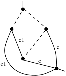
We draw the broken edges as dashed edges and the unbroken edges as solid edges having a color. As usual, as the fields are matrices, the order of the half edges around a vertex is relevant and the Feynman graphs are in fact combinatorial maps (a.k.a. ribbon graphs [1]). An example of a map with broken and unbroken edges is presented in Figure 4.

Refer to caption
Figure 4: Map with cilia, broken and unbroken colored edges.

In the perturbative Feynman expansion, the generating function writes as a sum over maps ℳ{\cal{M}} with ciliated vertices whose edges fall in two categories: the unbroken edges ℰu​(ℳ){\cal{E}}_{u}({\cal{M}}), which have a color cc, and the broken edges, ℰb​(ℳ){\cal{E}}_{b}({\cal{M}}). Let us denote σℳ\sigma_{{\cal{M}}} the successor permutation of the map ℳ{\cal{M}}, and let us denote the corner (h,σℳ​(h))\big(h,\sigma_{{\cal{M}}}(h)\big) by [h][h]. Estimating the derivatives acting on the vertices, we obtain for every corner of the map an associated matrix element of an operator:

  • •

    for any corner [h][h] of a ciliated vertex or of a non ciliated vertex of coordination at least three we obtain:

    b​[1𝟏𝒟−b​M]a[h]𝒟​b[h]𝒟,b\left[\frac{1}{\mathbf{1}^{{\cal{D}}}-bM}\right]_{a^{{\cal{D}}}_{[h]}b^{{\cal{D}}}_{[h]}}\;,
  • •

    for a corner [h][h] of a non ciliated vertex of coordination one we obtain:

    b​[1𝟏𝒟−b​M−ab​𝟏𝒟−b​M]a[h]𝒟​b[h]𝒟,b\left[\frac{1}{\mathbf{1}^{{\cal{D}}}-bM}-\frac{a}{b}\mathbf{1}^{{\cal{D}}}-bM\right]_{a^{{\cal{D}}}_{[h]}b^{{\cal{D}}}_{[h]}}\;,
  • •

    for the couple of corners [h][h] and [σℳ​(h)][\sigma_{{\cal{M}}}(h)] belonging to a non ciliated vertex of coordination two we obtain:

    b2​([1𝟏𝒟−b​M]a[h]𝒟​b[h]𝒟​[1𝟏𝒟−b​M]a[σ⁡(h)]𝒟​b[σ⁡(h)]𝒟−[𝟏𝒟]a[h]𝒟​b[h]𝒟​[𝟏𝒟]a[σ⁡(h)]𝒟​b[σ⁡(h)]𝒟).\displaystyle b^{2}\Big(\left[\frac{1}{\mathbf{1}^{{\cal{D}}}-bM}\right]_{a^{{\cal{D}}}_{[h]}b^{{\cal{D}}}_{[h]}}\left[\frac{1}{\mathbf{1}^{{\cal{D}}}-bM}\right]_{a_{[\sigma(h)]}^{{\cal{D}}}b_{[\sigma(h)]}^{{\cal{D}}}}-[{\bf 1}^{{\cal{D}}}]_{a^{{\cal{D}}}_{[h]}b^{{\cal{D}}}_{[h]}}[{\bf 1}^{{\cal{D}}}]_{a_{[\sigma(h)]}^{{\cal{D}}}b_{[\sigma(h)]}^{{\cal{D}}}}\Big)\;.

The edges contract the indices of the operators incident at their ends in a specific pattern, according to the nature of the edge (unbroken or broken). Extracting the logarithm we obtain a sum over connected maps. We denote nint​(ℳ)n_{\rm int}({\cal{M}}), next​(ℳ)n_{\rm ext}({\cal{M}}), Eu​(ℳ)E_{u}({\cal{M}}) and Eb​(ℳ)E_{b}({\cal{M}}) the numbers of internal vertices, external vertices, unbroken edges and broken edges of ℳ{\cal{M}}. Recall that 𝒮⁡(ℳ){\cal S}({\cal{M}}) denotes the set of all the halfedges of ℳ{\cal{M}}, and 𝒮ext​(ℳ){\cal S}_{\rm ext}({\cal{M}}) the set of cilia of ℳ{\cal{M}}. With thees notations, the perturbative expansion of the generating function of the cumulants writes as:

ln⁡Z(4)​(J,J¯)=−ND​(D​a22+ln⁡(1−g​D​a))−D⁡(N2−1)2​ln⁡(1−b2)−12​ln⁡(1−D​b2)+\displaystyle\ln Z^{(4)}(J,\bar{J})=-N^{D}\left(\frac{Da^{2}}{2}+\ln(1-gDa)\right)-\frac{D(N^{2}-1)}{2}\ln(1-b^{2})-\frac{1}{2}\ln(1-Db^{2})+
+∑ℳ​connectedb2​Eu​(ℳ)+2​Eb​(ℳ)nint​(ℳ)!​next​(ℳ)!∑a​b[(∏h∈𝒮⁡(ℳ)ℜ(M)a[h]𝒟​b[h]𝒟)(∏h∈𝒮ext​(ℳ)Ja[h]𝒟​J¯b[σℳ−1​(h)]𝒟ND−1​(1−g​D​a))\displaystyle+\sum_{{\cal{M}}\;{\rm connected}}\frac{b^{2E_{u}({\cal{M}})+2E_{b}({\cal{M}})}}{n_{\rm int}({\cal{M}})!n_{\rm ext}({\cal{M}})!}\sum_{ab}\Bigg[\left(\prod_{h\in{\cal S}({\cal{M}})}\mathfrak{R}(M)_{a^{{\cal{D}}}_{[h]}b^{{\cal{D}}}_{[h]}}\right)\left(\prod_{h\in{\cal S}_{\rm ext}({\cal{M}})}\frac{J_{a^{{\cal{D}}}_{[h]}}\bar{J}_{b^{{\cal{D}}}_{[\sigma_{{\cal{M}}}^{-1}(h)]}}}{N^{D-1}(1-gDa)}\right)
×[∏ec=(h,h′)∈ℰu​(ℳ)1ND−1​(1−b2)​(δb[σℳ−1​(h)]c​a[h′]c​δb[σℳ−1​(h′)]c​a[h]c)​(δb[σℳ−1​(h)]𝒟∖{c}​a[h]𝒟∖{c}​δb[σℳ−1​(h′)]𝒟∖{c}​a[h′]𝒟∖{c})]\displaystyle\;\;\times\Big[\prod_{e^{c}=(h,h^{\prime})\in{\cal{E}}_{u}({\cal{M}})}\frac{1}{N^{D-1}(1-b^{2})}\left(\delta_{b^{c}_{[\sigma_{{\cal{M}}}^{-1}(h)]}a^{c}_{[h^{\prime}]}}\delta_{b^{c}_{[\sigma_{{\cal{M}}}^{-1}(h^{\prime})]}a^{c}_{[h]}}\right)\left(\delta_{b^{{\cal{D}}\setminus\{c\}}_{[\sigma_{{\cal{M}}}^{-1}(h)]}a^{{\cal{D}}\setminus\{c\}}_{[h]}}\delta_{b^{{\cal{D}}\setminus\{c\}}_{[\sigma_{{\cal{M}}}^{-1}(h^{\prime})]}a^{{\cal{D}}\setminus\{c\}}_{[h^{\prime}]}}\right)\Big]
×[∏e=(h,h′)∈ℰb​(ℳ)b2​D​(D−1)ND​(1−b2)​(1−D​b2)(δb[σℳ−1​(h)]𝒟​a[h]𝒟δb[σℳ−1​(h′)]𝒟​a[h′]𝒟)]]M=0,\displaystyle\;\;\times\Big[\prod_{e=(h,h^{\prime})\in{\cal{E}}_{b}({\cal{M}})}\frac{b^{2}D(D-1)}{N^{D}(1-b^{2})(1-Db^{2})}\left(\delta_{b^{{\cal{D}}}_{[\sigma_{{\cal{M}}}^{-1}(h)]}a^{{\cal{D}}}_{[h]}}\delta_{b^{{\cal{D}}}_{[\sigma_{{\cal{M}}}^{-1}(h^{\prime})]}a^{{\cal{D}}}_{[h^{\prime}]}}\right)\Big]\Bigg]_{M=0}\;,

where we have used the notation:

  • •

    for any corner [h][h] of a ciliated vertex or of a non ciliated vertex of coordination at least three:

    ℜ​(M)a[h]𝒟​b[h]𝒟≡[1𝟏𝒟−b​M]a[h]𝒟​b[h]𝒟,\mathfrak{R}(M)_{a^{{\cal{D}}}_{[h]}b^{{\cal{D}}}_{[h]}}\equiv\left[\frac{1}{\mathbf{1}^{{\cal{D}}}-bM}\right]_{a^{{\cal{D}}}_{[h]}b^{{\cal{D}}}_{[h]}}\;,
  • •

    for a corner [h][h] of a non ciliated vertex of coordination one:

    ℜ​(M)a[h]𝒟​b[h]𝒟≡[1𝟏𝒟−b​M−ab​𝟏𝒟−b​M]a[h]𝒟​b[h]𝒟,\mathfrak{R}(M)_{a^{{\cal{D}}}_{[h]}b^{{\cal{D}}}_{[h]}}\equiv\left[\frac{1}{\mathbf{1}^{{\cal{D}}}-bM}-\frac{a}{b}\mathbf{1}^{{\cal{D}}}-bM\right]_{a^{{\cal{D}}}_{[h]}b^{{\cal{D}}}_{[h]}}\;,
  • •

    for the couple of corners [h][h] and [σℳ​(h)][\sigma_{{\cal{M}}}(h)] belonging to a non ciliated vertex of coordination two:

    ℜ​(M)a[h]𝒟​b[h]𝒟​ℜ​(M)a[σ⁡(h)]𝒟​b[σ⁡(h)]𝒟≡[1𝟏𝒟−b​M]a[h]𝒟​b[h]𝒟​[1𝟏𝒟−b​M]a[σ⁡(h)]𝒟​b[σ⁡(h)]𝒟−[𝟏𝒟]a[h]𝒟​b[h]𝒟​[𝟏𝒟]a[σ⁡(h)]𝒟​b[σ⁡(h)]𝒟.\displaystyle\mathfrak{R}(M)_{a^{{\cal{D}}}_{[h]}b^{{\cal{D}}}_{[h]}}\mathfrak{R}(M)_{a^{{\cal{D}}}_{[\sigma(h)]}b^{{\cal{D}}}_{[\sigma(h)]}}\equiv\left[\frac{1}{\mathbf{1}^{{\cal{D}}}-bM}\right]_{a^{{\cal{D}}}_{[h]}b^{{\cal{D}}}_{[h]}}\left[\frac{1}{\mathbf{1}^{{\cal{D}}}-bM}\right]_{a_{[\sigma(h)]}^{{\cal{D}}}b_{[\sigma(h)]}^{{\cal{D}}}}-[{\bf 1}^{{\cal{D}}}]_{a^{{\cal{D}}}_{[h]}b^{{\cal{D}}}_{[h]}}[{\bf 1}^{{\cal{D}}}]_{a_{[\sigma(h)]}^{{\cal{D}}}b_{[\sigma(h)]}^{{\cal{D}}}}\;.

7 Translating to the melonic vacuum

If we translate to the melonic vacuum, several significant simplifications can be made. Using b⁡(a0)=a0b(a_{0})=a_{0} and taking into account that MM is set to zero we obtain:

  • •

    for any corner [h][h] of a ciliated vertex or of a non ciliated vertex of coordination at least three:

    ℜ​(0)a[h]𝒟​b[h]𝒟=𝟏a[h]𝒟​b[h]𝒟𝒟,\mathfrak{R}(0)_{a^{{\cal{D}}}_{[h]}b^{{\cal{D}}}_{[h]}}=\mathbf{1}^{{\cal{D}}}_{a^{{\cal{D}}}_{[h]}b^{{\cal{D}}}_{[h]}}\;,
  • •

    for a corner [h][h] of a non ciliated vertex of coordination one:

    ℜ​(0)a[h]𝒟​b[h]𝒟=b⁡(a0)−a0b⁡(a0)​𝟏a[h]𝒟​b[h]𝒟𝒟=0,\mathfrak{R}(0)_{a^{{\cal{D}}}_{[h]}b^{{\cal{D}}}_{[h]}}=\frac{b(a_{0})-a_{0}}{b(a_{0})}\mathbf{1}^{{\cal{D}}}_{a^{{\cal{D}}}_{[h]}b^{{\cal{D}}}_{[h]}}=0\;,
  • •

    for the couple of corners [h][h] and [σℳ​(h)][\sigma_{{\cal{M}}}(h)] belonging to a non ciliated vertex of coordination two:

    ℜ​(0)a[h]𝒟​b[h]𝒟​ℜ​(0)a[σ⁡(h)]𝒟​b[σ⁡(h)]𝒟\displaystyle\mathfrak{R}(0)_{a^{{\cal{D}}}_{[h]}b^{{\cal{D}}}_{[h]}}\mathfrak{R}(0)_{a^{{\cal{D}}}_{[\sigma(h)]}b^{{\cal{D}}}_{[\sigma(h)]}}
    =[𝟏𝒟]a[h]𝒟​b[h]𝒟​[𝟏𝒟]a[σ⁡(h)]𝒟​b[σ⁡(h)]𝒟−[𝟏𝒟]a[h]𝒟​b[h]𝒟​[𝟏𝒟]a[σ⁡(h)]𝒟​b[σ⁡(h)]𝒟=0.\displaystyle\quad=[{\bf 1}^{{\cal{D}}}]_{a^{{\cal{D}}}_{[h]}b^{{\cal{D}}}_{[h]}}[{\bf 1}^{{\cal{D}}}]_{a_{[\sigma(h)]}^{{\cal{D}}}b_{[\sigma(h)]}^{{\cal{D}}}}-[{\bf 1}^{{\cal{D}}}]_{a^{{\cal{D}}}_{[h]}b^{{\cal{D}}}_{[h]}}[{\bf 1}^{{\cal{D}}}]_{a_{[\sigma(h)]}^{{\cal{D}}}b_{[\sigma(h)]}^{{\cal{D}}}}=0\;.

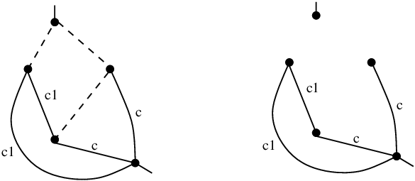
Thus only maps whose internal vertices have coordination at least three (which we denote ℳ3{\cal{M}}^{3}) survive. Moreover, a map ℳ3{\cal{M}}^{3} has unbroken colored edges and broken edges. Erasing all the broken edges leads to a map whose edges are colored by a color c={1,…​D}c=\{1,\dots D\}. We denote this map by ℳu3{\cal{M}}^{3}_{u} (as it is formed only by the unbroken edges). Remark that ℳu3{\cal{M}}^{3}_{u} can be disconnected, even though ℳ3{\cal{M}}^{3} is connected (see Figure 5).

Refer to caption
Figure 5: The maps ℳ3{\cal{M}}^{3} and ℳu3{\cal{M}}^{3}_{u}.

As ℳu3{\cal{M}}^{3}_{u} is a usual edge colored map it has a well defined notion of boundary graph ∂ℳu3\partial{\cal{M}}^{3}_{u} and (internal and external) faces. The indices are identified along the faces of ℳu3{\cal{M}}^{3}_{u}. As the numbers of unbroken edges of ℳ3{\cal{M}}^{3} and ℳu3{\cal{M}}^{3}_{u} are equal, and the number of ciliated vertices of ℳ{\cal{M}} is the number of white vertices of ∂ℳu3\partial{\cal{M}}^{3}_{u} we obtain:

ln⁡Z(4)​(J,J¯)=\displaystyle\ln Z^{(4)}(J,\bar{J})= −ND​(D​a22+ln⁡(1−g​D​a))−D⁡(N2−1)2​ln⁡(1−b2)−12​ln⁡(1−D​b2)+\displaystyle-N^{D}\left(\frac{Da^{2}}{2}+\ln(1-gDa)\right)-\frac{D(N^{2}-1)}{2}\ln(1-b^{2})-\frac{1}{2}\ln(1-Db^{2})+
+∑ℳ3​connectedTr∂ℳu3⁡(J,J¯)k⁡(∂ℳu3)!1nint​(ℳ3)!\displaystyle+\sum_{{\cal{M}}^{3}\;{\rm connected}}\frac{\Tr_{\partial{\cal{M}}^{3}_{u}}(J,\bar{J})}{k(\partial{\cal{M}}^{3}_{u})!}\frac{1}{n_{\rm int}({\cal{M}}^{3})!}
×a02​Eu​(ℳ3)+2​Eb​(ℳ3)(1−g​D​a0)k⁡(∂ℳu3)​[11−a02]Eu​(ℳ3)​[a02​D​(D−1)(1−a02)​(1−D​a02)]Eb​(ℳ3)\displaystyle\qquad\qquad\times\frac{a_{0}^{2E_{u}({\cal{M}}^{3})+2E_{b}({\cal{M}}^{3})}}{(1-gDa_{0})^{k(\partial{\cal{M}}^{3}_{u})}}\left[\frac{1}{1-a_{0}^{2}}\right]^{E_{u}({\cal{M}}^{3})}\left[\frac{a_{0}^{2}D(D-1)}{(1-a_{0}^{2})(1-Da_{0}^{2})}\right]^{E_{b}({\cal{M}}^{3})}
×N−D​Eb​(ℳ3)−(D−1)​Eu​(ℳ3)−(D−1)​k​(∂ℳu3)+Fint​(ℳu3),\displaystyle\qquad\qquad\times N^{-DE_{b}({\cal{M}}^{3})-(D-1)E_{u}({\cal{M}}^{3})-(D-1)k(\partial{\cal{M}}^{3}_{u})+F_{\rm int}({\cal{M}}^{3}_{u})}\;,

where k⁡(∂ℳu3)k(\partial{\cal{M}}^{3}_{u}) denotes the number of white vertices of the boundary graph ∂ℳu3\partial{\cal{M}}^{3}_{u} (see definition 8) and

Tr∂ℳu3⁡(J,J¯)=∏i=1k⁡(∂ℳu3)J¯a¯i𝒟​Jai𝒟​∏ec=(vi,v¯j)∈ℰ⁡(ℳu3)δaic​a¯jc.\Tr_{\partial{\cal{M}}^{3}_{u}}(J,\bar{J})=\prod_{i=1}^{k(\partial{\cal{M}}^{3}_{u})}\bar{J}_{\bar{a}^{{\cal{D}}}_{i}}J_{a^{{\cal{D}}}_{i}}\prod_{e^{c}=(v_{i},\bar{v}_{j})\in{\cal{E}}({\cal{M}}^{3}_{u})}\delta_{a^{c}_{i}\bar{a}^{c}_{j}}\;.

The rescaled cumulants are computed by taking derivatives and dividing by the appropriate power of NN:

K⁡(ℬ,μ(4))\displaystyle K({\cal{B}},\mu^{(4)}) =∑ℳ3​connected∂ℳu3=ℬ1nint​(ℳ3)!​a02​Eu​(ℳ3)+4​Eb​(ℳ3)(1−g​D​a0)k⁡(∂ℳu3)​[D⁡(D−1)]Eb​(ℳ3)(1−a02)Eu​(ℳ3)+Eb​(ℳ3)​(1−D​a02)Eb​(ℳ3)\displaystyle=\sum_{\genfrac{}{}{0.0pt}{}{\cM^3 \; {\rm connected}}{\partial\cM^3_u = \cB}}\frac{1}{n_{\rm int}({\cal{M}}^{3})!}\frac{a_{0}^{2E_{u}({\cal{M}}^{3})+4E_{b}({\cal{M}}^{3})}}{(1-gDa_{0})^{k(\partial{\cal{M}}^{3}_{u})}}\frac{[D(D-1)]^{E_{b}({\cal{M}}^{3})}}{(1-a_{0}^{2})^{E_{u}({\cal{M}}^{3})+E_{b}({\cal{M}}^{3})}(1-Da_{0}^{2})^{E_{b}({\cal{M}}^{3})}} (14)
×N−D​Eb​(ℳ3)−(D−1)​Eu​(ℳ3)−D+(D−1)​k​(∂ℳu3)+C⁡(∂ℳu3)+Fint​(ℳu3).\displaystyle\qquad\qquad\times N^{-DE_{b}({\cal{M}}^{3})-(D-1)E_{u}({\cal{M}}^{3})-D+(D-1)k(\partial{\cal{M}}^{3}_{u})+C(\partial{\cal{M}}^{3}_{u})+F_{\rm int}({\cal{M}}^{3}_{u})}\;. (15)

7.1 The 1/N1/N expansion for the fluctuation field

In this section we show that the cumulants admit a 1/N1/N expansion. We label ℳu;(ρ)3{\cal{M}}^{3}_{u;(\rho)} the connected components of ℳu3{\cal{M}}^{3}_{u} and we denote C⁡(ℳu3)C({\cal{M}}^{3}_{u}) their number.

Definition 9.

For each connected component ℳu;(ρ)3{\cal{M}}^{3}_{u;(\rho)} we define its deficit η⁡(ℳu;(ρ)3)\eta({\cal{M}}^{3}_{u;(\rho)}) as:

η⁡(ℳu;(ρ)3)=2+Eu​(ℳu;(ρ)3)+(D−2)​V​(ℳu;(ρ)3)−\displaystyle\eta({\cal{M}}^{3}_{u;(\rho)})=2+E_{u}({\cal{M}}^{3}_{u;(\rho)})+(D-2)V({\cal{M}}^{3}_{u;(\rho)})-
−(D−1)​k​(∂ℳu;(ρ)3)−C⁡(∂ℳu;(ρ)3)−Fint​(ℳu;(ρ)3).\displaystyle\qquad\qquad\qquad-(D-1)k(\partial{\cal{M}}^{3}_{u;(\rho)})-C(\partial{\cal{M}}^{3}_{u;(\rho)})-F_{\rm int}({\cal{M}}^{3}_{u;(\rho)})\;.

Furthermore, we define the excess of broken edges of ℳ3{\cal{M}}^{3}, Lb​(ℳ3)L_{b}({\cal{M}}^{3}), and the excess of unbroken edges of ℳu;(ρ)3{\cal{M}}^{3}_{u;(\rho)}, Lu​(ℳu;(ρ)3)L_{u}({\cal{M}}^{3}_{u;(\rho)}), as:

Lb​(ℳ3)≡Eb​(ℳ3)−C⁡(ℳu3)+1,Lu​(ℳu;(ρ)3)≡Eu​(ℳu;(ρ)3)−V⁡(ℳu;(ρ)3)+1.L_{b}({\cal{M}}^{3})\equiv E_{b}({\cal{M}}^{3})-C({\cal{M}}_{u}^{3})+1\;,\;\;L_{u}({\cal{M}}^{3}_{u;(\rho)})\equiv E_{u}({\cal{M}}^{3}_{u;(\rho)})-V({\cal{M}}^{3}_{u;(\rho)})+1\;.
Theorem 1 (1/N1/N expansion).

The rescaled cumulants of μ(4)\mu^{(4)} can be expressed as the formal series:

K⁡(ℬ,μ(4))=\displaystyle K({\cal{B}},\mu^{(4)})= ∑ℳ3​connected∂ℳu3=ℬ1nint​(ℳ3)!​a02​Eu​(ℳ3)+4​Eb​(ℳ3)(1−g​D​a0)k⁡(∂ℳu3)​[D⁡(D−1)]Eb​(ℳ3)(1−a02)Eu​(ℳ3)+Eb​(ℳ3)​(1−D​a02)Eb​(ℳ3)\displaystyle\sum_{\genfrac{}{}{0.0pt}{}{\cM^3 \; {\rm connected}}{\partial\cM^3_u = \cB}}\frac{1}{n_{\rm int}({\cal{M}}^{3})!}\frac{a_{0}^{2E_{u}({\cal{M}}^{3})+4E_{b}({\cal{M}}^{3})}}{(1-gDa_{0})^{k(\partial{\cal{M}}^{3}_{u})}}\frac{[D(D-1)]^{E_{b}({\cal{M}}^{3})}}{(1-a_{0}^{2})^{E_{u}({\cal{M}}^{3})+E_{b}({\cal{M}}^{3})}(1-Da_{0}^{2})^{E_{b}({\cal{M}}^{3})}} (16)
×N−D​Lb​(ℳ3)−(D−2)​∑ρ=1C⁡(ℳu3)Lu​(ℳu;(ρ)3)−∑ρ=1C⁡(ℳu3)η⁡(ℳu;(ρ)3).\displaystyle\qquad\qquad\times N^{-DL_{b}({\cal{M}}^{3})-(D-2)\sum_{\rho=1}^{C({\cal{M}}^{3}_{u})}L_{u}({\cal{M}}^{3}_{u;(\rho)})-\sum_{\rho=1}^{C({\cal{M}}^{3}_{u})}\eta({\cal{M}}^{3}_{u;(\rho)})}\;. (17)

The right hand side of Eq. (16) is a series in 1/N1/N. More importantly, there are only a finite number of maps ℳ3{\cal{M}}^{3} contributing to any fixed order in 1/N1/N.

Proof.

A straightforward computation leads from Eq. (14) to Eq. (16) taking into account that the boundary graph and the internal faces of ℳu3{\cal{M}}_{u}^{3} are distributed among the connected components ℳu;(ρ)3{\cal{M}}^{3}_{u;(\rho)} and that the numbers of vertices, ciliated vertices and unbroken edges of ℳ3{\cal{M}}^{3} and ℳu3{\cal{M}}^{3}_{u} are equal.

As ℳ3{\cal{M}}^{3} is connected, all the connected components of ℳu3{\cal{M}}^{3}_{u} must be connected in between them by broken edges, hence Lb​(ℳ3)≥0L_{b}({\cal{M}}^{3})\geq 0. Similarly, as ℳu;(ρ)3{\cal{M}}^{3}_{u;(\rho)} is connected, Lu​(ℳu;(ρ)3)≥0L_{u}({\cal{M}}^{3}_{u;(\rho)})\geq 0.

In appendix A we prove the following lemma:

Lemma 2.

The number of internal faces of a connected edge colored map with k⁡(∂ℳ)k(\partial{\cal{M}}) cilia is bounded by:

Fint​(ℳ)\displaystyle F_{\rm int}({\cal{M}}) ≤1−(D−1)​k​(∂ℳ)−C⁡(∂ℳ)+(D−1)​V​(ℳ)+[E⁡(ℳ)−V⁡(ℳ)+1].\displaystyle\leq 1-(D-1)k(\partial{\cal{M}})-C(\partial{\cal{M}})+(D-1)V({\cal{M}})+[E({\cal{M}})-V({\cal{M}})+1]\;.

As a consequence of this lemma, for any connected component ℳu;(ρ)3{\cal{M}}^{3}_{u;(\rho)}, its deficit η⁡(ℳu;(ρ)3)\eta({\cal{M}}^{3}_{u;(\rho)}) is non negative, η⁡(ℳu;(ρ)3)≥0\eta({\cal{M}}^{3}_{u;(\rho)})\geq 0. It follows that the right hand side of Eq. (16) is a series in 1/N1/N.

In order to prove the second part of the theorem, we note that, as D>D−2D>D-2, the scaling in NN is bounded by:

−(D−2)​[Lb​(ℳ3)+∑ρ=1C⁡(ℳu3)Lu​(ℳu;(ρ)3)]=−(D−2)​[Eb​(ℳ3)+Eu​(ℳ3)−V⁡(ℳ3)+1].\displaystyle-(D-2)\Big[L_{b}({\cal{M}}^{3})+\sum_{\rho=1}^{C({\cal{M}}^{3}_{u})}L_{u}({\cal{M}}^{3}_{u;(\rho)})\Big]=-(D-2)\big[E_{b}({\cal{M}}^{3})+E_{u}({\cal{M}}^{3})-V({\cal{M}}^{3})+1\big]\;.

As the ciliated vertices in the map ℳ3{\cal{M}}^{3} have coordination at least one, while the non ciliated vertices have coordination at least three, we have:

2​[Eb​(ℳ3)+Eu​(ℳ3)]≥3​[V⁡(ℳ3)−k⁡(∂ℳu3)]+k⁡(∂ℳu3)⇒V⁡(ℳ3)≤23​[Eb​(ℳ3)+Eu​(ℳ3)+k⁡(∂ℳu3)],\displaystyle 2\big[E_{b}({\cal{M}}^{3})+E_{u}({\cal{M}}^{3})\big]\geq 3\left[V({\cal{M}}^{3})-k(\partial{\cal{M}}^{3}_{u})\right]+k(\partial{\cal{M}}^{3}_{u})\Rightarrow V({\cal{M}}^{3})\leq\frac{2}{3}\big[E_{b}({\cal{M}}^{3})+E_{u}({\cal{M}}^{3})+k(\partial{\cal{M}}^{3}_{u})\big]\;,

hence the scaling with NN of a term on the right hand side of Eq. (14) is bounded by:

−(D−2)​[Eb​(ℳ3)+Eu​(ℳ3)3−2​k​(∂ℳu3)3+1].-(D-2)\left[\frac{E_{b}({\cal{M}}^{3})+E_{u}({\cal{M}}^{3})}{3}-\frac{2k(\partial{\cal{M}}^{3}_{u})}{3}+1\right]\;.

The number of external vertices of ℳu3{\cal{M}}^{3}_{u} is fixed, as it equals the number of the white vertices of the invariant ℬ{\cal{B}} whose cumulant we evaluate. It follows that at any order in 1/N1/N only connected maps with at most a finite number of edges contribute, and the second part of the theorem follows.

∎

Setting the external sources to zero we obtain the free energy of the quartic melonic model:

ln⁡Z(4)=\displaystyle\ln Z^{(4)}= −ND​(D​a22+ln⁡(1−g​D​a))−D⁡(N2−1)2​ln⁡(1−b2)−12​ln⁡(1−D​b2)+\displaystyle-N^{D}\left(\frac{Da^{2}}{2}+\ln(1-gDa)\right)-\frac{D(N^{2}-1)}{2}\ln(1-b^{2})-\frac{1}{2}\ln(1-Db^{2})+
+ND∑ℳ3​connected∂ℳ3=∅1nint​(ℳ3)!\displaystyle+N^{D}\sum_{\genfrac{}{}{0.0pt}{}{ \cM^3 \; {\rm connected} }{ \partial\cM^3 = \emptyset}}\frac{1}{n_{\rm int}({\cal{M}}^{3})!}
×a02​Eu​(ℳ3)+2​Eb​(ℳ3)​[11−a02]Eu​(ℳ3)​[a02​D​(D−1)(1−a02)​(1−D​a02)]Eb​(ℳ3)\displaystyle\qquad\qquad\times a_{0}^{2E_{u}({\cal{M}}^{3})+2E_{b}({\cal{M}}^{3})}\left[\frac{1}{1-a_{0}^{2}}\right]^{E_{u}({\cal{M}}^{3})}\left[\frac{a_{0}^{2}D(D-1)}{(1-a_{0}^{2})(1-Da_{0}^{2})}\right]^{E_{b}({\cal{M}}^{3})}
×N−D​Lb​(ℳ3)−(D−2)​∑ρ=1C⁡(ℳu3)Lu​(ℳu;(ρ)3)−∑ρ=1C⁡(ℳu3)η⁡(ℳu;(ρ)3).\displaystyle\qquad\qquad\times N^{-DL_{b}({\cal{M}}^{3})-(D-2)\sum_{\rho=1}^{C({\cal{M}}^{3}_{u})}L_{u}({\cal{M}}^{3}_{u;(\rho)})-\sum_{\rho=1}^{C({\cal{M}}^{3}_{u})}\eta({\cal{M}}^{3}_{u;(\rho)})}\;.

The sum over ℳ3{\cal{M}}^{3} does not contribute at leading oder in NN. Indeed, a term in the sum with Lb​(ℳ3)=Lu​(ℳu;(ρ)3)=0L_{b}({\cal{M}}^{3})=L_{u}({\cal{M}}^{3}_{u;(\rho)})=0 would be a tree, hence would have univalent vertices, which is impossible as all the vertices ℳ3{\cal{M}}^{3} are at least three valent.

Appendix A Proof of lemma 2

In this appendix we show that the number of internal faces of a connected edge colored map ℳ{\cal{M}} cilia is bounded by:

Fint​(ℳ)\displaystyle F_{\rm int}({\cal{M}}) ≤1−(D−1)​k​(∂ℳ)−C⁡(∂ℳ)+(D−1)​V​(ℳ)+[E⁡(ℳ)−V⁡(ℳ)+1].\displaystyle\leq 1-(D-1)k(\partial{\cal{M}})-C(\partial{\cal{M}})+(D-1)V({\cal{M}})+[E({\cal{M}})-V({\cal{M}})+1]\;.
Proof.

In order to establish this bound, we first introduce a new colored map ℳ∗{\cal{M}}^{*} associated to ℳ{\cal{M}} which will allow us to keep track of the boundary ∂ℳ\partial{\cal{M}} while modifying ℳ{\cal{M}}. Starting from ℳ{\cal{M}}, for each cilium hh, we introduce 2​D2D half edges on the corner bearing the cilium hh, one at its left and one at its right for each color c∈𝒟c\in{\cal{D}} (that is, for each color cc, one half edge precedes hh and the other succeeds hh when turning around the vertex). We then connect these new half edges into dashed edges following the edges of ∂ℳ\partial{\cal{M}}: if the external strand of color cc starting at the cilium hh ends at the cilium h′h^{\prime}, we connect the half edge of color cc following hh with the half edge of color cc preceding h′h^{\prime}. This construction is represented in figure 7.

Refer to caption
Figure 6: A map ℳ{\cal{M}} with two cilia. For simplicity, only the colors 1 and 2 have been represented.

Each of the external strands of ℳ{\cal{M}} corresponds to an edge in the boundary graph ∂ℳ\partial{\cal{M}}, hence ℳ{\cal{M}} has exactly D​k​(∂ℳ)Dk(\partial{\cal{M}}) external strands. By construction ℳ∗{\cal{M}}^{*} has a new edge for each external strand of ℳ{\cal{M}} which closes the external strand of ℳ{\cal{M}} into an internal face of ℳ∗{\cal{M}}^{*}. It follows that:

Fint​(ℳ∗)=Fint​(ℳ)+D​k​(∂ℳ).F_{\rm int}({\cal{M}}^{*})=F_{\rm int}({\cal{M}})+Dk(\partial{\cal{M}})\ .

On the other hand, as the new dashed edges exactly follow the external strands of ℳ{\cal{M}}, it ensues that ∂ℳ∗=∂ℳ\partial{\cal{M}}^{*}=\partial{\cal{M}}.

Refer to caption
Figure 7: The map ℳ∗{\cal{M}}^{*} obtained from the map ℳ{\cal{M}} in Fig. 6 by adding the dashed edges.

The reason to introduce ℳ∗{\cal{M}}^{*} is the following. Below we will delete solid edges of ℳ∗{\cal{M}}^{*} (that is edges which belonged to ℳ{\cal{M}}) and track the change in the number of internal faces of ℳ∗{\cal{M}}^{*} under these deletions. The crucial point is that these deletions modify the structure of the internal faces of ℳ∗{\cal{M}}^{*} but do not modify its external strands, hence the boundary graph ∂ℳ∗\partial{\cal{M}}^{*} will remain unchanged. The introduction of ℳ∗{\cal{M}}^{*} allows us to modify a map while keeping its boundary graph unchanged.

Let 𝒯{\cal{T}} be a tree in ℳ{\cal{M}} and let us denote 𝒯∗{\cal{T}}^{*} the graph made of 𝒯{\cal{T}} and all dashed edges of ℳ∗{\cal{M}}^{*}. We have:

∂𝒯∗=∂ℳ∗=∂ℳ.\partial{\cal{T}}^{*}=\partial{\cal{M}}^{*}=\partial{\cal{M}}\;.

The map 𝒯∗{\cal{T}}^{*} can be obtained from ℳ∗{\cal{M}}^{*} by deleting E⁡(ℳ)−V⁡(ℳ)+1E({\cal{M}})-V({\cal{M}})+1 solid edges. As there is only one face going trough any of the solid edges, the deletion of such an edge in ℳ∗{\cal{M}}^{*} can either increase of decrease the number of faces by one, hence:

Fint​(ℳ)+D​k​(∂ℳ)=Fint​(ℳ∗)≤Fint​(𝒯∗)+E⁡(ℳ)−V⁡(ℳ)+1.\displaystyle F_{\rm int}({\cal{M}})+Dk(\partial{\cal{M}})=F_{\rm int}({\cal{M}}^{*})\ \leq\ F_{\rm int}({\cal{T}}^{*})\,+\,E({\cal{M}})-V({\cal{M}})+1\ .

We call a leaf of 𝒯∗{\cal{T}}^{*} a vertex which becomes univalent when one erases all the dashed edges. A moments reflexion reveals that the leafs of 𝒯∗{\cal{T}}^{*} are the univalent vertices of 𝒯{\cal{T}}. In order to complete the proof of lemma 2, it is now enough to show that for any 𝒯∗{\cal{T}}^{*} we have:

Fint​(𝒯∗)+C⁡(∂𝒯∗)≤1+k⁡(∂𝒯∗)+(D−1)​V​(𝒯∗).\displaystyle F_{\rm int}({\cal{T}}^{*})+C(\partial{\cal{T}}^{*})\leq 1+k(\partial{\cal{T}}^{*})+(D-1)V({\cal{T}}^{*})\ .

This bound is obtained by tracking the evolution of Fint​(𝒯∗)+C⁡(∂𝒯∗)F_{\rm int}({\cal{T}}^{*})+C(\partial{\cal{T}}^{*}) under the iterative deletion of the leaves. This deletion is somewhat involved, as it can change the boundary graph.

We say that an external strand of 𝒯∗{\cal{T}}^{*} is looped at the cilium hh if it starts and ends at the cilium hh. On the boundary graph ∂𝒯∗\partial{\cal{T}}^{*}, this corresponds to an edge connecting the black and white vertices associated to hh. In figure 7 we can identify two looped external strands. Let us denote ℓ\ell a leaf of 𝒯∗{\cal{T}}^{*} and let us denote 𝒯^∗\hat{\cal{T}}^{*} the tree obtained from 𝒯∗{\cal{T}}^{*} after deleting ℓ\ell as follows.

Deleting a non ciliated leaf.

If ℓ\ell has no cilium, deleting it simply means deleting the vertex ℓ\ell and the edge connecting it to the rest of 𝒯∗{\cal{T}}^{*}. If the edge connecting ℓ\ell to the rest of 𝒯∗{\cal{T}}^{*} has color cc, the deletion of ℓ\ell erases all the faces of colors 𝒟∖{c}{\cal{D}}\setminus\{c\} running trough ℓ\ell. The boundary graph is unaltered by this deletion, therefore:

Fint​(𝒯∗)=Fint​(𝒯^∗)+(D−1),\displaystyle F_{\rm int}({\cal{T}}^{*})=F_{\rm int}(\hat{\cal{T}}^{*})+(D-1)\;, C⁡(∂𝒯∗)=C⁡(∂𝒯^∗)⇒\displaystyle\qquad C(\partial{\cal{T}}^{*})=C(\partial\hat{\cal{T}}^{*})\Rightarrow
Fint​(𝒯∗)+C⁡(∂𝒯∗)\displaystyle F_{\rm int}({\cal{T}}^{*})+C(\partial{\cal{T}}^{*}) =Fint​(𝒯^∗)+C⁡(∂𝒯^∗)+(D−1).\displaystyle=F_{\rm int}(\hat{\cal{T}}^{*})+C(\partial\hat{\cal{T}}^{*})+(D-1)\ .
Deleting a ciliated leaf.

If ℓ\ell has a cilium hh, deleting it consists in :

  • •

    Step 1. For all the external strands starting or ending at hh that are not looped, we cut the corresponding dashed edges into half edges. We then reconnect the dashed half edges into edges the other way around, respecting the colors. This is represented in figure 8 below. Observe that after performing this step, all the external strands going trough ℓ\ell are looped.

    Refer to caption
    Figure 8: The first step of the deletion of a ciliated leaf : the dashed edges have been reconnected in such way that all the external strands are looped at the cilium hh.
  • •

    Step 2. The leaf now has only looped external strands and it is connected to the rest of the 𝒯∗{\cal{T}}^{*} by a solid edge only. The cilium hh represents a connected component of the boundary graph consisting in a black and a white vertex connected by DD edges. We erase the vertex ℓ\ell, its cilium, hh, and the edge connecting ℓ\ell to the rest of the graph, as in figure 9

    Refer to caption
    Figure 9: The second step of the deletion of a ciliated leaf.

Boundary graph. Upon deleting a ciliated leaf, the boundary graph changes: ∂𝒯^∗≠∂𝒯∗\partial\hat{\cal{T}}^{*}\neq\partial{\cal{T}}^{*}. We have two cases, each with two sub cases:

  • •

    None of the external strands of 𝒯∗{\cal{T}}^{*} are looped at hh. One needs to apply Step 1 for all the colors and then Step 2. There are two sub cases:

    • –

      the black and white vertices associated to hh in ∂𝒯∗\partial{\cal{T}}^{*} belong to the same connected component of ∂𝒯∗\partial{\cal{T}}^{*}. Then, in the boundary graph, Step 1 creates at least a new connected component, and Step 2 deletes exactly one connected component. Thus:

      C⁡(∂𝒯∗)≤C⁡(∂𝒯^∗).C(\partial{\cal{T}}^{*})\leq C(\partial\hat{\cal{T}}^{*})\;.
    • –

      the black and white vertices associated to hh in ∂𝒯∗\partial{\cal{T}}^{*} belong to different connected components of ∂𝒯∗\partial{\cal{T}}^{*}. Then, in the boundary graph, Step 1 can not decrease the number of connected components, and Step 2 deletes exactly one connected component. Thus:

      C⁡(∂𝒯∗)≤C⁡(∂𝒯^∗)+1.C(\partial{\cal{T}}^{*})\leq C(\partial\hat{\cal{T}}^{*})+1\;.
  • •

    At least one external strands of 𝒯∗{\cal{T}}^{*} is looped at hh. There are two sub cases:

    • –

      not all the external strands are looped at hh. The black and white vertices associated to hh in ∂𝒯∗\partial{\cal{T}}^{*} belong to the same connected component of ∂𝒯∗\partial{\cal{T}}^{*}. One must apply Step 1 at least once, and then step 2. As before, Step 1 creates at least a new connected component, and Step 2 deletes exactly one connected component, hence:

      C⁡(∂𝒯∗)≤C⁡(∂𝒯^∗).C(\partial{\cal{T}}^{*})\leq C(\partial\hat{\cal{T}}^{*})\;.
    • –

      all the external strands are looped at hh. The black and white vertices associated to hh in ∂𝒯∗\partial{\cal{T}}^{*} belong to two different connected components of ∂𝒯∗\partial{\cal{T}}^{*}, and one must apply Step 2 directly. This decrease the number of connect components of the boundary graph by 11:

      C⁡(∂𝒯∗)=C⁡(∂𝒯^∗)+1.C(\partial{\cal{T}}^{*})=C(\partial\hat{\cal{T}}^{*})+1\;.

Internal faces. Let us denote ece^{c} the solid edge of color cc connecting ℓ\ell to the rest of 𝒯∗{\cal{T}}^{*}. We have several cases:

  • •

    the external strand of color cc is looped at hh. Then there is only one internal face of color cc in 𝒯∗{\cal{T}}^{*} running through ece^{c}, which can not be erased by deleting ℓ\ell, hence:

    Fintc​(𝒯∗)=Fintc​(𝒯^∗).F_{\rm int}^{c}({\cal{T}}^{*})=F_{\rm int}^{c}(\hat{\cal{T}}^{*})\;.
  • •

    the external strand of color cc is not looped at hh. Then there are either one or two internal faces of color cc in 𝒯∗{\cal{T}}^{*} running trough ece^{c}, hence the number of internal faces of color cc can not decrease by more than one:

    Fintc​(𝒯∗)≤Fintc​(𝒯^∗)+1.F_{\rm int}^{c}({\cal{T}}^{*})\leq F_{\rm int}^{c}(\hat{\cal{T}}^{*})+1\;.
  • •

    the external strand of color c′≠cc^{\prime}\neq c is looped. Then there is only one internal face of color c′c^{\prime} through ℓ\ell, which is erased:

    Fintc′​(𝒯∗)=Fintc′​(𝒯^∗)+1.F_{\rm int}^{c^{\prime}}({\cal{T}}^{*})=F_{\rm int}^{c^{\prime}}(\hat{\cal{T}}^{*})+1\;.
  • •

    the external strand of color c′≠cc^{\prime}\neq c is not looped. Then there is just one internal face of color c′c^{\prime} through ℓ\ell, which is not erased:

    Fintc′​(𝒯∗)=Fintc′​(𝒯^∗).F_{\rm int}^{c^{\prime}}({\cal{T}}^{*})=F_{\rm int}^{c^{\prime}}(\hat{\cal{T}}^{*})\;.

Combining the counting of the connected components of the boundary graphs with the counting of the internal faces we obtain four cases:

  • •

    no external strand is looped at hh. Then:

    Fint​(𝒯∗)+C⁡(∂𝒯∗)≤[Fint​(𝒯^∗)+1]+[C⁡(∂𝒯^∗)+1]≤Fint​(𝒯^∗)+C⁡(∂𝒯^∗)+D.F_{\rm int}({\cal{T}}^{*})+C(\partial{\cal{T}}^{*})\leq[F_{\rm int}(\hat{\cal{T}}^{*})+1]+[C(\partial\hat{\cal{T}}^{*})+1]\leq F_{\rm int}(\hat{\cal{T}}^{*})+C(\partial\hat{\cal{T}}^{*})+D\;.
  • •

    all the external strands are looped at hh. Then:

    Fint​(𝒯∗)+C⁡(∂𝒯∗)≤[Fint​(𝒯^∗)+D−1]+[C⁡(∂𝒯^∗)+1]≤Fint​(𝒯^∗)+C⁡(∂𝒯^∗)+D.F_{\rm int}({\cal{T}}^{*})+C(\partial{\cal{T}}^{*})\leq[F_{\rm int}(\hat{\cal{T}}^{*})+D-1]+[C(\partial\hat{\cal{T}}^{*})+1]\leq F_{\rm int}(\hat{\cal{T}}^{*})+C(\partial\hat{\cal{T}}^{*})+D\;.
  • •

    the external strand of color cc is looped at hh, but at least one external strand of color c′≠cc^{\prime}\neq c is not looped at hh. Then:

    Fint​(𝒯∗)+C⁡(∂𝒯∗)≤[Fint​(𝒯^∗)+D−2]+[C⁡(∂𝒯^∗)]≤Fint​(𝒯^∗)+C⁡(∂𝒯^∗)+D.F_{\rm int}({\cal{T}}^{*})+C(\partial{\cal{T}}^{*})\leq[F_{\rm int}(\hat{\cal{T}}^{*})+D-2]+[C(\partial\hat{\cal{T}}^{*})]\leq F_{\rm int}(\hat{\cal{T}}^{*})+C(\partial\hat{\cal{T}}^{*})+D\;.
  • •

    the external strand of color cc is not looped at hh, but some external strands of colors c′≠cc^{\prime}\neq c are looped at hh. Then

    Fint​(𝒯∗)+C⁡(∂𝒯∗)≤[Fint​(𝒯^∗)+D]+[C⁡(∂𝒯^∗)]≤Fint​(𝒯^∗)+C⁡(∂𝒯^∗)+D.F_{\rm int}({\cal{T}}^{*})+C(\partial{\cal{T}}^{*})\leq[F_{\rm int}(\hat{\cal{T}}^{*})+D]+[C(\partial\hat{\cal{T}}^{*})]\leq F_{\rm int}(\hat{\cal{T}}^{*})+C(\partial\hat{\cal{T}}^{*})+D\;.

In all cases, by deleting a ciliated leaf:

Fintc​(𝒯∗)+C⁡(∂𝒯∗)≤Fintc​(𝒯^∗)+C⁡(∂𝒯^∗)+D.F_{\rm int}^{c}({\cal{T}}^{*})+C(\partial{\cal{T}}^{*})\leq F_{\rm int}^{c}(\hat{\cal{T}}^{*})+C(\partial\hat{\cal{T}}^{*})+D\;.

Iterating up to the last vertex, we either end up with a vertex with no cilium or with a ciliated vertex with DD looped external strands. Counting the number of internal faces and connected component of the two possible final graphs we conclude.

∎

References