Galilean Creation of the Inflationary Universe
Abstract
It has been pointed out that the null energy condition can be violated stably in some non-canonical scalar-field theories. This allows us to consider the Galilean Genesis scenario in which the universe starts expanding from Minkowski spacetime and hence is free from the initial singularity. We use this scenario to study the early-time completion of inflation, pushing forward the recent idea of Pirtskhalava et al. We present a generic form of the Lagrangian governing the background and perturbation dynamics in the Genesis phase, the subsequent inflationary phase, and the graceful exit from inflation, as opposed to employing the effective field theory approach. Our Lagrangian belongs to a more general class of scalar-tensor theories than the Horndeski theory and Gleyzes-Langlois-Piazza-Vernizzi generalization, but still has the same number of the propagating degrees of freedom, and thus can avoid Ostrogradski instabilities. We investigate the generation and evolution of primordial perturbations in this scenario and show that one can indeed construct a stable model of inflation preceded by (generalized) Galilean Genesis.
pacs
98.80.CqI Introduction
Inflation in the early Universe [1, 2] is now an indispensable ingredient of modern cosmology not only to explain the global properties of homogeneous and isotropic space with a vanishingly small spatial curvature but also to account for the origin of the primordial curvature perturbation that seeded cosmic structure formation [3]. At present, despite the significant progress in the state-of-the-art precise measurements of the cosmic microwave background radiation (CMB) by WMAP [4, 5] and Planck [6, 7] missions, there is no single observational result in conflict with the single-field inflation paradigm [2]. In particular, the anti-correlation of the temperature and the E-mode polarization anisotropies on large scales observed by the WMAP mission strongly supports the superhorizon perturbations suggested by inflation [8].
In other words, once inflation sets in, virtually all the available cosmological observation data can be explained simultaneously irrespective of the initial condition of the Universe. This does not mean that we may be indifferent to the initial condition of the Universe before inflation. On the contrary, in order to achieve complete understanding of the cosmic history, we must work out the very beginning of the Universe that may smoothly evolve into the inflationary phase.
As is well known, as long as the null energy condition (NEC) is satisfied in the expanding phase, the Hubble parameter and the energy density of the universe increase backward in cosmic time. So, it is often claimed that, if one tries to discuss what happened before inflation and/or how inflation started, one needs to know the information of very high energy physics, and challenge the initial singularity problem [9] in terms of quantum gravity. But, this is not always the case.
Recently, it was recognized that, if an action includes higher derivative terms of a scalar field like the Galileon terms, the NEC can be violated without encountering ghost nor gradient instabilities. See, e.g., Ref. [10] for a recent review and Ref. [11] for a subtle issue of nonlinear instabilities. If the NEC is violated, the energy density can grow as time proceeds, contrary to the conventional wisdom. In the NEC violating theories, the universe can therefore start from the static zero-energy state described by the Minkowski spacetime from infinite past [12], and the universe starts expansion with the increase of the energy density.
Such a picture of the emergence of the universe was first proposed by Creminelli et al. [13] with the name Galilean Genesis. In their model, however, the hot big bang state was postulated to be realized after the effective field theory description breaks down as the energy density blows up beyond its realm of validity. Therefore, the theory to describe the most important epoch of the early universe is lacking there.
Nevertheless, since their original idea is so interesting that a number of extension has been made in a wider class of scalar field theories [14, 15, 16, 17, 18] and various aspects of the Genesis scenario have been explored in the literature [19, 20, 21, 22, 23], such as avoidance of the superluminal propagation of perturbations and absence of primordial tensor perturbations. They have been unsuccessful, however, to realize transition from the Genesis phase to the hot big bang state within their model Lagrangians.
In this paper, we take a different approach, namely, to make use of the Galilean Genesis to explain the initial condition of the Universe before inflation and smoothly connect it to the inflationary phase, thereby solving the initial singularity problem [9] and the trans-Planckian problem [24] (see also [25]) in inflationary cosmology.
In fact, such an approach has also been put forward by Pirtskhalava et al. [26] recently. Their model Lagrangian, however, gives rise to gradient instability as it is, although it has been argued there that higher-order structure of the effective field theory for perturbations possesses enough freedom to cure the gradient instability. Discussion on termination of inflation and reheating is not presernted there, either.
In the present paper, we construct a specific model free from any catastrophic instabilities and with subluminal velocities of primordial perturbations. In our setup the universe starts from the Minkowski spacetime from infinite past and is smoothly connected to the inflationary phase followed by the graceful exit. For this purpose, we provide a generic Lagrangian capable of describing the background and perturbation evolution in all the above phases instead of choosing the effective field theory approach because the latter cannot capture the evolution of the background and perturbations from pre-inflationary Genesis to the exit from inflation with the same single Lagrangian.
Although we start with asymptotically Minkowski space at the past infinity for aesthetic beauty, it has been shown that the Galilean Genesis solution is an attractor for a variety of initial conditions including those with a negative Hubble parameter and/or finite curvature, provided that the time derivative of the scalar field has the right sign [18].
The Horndeski theory [27] or the generalized Galileon [28], whose mutual equivalence was first shown in [29], is known to be the most general scalar-tensor tensor theory with the second-order field equations, and thereby avoid Ostrogradski instabilities in spite of having higher derivative terms in the action. The theory can be generalized to have second-order field equations only in a specific gauge while maintaining the number of propagating degrees of freedom. This possibility was realized recently by Gleyzes et al. [30] (see also Ref. [31]) and was extended further by Gao [32]. The number of propagating degrees of freedom in these theories is indeed shown to be the same as that of the Horndeski theory [30, 32, 33, 34, 35, 36]. In this paper, we use the subclass of Gao’s framework as a concrete realization of the unified scenario starting from Galilean Genesis through inflation to the graceful exit.
This paper is organized as follows. In the next section, we give a framework of our model and derive the background equations of motion and the quadratic actions of cosmological perturbations. In Sec. III, a concrete Lagrangian is constructed to describe our scenario beginning from the Genesis phase through the inflationary one to the graceful exit, and such a background dynamics is presented explicitly. In Sec. IV, we discuss the stability during each phase based on the quadratic actions of cosmological perturbations. In Sec. V, a concrete realization of our scenario is given. The final section is devoted to our conclusions and discussion.
II General Framework
Let us start with describing the general framework to construct and study our explicit realization of the early-time completion of inflation. We would like to consider theories composed of a metric and a single scalar field , and hence it will be appropriate to work in the Horndeski theory. The Lagrangian of the Horndeski theory is of the form
| (1) | |||||
where , is the four-dimensional Ricci scalar, and is the four-dimensional Einstein tensor. We have four arbitrary functions of and in the Horndeski theory. This is the most general Lagrangian having second-order field equations. Nevertheless, it will turn out that this framework is insufficient for our purpose, and hence we have to go beyond the Horndeski theory.
One can generalize the Horndeski theory to possess higher order field equations while maintaining the number of propagating degrees of freedom [30]. The first step to do so is to perform an ADM decomposition by taking const hypersurfaces as constant time hypersurfaces. In the ADM language, the metric is written as
| (2) |
By definition is a function of only , , and , where a dot denotes differentiation with respect to , so any function of and can be regarded as a function of and the lapse function , provided that and never vanish. Then, the Horndeski Lagrangian (1) can be written in terms of the ADM variables as with
| (3) |
where and are the extrinsic and intrinsic curvature tensors on the constant time hypersurfaces, and , , , and are subject to the relations
| (4) |
Variation of the above Lagrangian with respect to gives a second-class constraint that eliminates only one degree of freedom, as opposed to general relativity. The key trick to generalize the Horndeski theory is to notice that this property remains the same even if one liberates and from the restriction imposed by Eq. (4) [30]. We thus arrive at the so called GLPV theory that is more general than Horndeski but has the same number of propagating degrees of freedom. One can move back to a covariant form of the Lagrangian by introducing the unit normal to the constant time hypersurfaces as , writing the extrinsic curvature tensor in terms of , and using the Gauss-Codazzi equations. Since there are six arbitrary functions of and in the ADM form, the resultant covariant Lagrangian has six arbitrary functions of and .
The above idea has been pushed forward by Gao [32], who proposed a unified framework to study single scalar-tensor theories beyond Horndeski. One can write a general Lagrangian in the ADM form as
| (5) | |||||
where the coefficients , , … are arbitrary functions of and . The Hamiltonian depends nonlinearly on as in the GLPV theory, giving rise to a single scalar degree of freedom on top of the traceless and transverse gravitons [35].
In this paper, we will employ the Lagrangian with
| (6) |
where , , and are constant parameters of the theory. This is a deformation of the GLPV Lagrangian and belongs to a subclass of Gao’s framework. The generalization to this level is sufficient for the purpose of the present paper. The GLPV theory is recovered by taking .
Given the Lagrangian (6) in the ADM form, one can restore the scalar degree of freedom to write its covariant expression in the same way as in the GLPV theory. However, it will be more convenient for our purpose to use the explicitly time-dependent Lagrangian, because by doing so one can easily design the Lagrangian so as to admit the desired cosmological evolution.
Before specifying the suitable form of , , … to construct our early universe model, let us derive the general equations governing the background and perturbation dynamics of cosmologies based on the Lagrangian (6). The ADM variables are given by
| (7) |
where is the curvature perturbation in the unitary gauge and is the transverse and traceless tensor perturbation. A spatially flat background has been assumed and the spatial diffeomorphism invariance was used to write in the above form. In the following, the background value of the lapse function is denoted by where there is no worry about confusion.
II.1 Background Equations
Substituting Eq. (7) to the Lagrangian (6), we obtain the background part of the Lagrangian as
| (8) |
where , , and . At the background level, , , and just rescale and . In what follows we simply consider the case with . Since we are considering a spatially flat universe, we have at zeroth order, and hence and play no role in the background dynamics. Varying Eq. (8) with respect to and , we obtain, respectively,
| (9) | |||||
| (10) | |||||
where a prime represents differentiation with respect to . The background equations contain at most second derivatives of the scale factor and first derivatives of the Lapse function.
II.2 Cosmological Perturbations
The quadratic Lagrangian for the tensor perturbation is given by
| (11) |
where
| (12) | |||||
| (13) |
The equation of motion contains at most second derivatives both in time and space. The tensor perturbation is stable provided that and .
The quadratic Lagrangian for the scalar perturbations is given by
| (14) | |||||
where the coefficients are defined as
| (15) | |||||
| (16) | |||||
| (17) | |||||
| (18) | |||||
| (19) |
and note the relation . One has in the Horndeski and GLPV theories, in which . Therefore, the last term in the Lagrangian (14) is the novel consequence of theories beyond GLPV.
From and we obtain
| (20) | |||||
| (21) |
Substituting Eqs. (20) and (21) into Eq. (14), we obtain the reduced Lagrangian for the curvature perturbation,
| (22) |
where
| (23) | |||||
| (24) | |||||
| (25) |
Thus, if , the equation of motion for has the fourth derivative in space, giving the dispersion relation
| (26) |
We require that in order to avoid ghost instabilities. However, we allow for a negative sound speed squared, , for a short period of time. In the absence of the term (), a negative sound speed squared would cause a rapid growth of instabilities for large modes. In this paper, we consider theories with , so that the curvature perturbation with large can be stabilized by requiring that .
As will be seen in the rest of the paper, the sound speed squared becomes negative at the transition from one phase to another. Such a behavior should not occur even for a tiny period because high wavenumber modes would grow exponentially rapidly. However, we could not avoid it not only within the Horndesky theory but also the GLPV theory despite we analyzed extensive models. On the other hand, we have not been successful in proving that this is an inevitable consequence. Since our primary purpose is to show an existence proof of the model to realize our intended cosmic evolution without any instabilities, we construct a specific model by going beyond the GLPV theory and invoking the term.
III Starting Inflation from Minkowski
III.1 Construction of the Lagrangian
The Lagrangian we study in this paper is characterized by a single time-dependent function and four functions of :
| (27) | |||||
| (28) | |||||
| (29) | |||||
| (30) |
where is a constant parameter. We have introduced the mass scales (and the Planck mass ), so that and are dimensionless. The other two functions, and , are arbitrary at this stage because they have no impacts on the background dynamics. Note that is not a dynamical variable. Specifying the functions and amounts to defining a concrete theory. The above forms of are chosen so that the theory admits an inflationary universe preceded by the generalized Galilean Genesis while retaining much of the generality. Other choices could be possible and hence we do not claim that this is the most general description of such scenarios at all. Instead, as we mentioned above, we would provide the existence proof of desired models by demonstrating that a sufficiently wide class of healthy models can indeed be constructed.
We design so as to implement the (generalized) Galilean Genesis followed by inflation and a graceful exit from the prolonged inflationary phase. Our choice is
| (31) |
well before , and
| (32) |
for . As our time variable starts at with asymptotically Minkowski spacetime configuration, is large and negative in the beginning, so we find in Eq. (31). As will be seen shortly, the initial stage described by Eq. (31) corresponds to the generalized Galilean Genesis, while the subsequent stage described by Eq. (32) to inflation. After a sufficiently long period of the inflationary stage, we assume that
| (33) |
for , where is the time at the end of inflation. With this the universe exits from inflation. In what follows we will investigate the background evolution of each stage.
III.2 Genesis Phase
Assuming that in the first stage where is given by Eq. (31), let us look for a consistent solution for large . The background field equations read
| (34) | |||||
| (35) | |||||
It can be seen from Eq. (34) that the lapse function is a constant, , satisfying
| (36) |
Then, is consistently determined from Eq. (35), which can be written as
| (37) |
where
| (38) |
is a constant. This leads to the generalized Galilean Genesis solution [18]:
| (39) | |||||
| (40) |
It is required that to guarantee . We have thus arrived at the generalized Galilean Genesis solution starting from the Lagrangian written in the ADM form rather than in the covariant form. The original Galilean Genesis solution found in Ref. [13] corresponds to .
In deriving the above solution, and are always subdominant due to the assumed scalings and . Therefore, any choices of and will not spoil the above Galilean Genesis solution. As will be seen in the next section, those two terms are also irrelevant to the stability conditions during the Genesis phase.
III.3 Inflationary Phase
The Galilean Genesis phase will end at since the function is constant for . In the subsequent phase we obtain the de Sitter solution, const and const, satisfying
| (41) | |||||
| (42) |
(Note that is now a function of only and is independent of .)
A -independent Lagrangian in the ADM form can be recast in a covariant Lagrangian with the shift symmetry, . This implies that the above exact de Sitter solution corresponds to kinetically driven G-inflation. If one invokes a weak time-dependence in , one obtains quasi-de Sitter inflation instead.
III.4 Graceful Exit
After the prolonged phase of inflation, is given by Eq. (33). We assume that is sufficiently large, so that . Then, we have a consistent solution with const and satisfying
| (43) | |||||
| (44) | |||||
Thus, one can implement a graceful exit from inflation. It follows from Eq. (43) that
| (45) |
It can be shown using Eqs. (43) and (44) that, during this third stage,
| (46) |
It is therefore necessary to impose .
In the standard potential-driven inflation models [2] inflation is followed by coherent field oscillation of the inflaton scalar field which decays to radiation to reheat the universe. In the present approach the scalar field is used to specify constant time hypersurfaces, so that may not vanish in order to preserve one-to-one correspondence between and the cosmic time . Hence one must switch from the ADM language we used to construct the action to the conventional “ language” at this point in order to apply the standard reheating mechanism, which is all right but looks like sewing a fox’s skin to the lion’s.
Here instead we consider another reheating mechanism which can take place without breaking the one-to-one correspondence between and , namely, the gravitational reheating due to the change of geometry or the cosmic expansion law [37, 38, 39, 40, 41].
During the transition from the de Sitter inflation to a decelerated power-law expansion, conformally non-invariant particles are produced with the initial energy density
| (47) |
where is a factor determined by the effective number of conformally noninvariant fields and the change of the geometry. For example, for or 4, a single minimally coupled massless scalar field contributes to by
| (48) | |||||
| (49) |
respectively [41, 42]. Here is the time required for the transition. In case it is nonminimally coupled with a coupling parameter , a factor is multiplied there.
In order for the radiation thus created to dominate the universe, the energy density of the scalar field must dissipate more rapidly, namely,
| (50) |
then, the reheating temperature at the radiation domination is given by
| (51) |
where is the effective number of relativistic degrees of freedom and we have assumed the universe would evolve in the same way as in the Einstein gravity after inflation. If long-lived massive particles are copiously produced at the gravitational particle production, the reheating temperature may be significantly higher then the above value. Furthermore, the decay of quasi-flat direction may produce a large amount of entropy to reheat the universe efficiently and create matter particles [43].
IV Primordial Fluctuations and Stability
Having obtained the background evolution of our scenario, let us investigate the nature of primordial perturbations and stability, using the result of the generic analysis in Sec. II.2.
IV.1 Genesis Phase
During the Genesis phase, we have
| (52) |
Obviously, the kinetic term of the tensor perturbations has the right sign, . For large , we see (as long as ), and hence
| (53) |
This implies that const, while . The kinetic term of the curvature perturbation has the right sign if
| (54) |
Thus, it is sufficient to impose
| (55) |
(We are considering only the case with .) Another stability condition, , is equivalent to requiring that
| (56) |
Since depends on and and these two functions are irrelevant to the background dynamics, the condition can easily be satisfied without spoiling the Genesis background. Suppose for simplicity that
| (57) |
where is a constant. Then, . For the scalar perturbations we have
| (58) | |||||
This can also be made positive by an appropriate choice of . It should be noted that if then we inevitably have ; the term is crucial for the stable violation of the NEC. Note also that, if we take sufficiently small , the sound speed can be smaller than unity, which applies also to the other two phases discussed below.
Let us move to discuss the nature of the primordial fluctuations in the Genesis phase. Since const, the tensor perturbations behave in the same way as in the Minkowski spacetime. Therefore, no large tensor modes are generated during the first stage of our scenario.

The behavior of the curvature perturbation turns out to be more nontrivial, as sketched in Fig. 1. Recalling that const, const, and , the equation of motion for in the Fourier space is of the form
| (59) |
where and
| (60) |
with and being some constants. For sufficiently large , we have . One may define the time at which this approximation breaks down as , and for we have .
With some manipulation, it is found that
| (61) |
where . This implies that for the modes with the WKB approximation is always good in the Genesis phase,
| (62) |
giving for . Thus, the amplitude of those modes at late times in the Genesis phase is given by
| (63) |
For the modes with , the WKB approximation breaks down at some time and then the curvature perturbation freezes. This “horizon crossing” occurs at . It can be seen that for ,11 1 Note in passing that for the mode. The Genesis phase could end sufficiently early so that . If this is the case, we only need to care about the modes with . which allows us to study the freezing process by using the solution to Eq. (59) with . The exact solution in this case that matches the positive frequency WKB solution for is given by
| (64) |
where is the Hankel function of the first kind. The frozen amplitude can thus be evaluated by taking the limit in the solution (64), leading to
| (65) |
For , is dominated by the term where the solution (64) is no longer exact. The frozen amplitude (65), however, is still valid even in this regime since the solution to Eq. (59) with the effective frequency (60) does not oscillate any more and remains constant. Hence, the expression of the power spectrum (65) is correct for the entire range of .
To summarize, the power spectrum of the curvature perturbation generated during the Genesis phase is blue and hence is suppressed on large scales.
IV.2 Inflationary Phase
In the (de Sitter) inflationary phase, , , , , and are time-independent. We require that all those coefficients are positive during inflation in order to avoid instabilities.
Since the quadratic action for the tensor perturbations is essentially the same as that of generalized G-inflation, the power spectrum of the primordial tensor perturbations is given by [29]
| (66) |
The equation of motion for the canonically normalized variable during inflation is of the form
| (67) |
where
| (68) |
with and being dimensionless constants. Here, we have introduced the conformal time defined by . The dispersion relations of this form have been studied in the context of inflation, e.g., in Refs. [44, 45]. The positive frequency modes are given by [45]
| (69) |
where is the Whittaker function. Taking the limit , the power spectrum of the curvature perturbation can be calculated as
| (70) |
where
| (71) |
Even in the presence of the term in the dispersion relation, the power spectrum is scale-invariant in the case of exact de Sitter inflation. Since we have as , we recover the result of generalized G-inflation [29] in the limit . For we have , so that one can take the limit smoothly to get
| (72) |
We have approximated the inflationary phase as exact de Sitter. If we consider a background slightly different from de Sitter by incorporating weak time dependence in , we would be able to obtain a tilted spectrum of .
IV.3 Graceful Exit
After inflation, we have , ,
| (73) | |||||
| (74) | |||||
| (75) |
where to simplify the expression we introduced
| (76) |
Recalling that we have been imposing , all of these coefficients are positive provided that . This condition can be written equivalently as
| (77) |
V A Concrete Example


Let us provide a concrete Lagrangian exhibiting the Genesis-de Sitter transition. The Lagrangian is characterized by
| (78) |
where and are constants. We take , , and . We also take to guarantee the stability. This corresponds to the ( generalization of the) unitary gauge description of the Lagrangian considered in Ref. [13]. In the Genesis stage we have
| (79) | |||
| (80) |
Since and , we see that and . We also see that
| (81) |
and hence it is easy to satisfy during the Genesis phase by choosing the parameters appropriately.
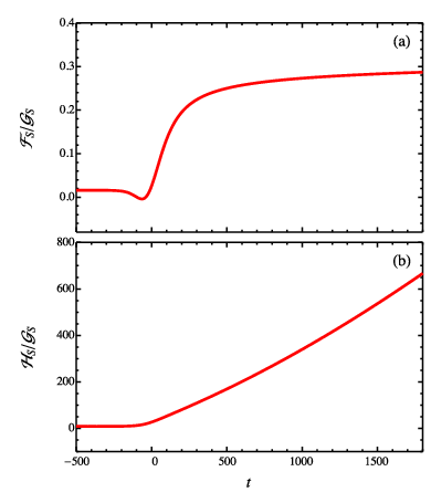
A numerical example of the Genesis-de Sitter transition is illustrated in Figs. 2 and 3. Our numerical calculation was performed as follows: we solve the evolution equations and with initial data satisfying , and confirm that the constraint is satisfied at each time step. In the numerical calculation, the parameters are given by , , , , and . The function is taken to be
| (82) |
with , , and . The background evolution is shown in Fig. 2. The evolution of the sound speed squared, , and the coefficient of in the dispersion relation is shown in Fig. 3. As pointed out in Ref. [26], flips the sign at the transition. The sound speed squared is positive except in this finite period. During the Genesis and subsequent de Sitter phases we have and , and therefore we may conclude that this model is stable.

Although we have thus obtained the stable example of the Genesis-de Sitter transition, the simple example (78) is not completely satisfactory if one would want successful gravitational reheating. Indeed, the condition (45) implies that , but for such . This problem can be evaded easily by the following small deformation of :
| (83) |
where is a parameter smaller than . The condition (45) now reads , i.e., , while
| (84) |
is positive for . The stability condition further restricts the allowed ranges of and . The necessary condition for stability is [see Eq. (77)]. This translates to , leading to = 4.8. Note that the small deformation of with does not change the background and perturbation dynamics of the Genesis and inflationary phases.
To illustrate the final stage of inflation, let us take
| (85) |
where the origin of time is shifted so that the end of inflation is given by . In the numerical plots presented in Figs. 4 and 5, the parameters are given by , , and , while the other parameters are taken to be the same as the previous example of the Genesis-de Sitter transition. It is found that . Again, we see that in the finite period around the transition. However, and remain positive all through the inflation and subsequent stages.
VI Discussion and conclusion
In this paper, we have introduced a generic description of Galilean Genesis in terms of the ADM Lagrangian and constructed a concrete realization of inflation preceded by Galilean Genesis, i.e., the scenario in which the universe starts from Minkowski spacetime in the asymptotic past and is connected smoothly to the inflationary phase followed by the graceful exit. Our model utilizes the recent extension of the Horndeski theory, which has the same number of propagating degrees of freedom as the Horndeski theory and thus can avoid Ostrogradski instabilities. This approach allows us to cover the background and perturbation evolution in all the three phases with the same single Lagrangian, as opposed to the effective field theory approach. In our scenario, the sound speed squared during the transition from the Genesis phase to inflation becomes negative for a short period. However, thanks to the nonlinear dispersion relation arising from the fourth-order derivative term in the quadratic action, modes with higher momenta are stable and the growth rate of perturbations with smaller momenta is finite and under control. It should also be noted that the sound speed of the primordial perturbations can be smaller than unity by choosing the parameter of the model appropriately.
Although we have constructed our inflation model in order to resolve the initial singularity and possible trans-Planckian problems by incorporating Galilean Genesis phase before inflation, we could make use of our model to realize the original Galilean Genesis scenario, which is an alternative to inflationary cosmology, simply by taking vanishingly short period of inflation there. As discussed in the Appendix, the sound speed squared becomes negative at the transition also in this case, but the instabilities are relevant only for small modes thanks to the term in the dispersion relation. Thus, the transition from the Genesis phase to the reheating stage is described in a healthy and controllable manner.
In fact, it would be fair to say that such a cosmology works quite well among the proposed alternatives to inflation, because, in contrast with the bouncing cosmology, in which all the would-be decaying modes in the expanding universe such as vector fluctuations and spatial anisotropy severely increase in an undesirable manner, the Genesis solution is an attractor and generation of nearly scale-invariant curvature perturbation is also possible with an appropriate choice of model parameters [18]. Since no first-order tensor perturbation is generated in this type of scenarios, detection of tensor perturbation with its amplitude larger than would be a smoking gun of inflation.
Acknowledgements.
This work was supported in part by the JSPS Grant-in-Aid for Scientific Research Nos. 24740161 (T.K.), 25287054 and 26610062 (M.Y.), 23340058 and 15H02082 (J.Y.).Appendix A Matching Genesis to the Reheating Phase

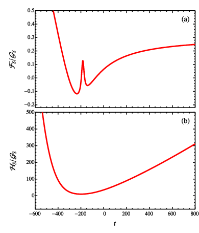
In the main text, we consider the scenario in which Galilean Genesis is followed by inflation. In this appendix, we will go back to the original motivation of Galilean Genesis and study how we can match smoothly the Genesis phase to the reheating phase. Our approach based on the ADM Lagrangian is quite useful in analyzing such a situation as well.
It is now obvious that by taking
| (86) |
and gluing the two functions smoothly at around , one can describe the Genesis-reheating transition. As a concrete example, we glue and smoothly at around and perform a numerical calculation as shown in Figs. 6 and 7. The other parameters are the same as those taken in the main text. As is expected, the numerical result here is much the same as the case where a duration of the intermediate inflationary phase is taken to be very short. In particular, becomes negative at the Genesis-reheating transition. The model is nevertheless stable since the conditions and remain satisfied.
References
- [1] A. A. Starobinsky, “A New Type of Isotropic Cosmological Models Without Singularity,” Phys. Lett. B 91, 99 (1980). K. Sato, “First Order Phase Transition of a Vacuum and Expansion of the Universe,” Mon. Not. Roy. Astron. Soc. 195, 467 (1981). A. H. Guth, “The Inflationary Universe: A Possible Solution to the Horizon and Flatness Problems,” Phys. Rev. D 23, 347 (1981). A. D. Linde, “A New Inflationary Universe Scenario: A Possible Solution of the Horizon, Flatness, Homogeneity, Isotropy and Primordial Monopole Problems,” Phys. Lett. B 108, 389 (1982).
- [2] For a review of inflation, see, e.g., J. Yokoyama, “Inflation: 1980-201X,” PTEP 2014, no. 6, 06B103 (2014).
- [3] V. F. Mukhanov and G. V. Chibisov, “Quantum Fluctuation and Nonsingular Universe. (In Russian),” JETP Lett. 33, 532 (1981) [Pisma Zh. Eksp. Teor. Fiz. 33, 549 (1981)]. A. A. Starobinsky, “Dynamics of Phase Transition in the New Inflationary Universe Scenario and Generation of Perturbations,” Phys. Lett. B 117, 175 (1982). S. W. Hawking, “The Development of Irregularities in a Single Bubble Inflationary Universe,” Phys. Lett. B 115, 295 (1982). A. H. Guth and S. Y. Pi, “Fluctuations in the New Inflationary Universe,” Phys. Rev. Lett. 49, 1110 (1982).
- [4] C. L. Bennett et al. [WMAP Collaboration], “Nine-Year Wilkinson Microwave Anisotropy Probe (WMAP) Observations: Final Maps and Results,” Astrophys. J. Suppl. 208, 20 (2013) [arXiv:1212.5225 [astro-ph.CO]].
- [5] G. Hinshaw et al. [WMAP Collaboration], “Nine-Year Wilkinson Microwave Anisotropy Probe (WMAP) Observations: Cosmological Parameter Results,” Astrophys. J. Suppl. 208, 19 (2013) [arXiv:1212.5226 [astro-ph.CO]].
- [6] P. A. R. Ade et al. [Planck Collaboration], “Planck 2013 results. I. Overview of products and scientific results,” Astron. Astrophys. 571, A1 (2014) [arXiv:1303.5062 [astro-ph.CO]].
- [7] P. A. R. Ade et al. [Planck Collaboration], “Planck 2013 results. XXII. Constraints on inflation,” Astron. Astrophys. 571, A22 (2014) [arXiv:1303.5082 [astro-ph.CO]].
- [8] H. V. Peiris et al. [WMAP Collaboration], Astrophys. J. Suppl. 148, 213 (2003) [astro-ph/0302225].
- [9] A. Borde and A. Vilenkin, “Singularities in inflationary cosmology: A Review,” Int. J. Mod. Phys. D 5, 813 (1996) [gr-qc/9612036].
- [10] V. A. Rubakov, “The Null Energy Condition and its violation,” Phys. Usp. 57, 128 (2014) [arXiv:1401.4024 [hep-th]].
- [11] I. Sawicki and A. Vikman, “Hidden Negative Energies in Strongly Accelerated universes,” Phys. Rev. D 87, no. 6, 067301 (2013) [arXiv:1209.2961 [astro-ph.CO]].
- [12] P. Creminelli, M. A. Luty, A. Nicolis and L. Senatore, “Starting the Universe: Stable Violation of the Null Energy Condition and Non-standard Cosmologies,” JHEP 0612, 080 (2006) [hep-th/0606090].
- [13] P. Creminelli, A. Nicolis and E. Trincherini, “Galilean Genesis: An Alternative to inflation,” JCAP 1011, 021 (2010) [arXiv:1007.0027 [hep-th]].
- [14] P. Creminelli, K. Hinterbichler, J. Khoury, A. Nicolis and E. Trincherini, “Subluminal Galilean Genesis,” JHEP 1302, 006 (2013) [arXiv:1209.3768 [hep-th]].
- [15] K. Hinterbichler, A. Joyce, J. Khoury and G. E. J. Miller, “DBI Realizations of the Pseudo-Conformal universe and Galilean Genesis Scenarios,” JCAP 1212, 030 (2012) [arXiv:1209.5742 [hep-th]].
- [16] K. Hinterbichler, A. Joyce, J. Khoury and G. E. J. Miller, “DBI Genesis: An Improved Violation of the Null Energy Condition,” Phys. Rev. Lett. 110, 241303 (2013) [arXiv:1212.3607 [hep-th]].
- [17] S. Nishi, T. Kobayashi, N. Tanahashi and M. Yamaguchi, “Cosmological matching conditions and galilean genesis in Horndeski’s theory,” JCAP 1403, 008 (2014) [arXiv:1401.1045 [hep-th]].
- [18] S. Nishi and T. Kobayashi, “Generalized Galilean Genesis,” JCAP 1503, no. 03, 057 (2015) [arXiv:1501.02553 [hep-th]].
- [19] L. Perreault Levasseur, R. Brandenberger and A. -C. Davis, “Defrosting in an Emergent Galileon Cosmology,” Phys. Rev. D 84, 103512 (2011) [arXiv:1105.5649 [astro-ph.CO]].
- [20] Y. Wang and R. Brandenberger, “Scale-Invariant Fluctuations from Galilean Genesis,” JCAP 1210, 021 (2012) [arXiv:1206.4309 [hep-th]].
- [21] D. A. Easson, I. Sawicki and A. Vikman, “When Matter Matters,” JCAP 1307, 014 (2013) [arXiv:1304.3903 [hep-th], arXiv:1304.3903].
- [22] V. A. Rubakov, “Consistent null-energy-condition violation: Towards creating a universe in the laboratory,” Phys. Rev. D 88, 044015 (2013) [arXiv:1305.2614 [hep-th]].
- [23] B. Elder, A. Joyce and J. Khoury, “From Satisfying to Violating the Null Energy Condition,” Phys. Rev. D 89, 044027 (2014) [arXiv:1311.5889 [hep-th]].
- [24] J. Martin and R. H. Brandenberger, “The TransPlanckian problem of inflationary cosmology,” Phys. Rev. D 63, 123501 (2001) [hep-th/0005209].
- [25] A. A. Starobinsky, “Robustness of the inflationary perturbation spectrum to transPlanckian physics,” Pisma Zh. Eksp. Teor. Fiz. 73, 415 (2001) [JETP Lett. 73, 371 (2001)] [astro-ph/0104043]; T. Tanaka, “A Comment on transPlanckian physics in inflationary universe,” astro-ph/0012431.
- [26] D. Pirtskhalava, L. Santoni, E. Trincherini and P. Uttayarat, “Inflation from Minkowski Space,” JHEP 1412, 151 (2014) [arXiv:1410.0882 [hep-th]].
- [27] G. W. Horndeski, “Second-order scalar-tensor field equations in a four-dimensional space,” Int. J. Theor. Phys. 10, 363 (1974).
- [28] C. Deffayet, X. Gao, D. A. Steer and G. Zahariade, “From k-essence to generalised Galileons,” Phys. Rev. D 84, 064039 (2011) [arXiv:1103.3260 [hep-th]].
- [29] T. Kobayashi, M. Yamaguchi and J. Yokoyama, “Generalized G-inflation: Inflation with the most general second-order field equations,” Prog. Theor. Phys. 126, 511 (2011) [arXiv:1105.5723 [hep-th]].
- [30] J. Gleyzes, D. Langlois, F. Piazza and F. Vernizzi, “Healthy theories beyond Horndeski,” arXiv:1404.6495 [hep-th].
- [31] M. Zumalacárregui and J. García-Bellido, “Transforming gravity: from derivative couplings to matter to second-order scalar-tensor theories beyond the Horndeski Lagrangian,” Phys. Rev. D 89, 064046 (2014) [arXiv:1308.4685 [gr-qc]].
- [32] X. Gao, “Unifying framework for scalar-tensor theories of gravity,” Phys. Rev. D 90, no. 8, 081501 (2014) [arXiv:1406.0822 [gr-qc]].
- [33] C. Lin, S. Mukohyama, R. Namba and R. Saitou, “Hamiltonian structure of scalar-tensor theories beyond Horndeski,” JCAP 1410, no. 10, 071 (2014) [arXiv:1408.0670 [hep-th]].
- [34] J. Gleyzes, D. Langlois, F. Piazza and F. Vernizzi, “Exploring gravitational theories beyond Horndeski,” JCAP 1502, no. 02, 018 (2015) [arXiv:1408.1952 [astro-ph.CO]].
- [35] X. Gao, “Hamiltonian analysis of spatially covariant gravity,” Phys. Rev. D 90, 104033 (2014) [arXiv:1409.6708 [gr-qc]].
- [36] M. Fasiello and S. Renaux-Petel, “Non-Gaussian inflationary shapes in theories beyond Horndeski,” JCAP 1410, no. 10, 037 (2014) [arXiv:1407.7280 [astro-ph.CO]].
- [37] L. Parker, “Particle creation in expanding universes,” Phys. Rev. Lett. 21, 562 (1968).
- [38] L. Parker, “Quantized fields and particle creation in expanding universes. 1.,” Phys. Rev. 183, 1057 (1969).
- [39] Y. B. Zeldovich and A. A. Starobinsky, “Particle production and vacuum polarization in an anisotropic gravitational field,” Sov. Phys. JETP 34, 1159 (1972) [Zh. Eksp. Teor. Fiz. 61, 2161 (1971)].
- [40] N. D. Birrell, P. C. W. Davies and L. H. Ford, “Effects of Field Interactions Upon Particle Creation in Robertson-walker universes,” J. Phys. A 13, 961 (1980).
- [41] L. H. Ford, “Gravitational Particle Creation and Inflation,” Phys. Rev. D 35, 2955 (1987).
- [42] T. Kunimitsu and J. Yokoyama, “Higgs condensation as an unwanted curvaton,” Phys. Rev. D 86, 083541 (2012) [arXiv:1208.2316 [hep-ph]].
- [43] K. Enqvist, S. Kasuya and A. Mazumdar, “MSSM Higgses as the source of reheating and all matter,” Phys. Rev. Lett. 93, 061301 (2004) [hep-ph/0311224].
- [44] J. Martin and R. H. Brandenberger, “The Corley-Jacobson dispersion relation and transPlanckian inflation,” Phys. Rev. D 65, 103514 (2002) [hep-th/0201189].
- [45] A. Ashoorioon, D. Chialva and U. Danielsson, “Effects of Nonlinear Dispersion Relations on Non-Gaussianities,” JCAP 1106, 034 (2011) [arXiv:1104.2338 [hep-th]].