Chiral low-energy physics from squashed branes in
deformed SYM
UWThPh-2015-7
Harold C. Steinacker11 1 harold.steinacker@univie.ac.at
Faculty of Physics, University of Vienna
Boltzmanngasse 5, A-1090 Vienna, Austria
Abstract
We discuss the low-energy physics which arises on stacks of squashed brane solutions of SYM, deformed by a cubic soft SUSY breaking potential. A brane configuration is found which leads to a low-energy physics similar to the standard model in the broken phase, assuming suitable VEV’s of the scalar zero modes. Due to the triple self-intersection of the branes, the matter content includes that of the MSSM with precisely 3 generations and right-handed neutrinos. No exotic quantum numbers arise, however there are extra chiral superfields with the quantum numbers of the Higgs doublets, the , and , whose fate depends on the details of the rich Higgs sector. The chiral low-energy sector is complemented by a heavy mirror sector with the opposite chiralities, as well as super-massive Kaluza-Klein towers completing the multiplets. The sectors are protected by two gauged global symmetries.
keywords: fuzzy extra dimensions; super-Yang-Mills; mirror fermions; chiral gauge theory
1 Introduction
Super-Yang-Mills (SYM) is the most (super)symmetric of all 4-dimensional field theories without gravity. As such it has played a prominent role ever since its discovery, even though it is usually considered as “too round” for real physics. More structure can be introduced by considering deformations of that model, notably by adding soft SUSY breaking terms to the potential. Then interesting patterns of spontaneous symmetry breaking can occur, inducing even more structure at low energy. A well-known example is the generation of fuzzy spheres, realized by the vacuum expectation values (VEV’s) of the matrix-valued scalar fields. Due to the Higgs effect, the model then behaves like a higher-dimensional model on [1, 2, 4, 3, 5, 7, 6, 8]. Recently, a much richer class of such solutions was found [9, 10] in the presence of a cubic SUSY-breaking potential corresponding to a holomorphic 3-form. These solutions can be interpreted as projected or “squashed” fuzzy coadjoint orbits of . Due to their self-intersecting geometry, they lead to 3 generations of massless fermions and scalar fields.
In this paper, we discuss these squashed brane solutions in more detail, and study some aspects of the resulting low-energy physics on stacks of such branes. Since there are massless scalar fields, it is natural (due to the presence of cubic interactions) to assume that some of them take non-trivial VEV’s. The main point to be emphasized here is that for suitable such VEV’s, the resulting low-energy sector behaves like a chiral gauge theory, in the sense that different chiralities of the fermionic (would-be) zero modes couple differently to the spontaneously broken massive gauge fields. Since this is a fundamental property of the standard model, that class of models becomes quite interesting for physics.
We first review and re-derive the fermionic and bosonic zero modes from a field-theory perspective, recovering results in [9]. The approach given here is based on two global symmetries which are respected by the background up to gauge transformations; these allow a coherent treatment of the bosonic and fermionic modes, and are very useful in understanding the interactions. The “regular” zero modes on a stack of branes can be organized in terms of a quiver, with 3 families of chiral superfields transforming in the bi-fundamental of gauge group arising on the coincident branes. They have specific weights in the weight lattice. Gauge fields and gauginos arise in vector supermultiplets. Nevertheless, the low-energy theory is not supersymmetric. These massless scalar modes will be dubbed “Higgs” modes henceforth.
Without attempting a full understanding of the rich Higgs sector in this paper, we consider some of the possible Higgs configurations, and elaborate the resulting physics in some detail using the new tools. In particular, we give a brane configuration which leads to the correct pattern of leptons and quarks coupling to the gauge fields of the standard model in its broken phase. This leads to an extension of the MSSM, where each chiral super-multiplet has an extra mirror copy with the opposite chirality, which acquires a higher (by assumption) mass from the mirror Higgs. The present scenario22 2 This is basically a refinement of an outline given in [10], in a slightly different more conservative setting. improves upon the analogous background solutions in [11] and related proposals [12] in several ways. First and foremost, there are necessarily 3 generations due to the triple self-interacting geometries, resulting in a family symmetry (which may subsequently be broken). Moreover, the chiral low-energy sector is protected from recombining with the massive mirror fermions due to two exact symmetries. These are combinations of the -symmetry and the gauge symmetry, which are preserved by the background. In this way, a stable chiral low-energy physics can arise from the underlying non-chiral theory. Furthermore, the scale of the mirror fermions can in principle be much higher than the electroweak scale, for large branes.
The present scenario is somewhat reminiscent of higher-dimensional string-theoretical (and field-theoretical) models such as [13, 14]. However it is much more radical and simple, since the chiral low-energy behavior is not put in by hand but arises from spontaneous symmetry breaking. Even if it may seem unlikely that such a scenario could be realistic, it is certainly worthwhile to explore the possible scope of these deformed models, given their special status in field theory.
Due to the complicated Higgs sector, no attempt is made in this paper to find the minima and to justify the assumed Higgs configuration. However, the basic result that certain Higgs configurations lead to chiral low-energy sector and a massive mirror sector is fully justified, and verified numerically. Also, the structure of leptons and quarks is very clear and convincing. However there is a rather complicated sector of modes with the quantum numbers of the two Higgs doublets and the electroweak gauge bosons, which is not worked out in detail. Some numerical computations are performed to gain some more insights, however this clearly requires more detailed investigations.
This paper is intended to be largely self-contained, and written from a field-theory perspective. Rather than just relying on the previous papers [9, 10], the necessary results are re-derived in a more transparent way, emphasizing the role of the two symmetries. Although this increases the length, the paper should be more accessible in this way.
2 Squashed branes in deformed SYM
We start with the action of SYM, which is organized most transparently in terms of 10-dimensional SYM reduced to 4 dimensions:
| (2.1) |
Here is the field strength, the covariant derivative, are 6 scalar fields, is a matrix-valued Majorana-Weyl (MW) spinor of dimensionally reduced to 4-dimensions, and arise from the 10-dimensional gamma matrices. All fields transform take values in and transform in the adjoint of the gauge symmetry. The global symmetry is manifest. It will be useful to work with dimensionless scalar fields labeled by the six roots33 3 Here we use field theory conventions, while in [9] group-theory friendly conventions are used. In particular, the are related to the standard basis of positive roots of used in group theory via , such that ; this is more natural here. of ,
| (2.2) |
with . These are viewed as points in forming a regular hexagon (see figure 3), with corresponding Weyl chambers defined by the Weyl group of reflections along these roots. Here has the dimension of a mass. Explicitly,
| (2.3) |
To introduce a scale and to allow non-trivial “brane” solutions, we add soft terms to the potential,
| (2.4) |
where
| (2.5) |
thereby fixing the scale . The cubic potential can be written as
| (2.6) |
corresponding to a holomorphic 3-form on . Rewritten in a real basis, this is recognized as the structure constants of projected to the root generators [9].
We will mostly set in this paper. Then SUSY is explicitly broken, and the global symmetry is broken to by the cubic term. However as show in appendix A, some supersymmetry can be preserved for a suitable choice of (and corresponding fermionic terms). More precisely, there is a specific deformation of SYM [15, 16, 3] with potential (2.5). However this requires to be outside of the domain which admits the squashed brane solutions of interest here. Nevertheless, this observation should help to understand the quantum corrections of the model, which is left for future work. Here we focus on the classical aspects of the model.
Perturbation of the background.
Let us add a perturbation to the background ,
| (2.7) |
This will lead to further symmetry breaking and interesting low-energy physics in the zero-mode sector of the background . The complete potential is easily worked out,
| (2.8) |
Here
| (2.9) |
can be viewed as gauge-fixing function in extra dimensions, and we define
| (2.10) | ||||
| (2.11) |
following [10], noting that
| (2.12) |
In particular, the equations of motion (eom) for the background can be written as
| (2.13) |
where is the 4-dimensional covariant d’Alembertian.
2.1 Squashed brane solutions
It is well-known that the above potential has fuzzy sphere solutions where are generators of [1, 17, 2, 3, 4, 5, 6, 7]. However as shown in [9], there are also solutions with much richer structure corresponding to (stacks of) squashed fuzzy coadjoint orbits , obtained by the following ansatz
| (2.14) |
Here
| (2.15) |
are root generators of , is any representation on , and are the simple roots with . In these conventions, the Lie algebra relations are
| (2.16) |
with and where denotes the Killing form of . Using these Lie algebra relations, the equations of motion (2.13) become
| (2.17) |
Assuming for simplicity, these equations have the non-trivial solution
| (2.18) |
For an irreducible representation (irrep) with highest weight acting on , these solutions can be interpreted as quantized or fuzzy coadjoint orbits projected to along two Cartan generators [9]. Generically these are 6-dimensional (fuzzy) varieties, while for and they are 4-dimensional projections of (fuzzy) . Here denotes the Dynkin labels of . Such a “squashed” has a triple self-intersection at the origin, as visualized in figure 1.
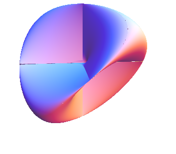
We will see that pairs of fermionic zero modes arise at the intersections, connecting the different sheets.
To organize the degrees of freedom, we note that these solutions defines an embedding , which acts via the adjoint on all the fields in the theory. Decomposing the -valued fields into harmonics i.e. irreps of this
| (2.19) |
(here denotes the highest weight irreps) allows to understand the physics of the fluctuations on such a background, even though the gauge symmetry is broken completely for irreducible . In particular, the gauge transformations act on the scalar fields as
| (2.20) |
(here is the -dimensional representation of ). Now restrict to the Cartan subalgebra or the torus , which is sufficient to specify the weights in the various harmonics. Then the last term in (2.20) vanishes, and the six scalar fields transform linearly, corresponding to the six non-zero weights in of . This organization will be very useful.
The potential has a global symmetry, which is broken to or in the presence of masses . We denote with the traceless generator which has eigenvalue on and on the with , or more formally
| (2.21) |
Then , and the action of on the scalar fields coincides with the adjoint action of the Cartan generators of . In other words, the background is annihilated by the following generators
| (2.22) |
which satisfy , and generate a symmetry of the background. Their charges are obtained by adding the (rescaled and rotated, cf. figure 4) weights of to the non-zero weights of of . In particular, the charges of are points in the weight lattice of . This will be very important to characterize and protect the zero modes.
Now we can understand the Goldstone bosons arising from the broken global symmetries. The background breaks the global symmetry, but the traceless with generators are equivalent to gauge transformations (i.e. “gauged“). Therefore there will be only physical Goldstone bosons, as the two modes are eaten by the massive gauge bosons. These 6 physical Goldstone bosons are identified in appendix B with the 6 exceptional zero modes in the as discussed below.
Finally, the background admits a symmetry, which cyclically permutes the . This is part of the symmetry, and also part of the Weyl group44 4 The potential is in fact invariant under the full Weyl group of . of . It is also interesting to recall that the global is anomalous, and there is an associated Wess-Zumino term [18]. This might be important for the effective description of the 6 physical Goldstone bosons.
2.2 Scalar zero modes on squashed branes
Let from now on. Then the squashed brane backgrounds admit a number of zero modes . To see this, we note that the bilinear form defined by on a background (2.14) can be simplified e.g. as follows
| (2.23) |
using and . This has precisely the form of the quadratic contribution from the cubic potential (2.8). Therefore the quadratic terms in the potential can be written as
| (2.24) |
It was shown in [9] that is positive semi-definite for all representations . The zero modes of fall into two classes, denoted as regular and exceptional zero modes. Let us first focus on the regular zero modes, which are given by solutions of the decoupling condition [9, 10]
| (2.25) |
Here we shall provide a group-theoretic characterization of the regular zero modes, which implies (2.25); it is then straightforward to show that they are zero modes. Recall that the background respects the generators55 5 This symmetry was also used in [10] to classify excitations on spinning brane backgrounds. (2.22), and consider the ”-parity“ generator in defined by
| (2.26) |
which is broken by the cubic potential. Then
| (2.27) |
Now fix some highest weight module , and consider the set of weights of , given by the 6 nonzero weights of minus the weights in . Among these, consider the 6 extremal weights66 6 These are the corners of the convex set of weights in , or equivalently of the maximal irrep in . The conventions differ in an inessential way from the ones in [10]. , and denote the corresponding modes as
| (2.28) |
Here is an extremal weight vector with weight in . These have charge under the , corresponding to a point of the weight lattice in (the interior of) the Weyl chamber of . These are the regular zero modes. They have eigenvalue determined by the parity of the Weyl chamber of . Since there is only one such state for any such (extremal!) and preserves , (2.27) implies that
| (2.29) |
Using the extremal weight property, it is then easy to verify that these are zero modes
| (2.30) |
e.g. for , we have (cf.[10])
| (2.31) |
hence (2.30) follows from . We will find superpartners of these regular zero modes in section 4. Particular examples of such modes are given by
| (2.32) |
Observe that they have eigenvalue determined by the Weyl chamber of . A possible background with such a “Higgs” switched on would then be
| (2.33) |
On a single squashed brane, these exhausts all regular zero modes. Observe that there are 6 such zero modes even for degenerate such as . Some intuition can be gained by noting that the regular zero modes with maximal on squashed link the 3 intersecting sheets at the origin, with polarization along the common [9]. More generally, the regular zero modes can be interpreted as strings linking these sheets, shifted along their intersection77 7 For examples of such string-like modes see e.g. [19]..
For harmonics with and , there are in addition 3 exceptional zero modes [9] with resp. , which have mixed polarizations. The most important among these arise for : these correspond to the 6 physical Goldstone bosons which arise from as discussed above, see appendix B. The full set of zero modes for squashed branes can then be obtained from the mode decomposition
| (2.34) |
assuming . There is a set of 6 exceptional zero modes in given by the Goldstone bosons, and typically 3 exceptional zero modes for , or for .
From now on, we will collectively denote the set of these scalar (“would-be”) zero modes as Higgs sector, anticipating that they may acquire some VEV or some mass.
Higgs connecting different branes.
Now consider backgrounds consisting of several branes, described by reducible representations in (2.14). For example, the matrix modes on a stack consisting of one and one brane decompose as
| (2.35) |
To be specific, assume that and . Then , each leading to 6 regular zero modes with from , 6 regular zero modes with from corresponding to translations in the internal , and 6 exceptional zero modes with from corresponding to the Goldstone bosons. Here denotes the set of weights given by the action of the Weyl group on . On the other hand, the regular modes connecting different branes can be written as
| (2.36) |
where are weights in , and is in the Weyl chamber opposite to . This leads to 6 regular zero modes with from , 6 regular zero modes with from , and 3 exceptional zero modes with from . Since the can be viewed as coherent states on located at the origin [9], the modes are strings linking the sheets of and with a 2-dimensional intersection at the origin, while the modes are strings linking coinciding sheets at the origin. Finally, the modes connecting with a point brane arise from
| (2.37) |
leading to 6 regular zero modes with , and 3 exceptional zero modes with .
3 A standard-model-like brane configuration
Now consider a background consisting of two coincident (isomorphic) branes , and two additional (typically different) branes and . We assume that the scale of these branes is very high. Furthermore we add a “leptonic” point brane , and 3 “baryonic” point branes . Hence the matrices of SYM act on
| (3.1) |
If realized within SYM (instead of ), this background admits a gauge symmetry, or if . Such stacks of branes might be bound by quantum effects in SYM, which are related to supergravity and typically induce an attractive interaction between branes with different flux [20, 21, 22, 23].
Now we switch on some “Higgs” links between these branes, realized by (would-be) zero modes linking some extremal states of the various as in (2.36),
| (3.2) |
First, assume that the point-brane is linked to the extremal weight states of as in (2.37),
| (3.3) |
dropping the polarization indices. Assuming that the scale of is high88 8 We might as well consider as a single brane., the unbroken gauge symmetry is reduced to , where is generated by . To write this in a more suggestive form, we introduce the hypercharge generator
| (3.4) |
and
| (3.5) |
(as in [11]), where
| (3.6) |
will act as chirality in the light sector due to (4.31). Then the unbroken gauge symmetry can be written as , where and will be anomalous in the light sector but not in the full model, and is the trace-. The latter can be dropped in SYM, but acquires an interesting role related to gravity in the IKKT matrix model [24]. This leaves exactly the gauge group of the standard model , extended by , and possibly . The will also be broken by the electroweak Higgs as elaborated below. All other gauge bosons are massive with mass set by the scale or ; we will ignore these from now on.
Now assume that some “electroweak” Higgs arise such that the 4 squashed branes form two bound states
| (3.7) |
as sketched in figure 2.

For example, we could have and . Dropping indices, we can write the corresponding Higgs suggestively as
| (3.8) |
connecting some of their extremal weight states of and Thus and can be viewed as non-vanishing entries of two doublets as in the MSSM (5.5), with
| (3.9) |
We assume that the scale of the branes is much larger than the (electroweak) scale of the Higgs, and , so that we can neglect the back-reaction of the Higgs on the branes. This defines the background under consideration. The 3 coincident “baryonic” point branes remain disconnected from the rest. As discussed above, such squashed branes are solutions of our model. The above Higgs are part of the zero mode sector, and we simply assume that they acquire some VEV.
Once these Higgs fields and are switched on, the gauge symmetry is broken99 9 Note that nonabelian VEVs in the scalar sector do reduce the rank of the gauge group. to , where is the baryon number, and
| (3.10) |
is the electric charge generator. Here indicate the which is part of and , respectively. Note that is traceless provided . We will see that and give the correct charge assignment of the standard model; in particular, we note the Gell-Mann-Nishjima formula
| (3.11) |
Thus the low-energy broken gauge modes are given by three massive generators of identified as and , and the mode generated by . To elaborate the masses of these low-energy gauge bosons, we decompose the Hilbert space of scalar fields on the two as
| (3.12) |
where are the functions on . Then the bosons arise from the -valued gauge fields which are proportional to on . The components of the gauge fields are accordingly given by
| (3.13) |
where
| (3.14) |
They couple to the fermionic zero modes
| (3.15) |
and similarly to the Higgs fields
| (3.16) |
As explained in detail below, these reproduce precisely the couplings and charges of the standard model. We can therefore identify the gauge fields , etc. with those of the the standard model, where is the coupling constant, and is the coupling constant. The coupling constants of the gauge bosons are therefore given by
| (3.17) |
The appropriate normalization is obtained such that the Lagrangian of the gauge fields is
| (3.18) |
i.e. , which gives
| (3.19) |
Then the masses of the gauge bosons are obtained from
| (3.20) |
where the covariant derivatives of scalar fields (3.8) are explicitly
| (3.21) |
The boson is identified as the combination of and which acquires a mass,
| (3.22) |
On the other hand, (3.10) guarantees that remains exactly massless, since and are disconnected. The masses are obtained from
| (3.23) |
for . Here is evaluated using the explicit form (3.21) of connecting the extremal weight states of the squashed branes, and does not contribute any -dependent factors1010 10 This is an essential improvement compared with the background in [11], which lead to a factor at this point, and to an equal scale of the mirror fermions and bosons.. We can then read off the tree-level and bosons masses,
| (3.24) |
All scales are set by . Note that as long as , is much lower than any of the higher KK gauge bosons which start at , where is the lowest eigenvalue of on . The photon and the -boson are now identified as usual
This gives the Weinberg angle
| (3.25) |
E.g. for this gives , for this gives , and for this gives . These are of course tree-level formulae which should be viewed as GUT values at very high energies.
These formulae have to be generalized in the presence of several Higgs components, in particular and which couple to the mirror fermions and standard-model fermions, respectively. All of them contribute to the mass as above, and must be taken into account accordingly.
To put this into perspective, consider briefly the coupling of the Higgs to the fermionic zero modes (which are discussed in detail below). We will see that the off-diagonal fermionic zero modes connecting with or have the structure
| (3.26) |
and the Yukawa couplings among these arise from
| (3.27) |
The trace gives no extra factor since the fermions are made from coherent states, similar as the bosonic modes in (3.23). Therefore the fermion mass is given by
| (3.28) |
which is much larger than the scale (3.24) for large branes with . This implies that the mirror fermions can be much heavier than the scale, which is essential, and resolves one of the main issues in [11]. On the other hand, this also entails that the coupling is considerably larger than the electroweak coupling . In the present paper, we focus on minimal or small branes.
In the next section we discuss the fermionic zero modes on such a background, and show how the fermions of the standard model can arise.
4 Fermionic zero modes
Now we turn to the fermionic zero modes, which provide the matter content of the low-energy field theory on the squashed backgrounds. The basic results are obtained in [9, 10], however we emphasize again their group-theoretical organization which makes the relation with the scalar zero modes manifest.
The internal Dirac operator on a background describes a stack of branes has the form
| (4.1) |
where the spinorial ladder operators
| (4.2) |
and satisfy
| (4.3) |
We recall the traceless generators of the , and introduce their spinorial representation
| (4.4) |
with . The 8 states in a Dirac spinor of transform in the of , and decompose into under . The 6 non-vanishing charges of thus form a regular hexagon (just like the scalar fields )
| (4.5) |
while two singlet “gaugino” states
| (4.6) |
have vanishing charge . The spinors with have definite chirality determined by
| (4.7) |
where is the trace- generator acting on the spinors corresponding to (2.26).
Now we can exploit the fact that the background preserves the symmetries (2.22). This implies that the Dirac operator commutes with
| (4.8) |
in analogy to (2.22). As in section 2.2, it follows that for each irreducible , has 6 zero modes labeled by
| (4.9) |
which are in one-to-one correspondence to the extremal weights of the . Here is some extremal weight vector in . This follows from 1) the multiplicity of the extremal weight states is one, 2) they are eigenvectors of , and 3)
| (4.10) |
In particular, these can be viewed as superpartners the bosonic regular zero modes (2.30), with the same charge under . For example,
| (4.11) |
where is the highest weight vector of . This can easily be verified directly using the form (4.1) of the Dirac operator, together with
| (4.12) |
These states are visualized1111 11 This picture differs from figure 1 in [10] due to a different choice of roots. in figure 3. They fall into chirality classes and with well-defined internal chirality
| (4.13) |
determined by the parity of the Weyl chamber of ; recall that the reflections along the divide weight space into the 6 Weyl chambers of . Now is in the same Weyl chamber as , and in the opposite Weyl chamber as the gauge charge of the matrix wave-function . Thus the chirality of is determined by the parity of , hence1212 12 This is strictly true only for which are not on the border of two Weyl chambers. Otherwise, there are two zero modes with opposite chirality associated to . by . This is an important statement, because it signals a chiral behavior of the low-energy gauge theory. All this is consistent with the vanishing index of .

It turns out that there are no other fermionic zero modes besides these extremal zero modes, except for the trivial gaugino modes with . The remaining fermionic modes (including the gaugino modes for ) acquire “Kaluza-Klein” masses with scale set by . In particular, there are no fermionic zero modes corresponding to the exceptional scalar zero modes, hence supersymmetry is manifestly broken even in the low-energy spectrum.
So far, we only discussed the internal spinor structure of the zero modes. Taking into account the 10D Majorana-Weyl condition , this translates directly to the space-time spinor structure. It is easy to see (cf. [9]) that the extremal modes and are related by the internal charge conjugation and have opposite chirality,
| (4.14) |
Let us use the short notation , where are the roots of . Taking into account the Majorana-Weyl condition, the corresponding solutions of the full Dirac operator have the form
| (4.15) |
where the four-dimensional spinors satisfy
| (4.16) |
and have specific chirality
| (4.17) |
This means that the are not independent, as determines . We can expand the general solution in terms of plane wave Weyl spinors on with momentum ,
| (4.18) |
This can be viewed in terms of three 4-dimensional Weyl spinors , which naturally form 3 chiral supermultiplets with the corresponding bosonic zero modes.
Together with the relation between the internal chirality and the charges established above, it follows that the fermionic zero modes cannot acquire any mass terms even at the quantum level, as long as the is unbroken. There are simply no other modes available with the opposite and the same 4D chirality to form a mass term in 4 dimensions. This holds even in the presence of mass terms such as in (2.5) or their fermionic analogs.
Since the above analysis is based entirely on group theory, the classification of zero modes carries over immediately to stacks of branes. The results can then be summarized by stating that a quiver gauge theory arises on stack of squashed branes , with gauge group on each node and arrows corresponding to chiral superfields labeled by the extremal weights obtained by adding the six non-vanishing weights to the (negative) weights of . Fields with opposite weights are conjugates of each other. The trivial modes on each node lead to supermultiplets. However, this quiver does not give the full story, as there are exceptional scalar zero modes, heavy fields, and non-supersymmetric interactions which arise from the parent theory.
We will restrict ourselves to the fermionic zero modes from now on. We emphasize again that all fermionic zero modes come in 3 generations, except for the two gaugino modes which arise for .
4.1 Higgs fields and Yukawa couplings on minimal branes
Adding a Higgs to the background , the fermionic zero modes may acquire masses through Yukawa couplings arising from ,
| (4.19) |
These Yukawas are non-vanishing only if the charges of the three fields under add up to zero, which provides a strong constraint for these couplings. Since the gaugino modes (4.6) arise only for the trivial modes, they cannot contribute any non-vanishing Yukawas in the zero mode sector. Together with the symmetry, this implies that the non-vanishing Yukawas in the zero-mode sector have the following form
| (4.20) |
or its conjugate. In particular, the -parity of are equal. However, we do not know which Higgs assume a non-vanishing VEV. This should be determined largely by the cubic flux term (2.6), while the quartic potential will stabilization the Higgs, as discussed in section 5.2. Note that the structure of the Yukawa coupling (4.20) is very similar to the cubic flux term, which also couples only modes with the same -parity. Since the flux term is odd, it is plausible that non-trivial solutions with non-vanishing Yukawa couplings arise, with separate sectors. The latter will correspond to the light sector and the mirror sector below. However, a detailed analysis is beyond the scope of the present paper. We will thus make some simplifying assumptions in the following, in an attempt to identify physically interesting configurations for such Higgs and Yukawa couplings.
Our first assumption is that there are no Higgs modes on any given (linking a brane with itself). We restrict ourselves to Higgs fields arising as links between branes and in (3.7). This suffices to exhibit the separation into light and mirror fermions.
Minimal branes and Higgs.
We restrict ourselves to the minimal squashed branes in this paper, with and . Then among all possible Higgs modes linking and in (2.36), we focus on the regular zero modes with
| (4.21) |
with antisymmetric1313 13 the symmetric combination is part of . , and the modes
| (4.22) |
which are determined by conjugation. They link adjacent weights and of and , interpreted as strings linking the sheets of and [9]. We will ignore the remaining regular zero modes with and the 3 exceptional zero modes with and here, since they would not lead to Yukawas between the fermionic zero modes relevant to the SM. However they may give a mass to some of the extra (unwanted) fermions which arise besides the standard-model fermions, and should be taken into account eventually in a more complete analysis.
Consider these Higgs modes (4.21) in more detail. Since is the conjugate representation to , the latter are determined by the 3+3 independent modes by conjugation. Equivalently, we can consider the three modes with and the three modes with as independent modes, which determine the remaining modes by conjugation. Explicitly, writing the background1414 14 The minus in the second term reflects the fact that the generators of conjugate representations are related by minus transposition. as
| (4.23) |
(cyclically) where and etc., these six independent Higgs fields are
| (4.24) |
for , which determine their conjugates , (see figure 4 and 5). The superscripts indicate the -parity .

Hence they are parametrized by 3 + 3 (complex) fields and , which will be referred to as “Higgs” and “mirror Higgs”.
Now we assume that only , or more generally . In other words, the -parity of the Higgs with is positive, and the -parity of the Higgs with is negative. This is the crucial assumption, which will lead to a chiral low-energy theory. It is reasonable, because the flux term only couples fields with the same -parity; however a detailed investigation is left for future work. We will see that under this assumption, the “mirror Higgs” gives a large mass to the “mirror” sector of the standard model, leaving the chiral standard model with massless chiral fermions (and some extra fields) at low energies. The (small) modes then play the role of the low-energy Higgs, giving mass to these standard-model fermions as usual.
Finally, consider the Higgs (3.3) connecting a minimal brane with a “point” brane . Similar as the Higgs connecting minimal branes, we can organize them in terms of 3+3 modes with -parity
| (4.25) |
in the basis (4.24), and their conjugates. Those may be switched on independent of each other. There are also 3 exceptional scalar zero modes with , which we will ignore here.
Fermions between branes and points.
Now consider the fermionic zero modes in more detail. The zero modes linking and with a point brane are given by
| (4.26) |
These are 6 zero modes with and 6 zero modes with , with chirality determined by the -parity of . The Yukawa coupling of two such fermionic zero modes with the Higgs fields is non-vanishing only if the charges of and add up to that of . A direct inspection of the weight lattice (see figure 5)

shows that has indeed solutions provided the parities of and are equal and opposite to that of . There are no other couplings among these modes, consistent with the general discussion following (4.20). Together with the above assumption on the Higgs, this means that Yukawa couplings arise only between left-handed with and right-handed with , mediated by with . Hence the fermions (4.26) separate into “mirror” fermions
| (4.27) |
which acquire a large mass of order , while the remaining modes remain massless and constitute the “light” sector
| (4.28) |
To summarize, the light fermions are left-handed links from to , and right-handed links from to . If , then these light fermions couple among themselves and acquire a mass of order .
Now the crucial point is that the zero modes (4.26) with and are distinguished by their gauge charges:
| (4.29) |
where is the gauge generator (spontaneously broken by ) which assigns the charges to the branes and . Combining these results, we conclude that
| (4.30) |
hence
| (4.31) |
using (4.17). This means that the low-energy fermions are chiral as seen by the spontaneously broken gauge fields, just like the fermions in the standard model (in the broken phase). The basic result (4.30) will be verified numerically in section 6, and the relation with the standard model will be made more specific below.
Finally assume that in addition (4.25) is switched on, connecting with . This will induce Yukawa couplings of with fermions on and on , and possibly Yukawa couplings of with . Switching on or selectively, this should give a mass to while leaving the light fermions massless. This is desirable since it will give mass to , however a detailed investigation is left for future work.
Fermions on and between branes.
Now consider the fermionic zero modes linking different branes. They are in one-to-one correspondence with the regular scalar zero modes discussed above. In particular, the zero modes connecting two minimal branes with have the form
| (4.32) |
corresponding to (2.36), where stands for the spinor (4.5) with weight . This leads to 6 zero modes with and 6 zero modes with . The latter are the superpartners of the Higgs fields (4.22).
There are also fermionic zero modes on some minimal branes ,
| (4.33) |
Six of these have , and 8 are trivial modes with . If and are connected with a Higgs as above, then Yukawa couplings with structure and arise, giving mass to some of these fermions. Rather than attempting a detailed analytical explanation here, we will analyze this numerically in the next section.
5 Standard model fermions from branes
Now we apply these results to the brane configuration for the standard model (3.7). Consider the off-diagonal fermions linking the branes. In the basis , we denote these fermions as
| (5.1) |
The fermions of the SM arise as links between the point branes and and resp. , i.e.
| (5.2) |
as well as the right-handed leptons and quarks. Furthermore there are slots for the Higgsinos as in the MSSM. The charge generators
| (5.3) |
assign the following quantum numbers to these off-diagonal modes
| (5.4) |
(the assignment is obvious, hence dropped). All quantum numbers of the standard model are correctly reproduced (cf. [34, 20]), and 3 families arise automatically due to the symmetry. The Yukawa couplings may of course break the , and will be discussed below. Thus the leptons arise as fermions linking or with , and the quarks arise as fermions linking or with .
All these modes have scalar superpartners given by the regular scalar zero modes. In particular, the two Higgs doublets1515 15 Unfortunately there is a conflict with the standard particle physics conventions, where the role of the is reversed, as is seen from their quantum numbers (5.4). The present notation is forced upon us by (3.7).
| (5.5) |
with (as in the standard model) and (as in the MSSM) fit into the above matrix structure as
| (5.6) |
This indeed leads to the desired pattern of electroweak symmetry breaking, as shown in section 3. We also exhibit the “sterile” Higgs , which is a singlet under the standard model gauge group, occupying the same slot as . The chiralities and masses of the fermions depend on the Higgs expectation values. We will see in the next section that for , the low-energy fermions linking point branes with are left-handed, and those linking with are right-handed. The fermions with the opposite chiralities – which necessarily exist due to the vanishing index in SYM – acquire a large mass terms of order , and are therefore invisible at low energies. Thus the fermions of the standard model have indeed the appropriate chirality at low energies, as suggested by their names etc. Finally, recall that the modes in the lower-diagonal part of the matrices are identified by the MW condition with the upper-diagonal ones, and therefore do not constitute independent degrees of freedom.
It is remarkable that no exotic charges arise: all the charges in (5.4) correspond to the charges of the standard model, extended by the second Higgs doublet and the sterile . Thus we recover all fermions in the MSSM (including e.g. gluinos, winos and binos), extended by
| (5.7) |
which has the same quantum numbers as the quarks (but it comes with both chiralities), and
| (5.8) |
which has the same quantum numbers as . This degeneracy can be understood by viewing as a single brane linked via . Thus may mix with , and with , and similarly may mix with neutral Higgsino at low energies. The can be viewed as superpartner of the would-be gauge bosons connecting and if . Finally there are a number of fermions which are neutral under the SM gauge groups. This includes the superpartner of the (broken) gauge field
| (5.9) |
some diagonal “neutralino” modes on and , and of course . The multiplets come in several incarnations corresponding to different modes, which may acquire a mass from the Higgs(es). This is discussed next.
One might absorb the extra fields and by replacing by a single brane , as discussed in section 3. However, then there are typically extra modes connecting the extended branes. The main reason for keeping separate is to keep things transparent by working with minimal branes and point branes .
5.1 Chiral fermions and Yukawas on the standard model branes
Now we apply our results on the Yukawa couplings to this brane configuration, with and . In particular, we assume that are linked by Higgs as above, and similarly for .
Consider first the fermions linking the point branes with or . Assuming that , the results of the previous section imply that these separate into light fermions with masses of order , and heavy mirror fermions with masses of order . This leaves only the light fermions at low energy, which comprise left-handed fermions linking to , and right-handed fermions linking to . They correspond to the standard-model-like chiral leptons and quarks. The mirror fermions have the same S.M. quantum numbers but the opposite chiralities, distinguished by the quantum nmbers. Due to the simple mode decomposition1616 16 This holds also for genral non-minimal branes, as long as are point branes. (4.26), we get precisely the same quark and lepton with their superpartners as in the MSSM, plus their mirror modes at higher energies (which also form supermultiplets).
Now consider the low-energy fermions which arise on the and branes (i.e. in the upper-left block in (5.1)). This includes the superpartners of the electroweak sector, such as Higgsinos, Winos, Binos, charginos and neutralinos, as well as the . They come in different multiplets corresponding to the different modes in (4.32). Their precise Yukawa couplings and masses in this sector are rather complicated and will not be discussed in detail here; some illustrative numerical results are given in the next section. Since the modes come as multiplets, there are also 3 generations of chiral supermultiplets corresponding to the and bosons. The numerical results indicate that some but not all of these acquire a mass from the mirror Higgs , which suggests that some of the other Higgs discussed in section 4.1 should also acquire a VEV. We leave this for further investigations.
Finally some fermionic would-be zero modes arise within the 4 point branes . This includes gluinos with , the color triplet (5.7) which is similar to , and the singlets on (5.9). We only discuss some aspects here, postponing a detailed analysis to future work. First, the Higgs with should lead to a Yukawa coupling of the with the modes with , and give a large mass to both and (except for the two gaugino polarizations (4.6) of ). Similarly, the might couple to via , (except for the two gaugino polarizations of ), giving a mass to and . It is tempting to speculate that the large Yukawa couplings of the top quark may be related to the presence of . The fate of the two gaugino polarizations of and is unclear. In any case, the sector containing and is rather complex and should be studied elsewhere.
Due to the different parity modes of and , it is possible that e.g. acquires a large mass but not its mirror . Then the seesaw mechanism would apply to the physical neutrinos but not to the mirror neutrinos, and no new massless neutrinos would be introduced.
The main result here is the separation of leptons and quarks into light chiral and heavy mirror sectors, assuming a suitable Higgs configuration. The crucial decoupling of the light and mirror sector is guaranteed by the global symmetry, and persists in the presence of explicit mass terms respecting that symmetry, such as in the model discussed in appendix A. This mechanism will be verified numerically below, along with some illustrative sample computations for the remaining sectors.
Extra ’s and anomalies.
In the presence of chiral fermions, the gauge fields arising on backgrounds consisting of several branes deserve special attention. Consider first the field theory setting at hand. Assuming that the mirror Higgs is much larger than the light Higgs as above, some of these ’s aquire anomalous contributions from the low-energy sector (i.e. after integrating out the massive mirror fermions). In the present brane configuration this is the case for the and the fields. However, this anomaly from the light sector is canceled precisely by the anomaly from the mirror sector, so that there is no overall anomaly, in accordance with t’Hooft anomaly matching and the fact that SYM has no gauge anomalies. In particular, the gauge field remains massless in this model.
To get a better perspective on these ’s, it is useful to recall the analogous situation in string theory. The present softly broken SYM model would arise “locally” e.g. on stacks of -branes in a suitable flux background, cf. [25, 26, 13]. Then some of these ’s are anomalous at low energy and acquire a mass through a Stückelberg mechanism [29, 30, 31, 27, 32, 28], absorbing the corresponding Stückelberg field or axion which arises from the RR fields in string theory. This is a manifestation of the Green-Schwarz anomaly cancellation. In the present field theory setting, there is no manifest axion, hence the correspondence with the string theory case is not fully realized. However for analogous backgrounds in noncommutative in the IKKT matrix model, axion-like fields do arise [33], as expected from the relation with string theory. One may then hope that an analogous Stückelberg mechanism applies and renders some of these ’s massive, however the details remain to be understood.
5.2 Aspects of the Higgs potential
Now consider the interacting potential for the Higgs i.e. the scalar zero modes on a background solution . The linear term in vanishes, so that the effective potential for obtained from (2.8) is
| (5.10) |
The cubic interaction arising from the quartic term can be written in different ways
| (5.11) |
using the Jacobi identity, , and the gauge condition . The latter is a special case of the following identities
| (5.12) |
and
| (5.13) |
for the regular zero modes. These follow easily from their extremal weight property, see [10]. Since one of these two conditions is always satisfied for any pair of roots of , this cubic term vanishes for the regular zero-modes, so that their interaction potential is
| (5.14) |
where the quadratic term vanishes in the absence of mass terms. The argument applies also to Higgs modes connecting stacks of branes, as long as the are proportional to generators. Note that the Higgs potential has similar structure as our starting point (2.5). Although a full analysis of this potential is beyond the scope of this paper, it is plausible that the cubic flux term again induces a non-trivial VEV to some of the Higgs modes, which are stabilized by the quartic term. A deformation of the branes by quantum corrections or mass terms1717 17 Another conceivable mechanism is a rotation of the branes, see [10]. might also play an important role here.
The above argument for (5.11) to vanish does not apply to the exceptional zero modes. Among those, the Goldstone bosons are exactly flat directions, but the (or conjugate) modes connecting with might lead to non-trivial cubic terms. Again, this needs to be studied in more detail elsewhere.
Finally, we emphasize that even though the Higgs sector consists of many distinct fields etc., there should nevertheless be one lowest Higgs fluctuation mode around the common minimum, which is likely a combination of all the and modes. Thus the assumption is not in obvious conflict with observation. At higher energies of course, several distinct Higgs modes will necessarily show up.
6 Numerical results and checks
Since the detailed structure of the various zero modes and their Yukawa couplings is quite complicated, a background consisting of two minimal branes with Higgs and an extra point brane was implemented in Mathematica. We consider two branes linked by a Higgs and as in (4.24), and add a point brane to this configuration. We are interested in the Yukawa couplings and the masses of the fermions in this background, which is determined by the low-energy spectrum and the eigenmodes of the Dirac operator acting on spinors
| (6.1) |
Here we note that and
| (6.2) |
Due to the MW condition, these two contributions are identified, so that the last term in (6.1) reduces to ; a similar reduction should be applied to all modes. The lowest eigenvalues and multiplets of the Dirac operator on the background were obtained as a function of the parameters , for . Their eigenvalues have also been determined. The detailed results are as follows:
6.1 Fermions linking to a point brane
The most interesting sector are the fermionic links (6.2) of a point brane to , which we discuss first. They are determined by the Dirac operator acting on spinors
| (6.3) |
as in (4.26). In the absence of any Higgs , there are 6+6 exact zero modes as expected on , and the non-zero eigenvalues of are of order . Switching on but leaving , six of the would-be zero modes (‘‘mirror fermions’’) acquire non-vanishing eigenvalues1818 18 these specific eigenvalues are not hard to understand. , while exact zero modes remain. The latter are the “light fermions” which constitute the fermions in the standard model, and one can verify that (4.30) holds1919 19 This holds to an excellent approximation as long as the background is undeformed, i.e. ., i.e. their chirality is measured by . These are indeed modes with . Switching on also , these light fermions acquire eigenvalues approximately given by . This precisely confirms the analysis in the previous sections, which means that the low-energy leptons and quarks on the SM brane configurations have indeed the appropriate chiral structure.
6.2 Fermions within
Now consider the fermions on , which live in
| (6.4) |
In the absence of any Higgs , we find indeed exact zero modes, which are the superpartners of the regular scalar zero modes in this sector. The preserve the branes, while the modes connect the two branes. The remaining non-zero eigenvalues of are of order .
Switching on but leaves exact zero modes, and 4 low-mass modes of order . Clearly 8 zero modes arise from the trivial matrix wavefunction , which decompose into 6 zero modes with , and two (gaugino) modes with . Six further zero modes have or with , corresponding to “mirror” Higgsinos connecting the branes. The remaining 6 zero modes are a mixture of and modes on the branes, which are brane-preserving .
Besides these 20 zero modes, the 4 lowest-mass modes have and or . Hence these are Higgsino modes connecting the branes.
Switching on also , only the 8 trivial zero modes modes remain, followed by a series of low-mass modes starting with 6 modes of order .
6.3 with
Now we take the full configuration with Higgs as above, organized as of 3+3 modes with -parity as in (4.25)
| (6.5) |
in the basis (4.24). Just like the Higgs , not all of them need to be switched on.
Consider first the case . If both , we have the situation discussed above, i.e. 20 zero modes on the branes, massless fermions2020 20 The factor 2 comes from the doubling in (6.2), which is eliminated by the MW constraint. between and the others, and 8 trivial zero modes on .
Switching on but keeping gives 16 exact zero modes, while the lowest non-vanishing multiplet consists of 4 states with eigenvalue of order . 8 of these zero modes are easily identified as trivial modes. The remaining 8 zero modes consist of six or with corresponding to extra Higgsinos connectings the branes, and two modes which preserve the branes. Clearly gives mass to the 6 modes of and modes on the branes found in section 6.2. The 4 lowest non-zero modes are essentially or modes connecting and to .
Exchanging the roles of and gives a rather different picture. Switching on but keeping leaves only 8 exact zero modes, and a number of very low but nonzero modes. The 8 zero modes are again the trivial modes. The remaining 4 lowest non-trivial modes are found to be 4 brane-preserving modes. Among the non-zero modes, there is clearly a seesaw-like mechanism at work, since the eigenvalues are much smaller than any of the scales. For example setting and gives as lowest non-trivial eigenvalue.
Finally switching on also leaves only 8 exact zero modes , and a number of low eigenvalues, again with a seesaw-like mechanism lowering some of the eigenvalues. For example setting and gives as lowest non-trivial eigenvalue. Again, half of these modes will be eliminated by the MW constraint.
It is interesting to observe that with both Higgs switched on corresponds to the decomposition of the of under . There is in fact such a solution of our model, albeit an unstable one. The precise Higgs structure and its minima is clearly complicated and will be studied elsewhere.
6.4 Generic squashed branes
Finally, we briefly discuss the case of generic branes with non-minimal . If the Higgs modes are again realized as links between the extremal weight states of the and , the story goes through with minor modifications. One important difference is that the masses of the (mirror) fermions will now be larger than the electroweak scale, due to the enhancement factor in (3.28). This should help to make the present scenario more realistic. The quark and lepton sector which arises from is qualitatively the same as in the minimal case, since any leads to precisely 3+3 chiral fermionic zero modes. Hence much of the discussion of this paper is in fact quite generic. Although the mode decomposition will be more complicated leading to more Higgs-like multiplets, the decomposition into chiral and mirror sectors should work as in the minimal case.
7 Summary and discussion
We have (re-)derived the fermionic and bosonic zero modes which arise on stacks of squashed brane solutions in SYM [9], deformed by a cubic SUSY-breaking potential corresponding to a holomorphic 3-form. These modes are organized in terms of two unbroken global gauged symmetries, which provides a useful tool to understand their interactions. We use this to start exploring possible symmetry breaking patterns which arise from giving VEV’s to these massless scalar fields (dubbed “Higgs” modes), and to study the resulting low-energy physics. One important result is that there are possible Higgs configurations which lead to a chiral low-energy theory, in the sense that different chiralities of the fermionic (would-be) zero modes couple differently to the spontaneously broken massive gauge fields.
To explore the possible implications, we discuss a brane configuration which leads to an extension of the standard model, correctly reproducing the leptons and quarks with the appropriate coupling to the low-energy gauge bosons, assuming an appropriate Higgs configuration. This can be viewed as an extension of the MSSM, where each chiral super-multiplet has an extra mirror copy with the opposite chirality, and acquires a higher (by assumption) mass from the mirror Higgs. This is reminiscent of mirror models [35], with the particular feature that the Higgs multiplets also have mirror partners, which couple only to the mirror fermions. Thus the light and the mirror sectors communicate only via the common gauge fields, and through the lowest Higgs excitation modes which are expected to be a combination of the different multiplets. The mirror copies carry different quantum numbers under the and the opposite -parity, and are thereby protected from recombining. Some fields come in different varieties, and might acquire masses from different Higgs modes. However due to the complicated Higgs sector, no attempt is made in this paper to find the minima and to justify the assumed Higgs configuration.
Even if it may seem unlikely that such a scenario could be realistic, it is certainly worthwhile to explore the possible scope of these deformed models, given their special status in field theory. The most obvious issue seems to be the requirement that the mirror Higgs should give a large mass to the mirror fermions, while it also couples to the and bosons and thereby gives the dominant contribution to their masses. This means that must be at the electroweak scale. On the other hand, the Yukawa couplings may be large for large branes (cf. (3.28)), so that the mirror fermions may indeed be much heavier than the electroweak scale. In any case, a more detailed knowledge of the Higgs sector and its lowest fluctuations is required before further conclusion can be drawn.
It is important to stress that although the low-energy spectrum of the squashed brane solutions is “mostly” supersymmetric, there are exceptional scalar zero modes which do not have any fermionic counterpart. Therefore SUSY is manifestly broken. One set of such exceptional zero modes are the Goldstone bosons. Two of them are equivalent to gauge transformations and hence unphysical, and the remaining would disappear in the presence of mass terms; these could also break the family symmetry. Since SUSY is broken, the low-energy action is extracted from the full underlying deformed theory.
There are many issues which should be addressed in further work. The most important problem is to elucidate the Higgs sector for stacks of branes, in particular to see if the configurations assumed in this paper can be justified dynamically. This could be addressed within the weak coupling regime. Another natural step is the generalization to non-minimal branes, which should allow to lift the mirror sector sufficiently high above the electroweak scale. Orbifold versions of the model might eliminate the mirror sector altogether (cf. [36, 37]). In the context of string theory, possible “global” realizations of analogous brane configurations in a suitable flux background should be sought, and the fate of the various ’s should be clarified. Furthermore, a dual description in terms of supergravity might help to shed light on the strong coupling regime. Finally, the considerations in this paper can be carried over immediately to the IKKT matrix model [23] and suitable deformations, which reduces to SYM on [38]. Then axion-like fields arise [33], which might also give mass to the extra gauge field. In any case, it is clear that the present type of brane configurations in deformed SYM provides a remarkably rich basis for further investigations.
Acknowledgements.
This work is supported by the Austrian Science Fund (FWF) grant P24713. I would like to thank L. Alvarez-Gaume, N. Arkani-Hamed, P. Anastasopoulos, R. Blumenhagen, A. Kleinschmidt, O. Ganor, D. Lüst, M. Staudacher, S. Theisen and G. Zoupanos for useful discussions, and J. Zahn for related collaboration. I would also like to thank the theory division at CERN and the AEI Golm for hospitality.
Appendix A Appendix A: Relation with
It is interesting to note that the present model can be viewed as a (mass deformation of a) supersymmetric deformation of SYM, with the superpotential [15, 16, 3]
| (A.1) |
choosing as the three chiral superfields. This gives the following F-term contribution to the scalar potential
Writing and adding the D term, the full potential takes the form
| (A.2) |
This is precisely the potential in (2.5), with
| (A.3) |
Then the global R-symmetry is reduced to . However, this value of is too large for (2.17) to admit squashed brane solutions; these only exist for . Thus in the range of of interest here, the model is not supersymmetric, but can be viewed as a mass deformation of the supersymmetric model, deformed by a negative mass term . This might still be useful to obtain insights into the strong coupling regime.
Adding also mass terms and , the global symmetry is broken to . Then there are no physical Goldstone bosons on the squashed brane backgrounds, since both are equivalent to a gauge transformation.
Appendix B Appendix B: Exceptional modes as Goldstone bosons
Here we show that the 6 exceptional zero modes arising from are nothing but the 6 Goldstones arising from minus the two , which are gauged hence eaten by the massive gauge bosons. To start, recall from [9] that the exceptional zero modes from correspond to the extremal weight states with and . Denoting the background as
| (B.1) |
these arise from the anti-symmetric tensor product , e.g.
| (B.2) |
etc. Thus
| (B.3) |
for any , with conjugate mode
| (B.4) |
Thus
| (B.5) |
etc., which generates precisely the R-symmetry.
References
- [1] M. Dubois-Violette, J. Madore and R. Kerner, “Gauge Bosons in a Noncommutative Geometry,” Phys. Lett. B 217, 485 (1989).
- [2] R. C. Myers, “Dielectric branes,” JHEP 9912, 022 (1999) [hep-th/9910053].
- [3] J. Polchinski and M. J. Strassler, “The String dual of a confining four-dimensional gauge theory,” hep-th/0003136.
- [4] S. Iso, Y. Kimura, K. Tanaka and K. Wakatsuki, “Noncommutative gauge theory on fuzzy sphere from matrix model,” Nucl. Phys. B 604, 121 (2001) [hep-th/0101102].
- [5] D. E. Berenstein, J. M. Maldacena and H. S. Nastase, “Strings in flat space and pp waves from N=4 superYang-Mills,” JHEP 0204, 013 (2002) [hep-th/0202021].
- [6] R. P. Andrews and N. Dorey, “Deconstruction of the Maldacena-Nunez compactification,” Nucl. Phys. B 751, 304 (2006) [hep-th/0601098]; R. P. Andrews and N. Dorey, “Spherical deconstruction,” Phys. Lett. B 631, 74 (2005) [hep-th/0505107].
- [7] P. Aschieri, T. Grammatikopoulos, H. Steinacker and G. Zoupanos, “Dynamical generation of fuzzy extra dimensions, dimensional reduction and symmetry breaking,” JHEP 0609 (2006) 026 [hep-th/0606021].
- [8] H. Steinacker and G. Zoupanos, “Fermions on spontaneously generated spherical extra dimensions,” JHEP 0709 (2007) 017 [arXiv:0706.0398 [hep-th]]
- [9] H. C. Steinacker and J. Zahn, “Self-intersecting fuzzy extra dimensions from squashed coadjoint orbits in SYM and matrix models,” JHEP 1502, 027 (2015) [arXiv:1409.1440 [hep-th]].
- [10] H. C. Steinacker, “Spinning squashed extra dimensions and chiral gauge theory from SYM,” arXiv:1411.3139 [hep-th].
- [11] H. C. Steinacker and J. Zahn, “An extended standard model and its Higgs geometry from the matrix model,” PTEP 2014, no. 8, 083B03 (2014) [arXiv:1401.2020 [hep-th]].
- [12] H. Aoki, J. Nishimura and A. Tsuchiya, “Realizing three generations of the Standard Model fermions in the type IIB matrix model,” JHEP 1405, 131 (2014) [arXiv:1401.7848 [hep-th]]; J. Nishimura and A. Tsuchiya, “Realizing chiral fermions in the type IIB matrix model at finite N,” JHEP 1312, 002 (2013)
- [13] G. Aldazabal, S. Franco, L. E. Ibanez, R. Rabadan and A. M. Uranga, “Intersecting brane worlds,” JHEP 0102 (2001) 047 [hep-ph/0011132]. I. Antoniadis, E. Kiritsis, J. Rizos, T. N. Tomaras, “D-branes and the standard model,” Nucl. Phys. B660 (2003) 81-115. [hep-th/0210263]; C. Kokorelis, “Exact standard model structures from intersecting D5-branes,” Nucl. Phys. B 677, 115 (2004) [hep-th/0207234]. R. Blumenhagen, M. Cvetic, P. Langacker, G. Shiu, “Toward realistic intersecting D-brane models,” Ann. Rev. Nucl. Part. Sci. 55 (2005) 71-139. [hep-th/0502005].
- [14] P. Manousselis and G. Zoupanos, “Dimensional reduction of ten-dimensional supersymmetric gauge theories in the N=1, D=4 superfield formalism,” JHEP 0411, 025 (2004) [hep-ph/0406207].
- [15] A. Karch, D. Lust and A. Miemiec, “New N=1 superconformal field theories and their supergravity description,” Phys. Lett. B 454, 265 (1999) [hep-th/9901041].
- [16] P. C. Argyres, K. A. Intriligator, R. G. Leigh and M. J. Strassler, “On inherited duality in N=1 d = 4 supersymmetric gauge theories,” JHEP 0004, 029 (2000) [hep-th/9910250].
- [17] C. Vafa and E. Witten, “A Strong coupling test of S duality,” Nucl. Phys. B 431, 3 (1994) [hep-th/9408074].
- [18] A. A. Tseytlin and K. Zarembo, “Magnetic interactions of D-branes and Wess-Zumino terms in superYang-Mills effective actions,” Phys. Lett. B 474, 95 (2000) [hep-th/9911246]; D. V. Belyaev and I. B. Samsonov, “Wess-Zumino term in the N=4 SYM effective action revisited,” JHEP 1104, 112 (2011) [arXiv:1103.5070 [hep-th]].
- [19] S. Andronache and H. C. Steinacker, “The squashed fuzzy sphere, fuzzy strings and the Landau problem,” arXiv:1503.03625 [hep-th].
- [20] A. Chatzistavrakidis, H. Steinacker and G. Zoupanos, “Intersecting branes and a standard model realization in matrix models,” JHEP 1109 (2011) 115 [arXiv:1107.0265 [hep-th]].
- [21] D. N. Blaschke and H. Steinacker, “On the 1-loop effective action for the IKKT model and non-commutative branes,” JHEP 1110, 120 (2011) [arXiv:1109.3097 [hep-th]].
- [22] I. Chepelev and A. A. Tseytlin, “Interactions of type IIB D-branes from D instanton matrix model,” Nucl. Phys. B 511, 629 (1998) [hep-th/9705120].
- [23] N. Ishibashi, H. Kawai, Y. Kitazawa, A. Tsuchiya, “A Large N reduced model as superstring,” Nucl. Phys. B498 (1997) 467-491. [hep-th/9612115].
- [24] H. Steinacker, “Emergent Geometry and Gravity from Matrix Models: an Introduction,” Class. Quant. Grav. 27, 133001 (2010) [arXiv:1003.4134 [hep-th]].
- [25] P. G. Camara, L. E. Ibanez and A. M. Uranga, “Flux induced SUSY breaking soft terms,” Nucl. Phys. B 689, 195 (2004) [hep-th/0311241].
- [26] M. Grana, T. W. Grimm, H. Jockers and J. Louis, “Soft supersymmetry breaking in Calabi-Yau orientifolds with D-branes and fluxes,” Nucl. Phys. B 690, 21 (2004) [hep-th/0312232].
- [27] S. Morelli, “Stückelberg Axions and Anomalous Abelian Extensions of the Standard Model”, PhD thesis Salento, arXiv:0907.3877 [hep-ph].
- [28] P. Anastasopoulos, M. Bianchi, E. Dudas and E. Kiritsis, “Anomalies, anomalous U(1)’s and generalized Chern-Simons terms,” JHEP 0611, 057 (2006) [hep-th/0605225].
- [29] C. Coriano, N. Irges and E. Kiritsis, “On the effective theory of low scale orientifold string vacua,” Nucl. Phys. B 746, 77 (2006) [hep-ph/0510332].
- [30] C. Coriano and N. Irges, “Windows over a New Low Energy Axion,” Phys. Lett. B 651, 298 (2007) [hep-ph/0612140].
- [31] C. Coriano, N. Irges and S. Morelli, “Stuckelberg axions and the effective action of anomalous Abelian models. 1. A Unitarity analysis of the Higgs-axion mixing,” JHEP 0707, 008 (2007) [hep-ph/0701010].
- [32] B. Kors and P. Nath, “Aspects of the Stueckelberg extension,” JHEP 0507, 069 (2005) [hep-ph/0503208].
- [33] H. Steinacker, “Emergent Gravity from Noncommutative Gauge Theory,” JHEP 0712, 049 (2007) [arXiv:0708.2426 [hep-th]]; H. Steinacker, “Covariant Field Equations, Gauge Fields and Conservation Laws from Yang-Mills Matrix Models,” JHEP 0902, 044 (2009) [arXiv:0812.3761 [hep-th]].
- [34] H. Grosse, F. Lizzi, H. Steinacker, “Noncommutative gauge theory and symmetry breaking in matrix models,” Phys. Rev. D81 (2010) 085034. [arXiv:1001.2703 [hep-th]].
- [35] J. Maalampi and M. Roos, “Physics of Mirror Fermions,” Phys. Rept. 186, 53 (1990); T. Ibrahim and P. Nath, “An MSSM Extension with a Mirror Fourth Generation, Neutrino Magnetic Moments and LHC Signatures,” Phys. Rev. D 78, 075013 (2008) [arXiv:0806.3880 [hep-ph]].
- [36] A. Chatzistavrakidis, H. Steinacker and G. Zoupanos, “Orbifolds, fuzzy spheres and chiral fermions,” JHEP 1005, 100 (2010) [arXiv:1002.2606 [hep-th]].
- [37] M. Bershadsky and A. Johansen, “Large N limit of orbifold field theories,” Nucl. Phys. B 536, 141 (1998) [hep-th/9803249].
- [38] H. Aoki, N. Ishibashi, S. Iso, H. Kawai, Y. Kitazawa and T. Tada, “Noncommutative Yang-Mills in IIB matrix model,” Nucl. Phys. B 565 (2000) 176 [hep-th/9908141];