跳到论文正文
W Papers独立论文阅读器 arXiv:1504.05679 论文正文 计算阅读时间 · 0%
引用这篇论文根据当前论文元数据生成,正式投稿前建议核对。


License: arXiv.org perpetual non-exclusive license
arXiv:1504.05679v1 [cs.IT] 22 Apr 2015

On Two-Pair Two-Way Relay Channel with an Intermittently Available RelayThanks:  The work of S.-C. Lin was supported by Ministry of Education, Taiwan under grants ”Aiming For the Top University Program” and Ministry of Science and Technology, Taiwan, under Grants MOST 101-2221-E-011-170-MY3. The work of I.-H. Wang was supported by Ministry of Science and Technology, Taiwan, under Grants MOST 103-2221-E-002-089-MY2 and MOST 103-2622-E-002-034.

Shih-Chun Lin Affiliation:  Department of ECE, NTUST
Taipei, Taiwan
sclin@mail.ntust.edu.tw
   I-Hsiang Wang Affiliation:  Department of EE, NTU
Taipei, Taiwan
ihwang@ntu.edu.tw
Affiliation: 
Abstract

When multiple users share the same resource for physical layer cooperation such as relay terminals in their vicinities, this shared resource may not be always available for every user, and it is critical for transmitting terminals to know whether other users have access to that common resource in order to better utilize it. Failing to learn this critical piece of information may cause severe issues in the design of such cooperative systems. In this paper, we address this problem by investigating a two-pair two-way relay channel with an intermittently available relay. In the model, each pair of users need to exchange their messages within their own pair via the shared relay. The shared relay, however, is only intermittently available for the users to access. The accessing activities of different pairs of users are governed by independent Bernoulli random processes. Our main contribution is the characterization of the capacity region to within a bounded gap in a symmetric setting, for both delayed and instantaneous state information at transmitters. An interesting observation is that the bottleneck for information flow is the quality of state information (delayed or instantaneous) available at the relay, not those at the end users. To the best of our knowledge, our work is the first result regarding how the shared intermittent relay should cooperate with multiple pairs of users in such a two-way cooperative network.

I Introduction

Physical layer cooperation has been proposed as a promising approach to increase spectral efficiency, where additional resources are dedicated for cooperation, such as relay terminals in the vicinity. Such resources for cooperation could be shared by many different users. One of the envisioned scenarios for physical layer cooperation is multi-pair two-way communication via a relay, where multiple pairs of users exchange their messages within their own pairs, with the help of a relay. The shared resource for cooperation in this scenario is the relay shared by multiple pairs of users. The simplest information theoretic model for studying this problem is the two-way relay channel without user-to-user connections. There has been a great deal of works focusing on (multi-pair) two-way relay channels, such as [1, 2]. A conventional assumption in these works is that, the relay is always available for the users to access, so that they can exchange data via the relay all the time.

In practice, however, the opportunity of cooperation may not always exist, mainly because the management and allocation of resources for cooperation (such as relay terminals in their vicinities) lies beyond the physical layer. When multiple users share the same cooperation resource, it may severely impact the design of such cooperative systems if transmitters cannot timely learn how heavily the common resource is currently being utiliized. In the context of multi-pair two-way communication, the issue becomes relevant especially when the spectral activity such as the frequency hopping sequence and/or the frequency coding pattern of a communication link is unknown to a relay which is installed by a third party [3] but shared by multiple pairs of users. Hence, it is of fundamental interest to characterize the capacity of such systems, under various levels of state information availability of other pairs’ accessing activities.

In this paper, we take a first step towards this direction by investigating a two-pair two-way relay channel where the two pairs get to access the relay intermittently, under various settings of temporal availability of activity state information at transmitters. The availability of accessing the relay is governed by two independent Bernoulli pp i.i.d. processes, one for each pair. The terminals can either have delayed information about the activity states, or instantaneous state information. See Figure 1 for an illustration of the channel model.

Fig. 1: Two-Pair Two-Way Relay Channel with an Intermittent Relay

Our main contribution is the characterization of the capacity region to within a bounded gap in a symmetric setup, both under the delayed state information setting and the instantaneous state information setting. We show that the two-pair two-way relay channel can be decomposed into the uplink and the downlink part, and the approximate capacity region is characterized as the intersection of the uplink outer bound region and the downlink outer bound region. The decomposition principle can be viewed as an extension of that in the multi-pair two-way relay channel with a static relay [2]. An interesting observation is hence that the bottleneck for information flow within the system is the quality of state information available at the relay. Towards establishing the achievability of the bound-gap result, for the downlink phase with delayed state information, we have developed a novel scheme that takes care of unequal received signal-to-noise ratios. The scheme complements that in [4] where equal received SNRs are assumed.

We obtain key insights from the binary expansion model [5] for this problem to develop our scheme, where the main novelty is two-fold. First, since the state is not known instantaneously at the relay (transmitter), a lattice-based dirty paper coding (DPC) is employed instead of conventional DPC based on Gaussian random codes. Second, to take care of the unequal received SNRs, instead of quantizing the erased sequences into a single codeword like [4], we propose a successive refinement framework so that stronger receiver can have higher resolution into the quantized signal.

Related work: Two-way relay channel with a static relay has been extensively studied. For the single-pair two-way relay channel, [1] characterized the capacity region to within 12\frac{1}{2} bit with compute-and-forward [6] and cut-set based outer bound. [2] extended the result to the two-pair two-way relay channel, using insights from the binary-expansion model [5]. However, when the relay is intermittently available, there has been very few results regarding how the shared relay should cooperate with multiple pairs of users. Related works that address intermittence in wireless networks were focused on bursty interference networks. [7] characterized the generalized degrees of freedom of a bursty interference channel with delayed state information and channel output feedback, while [8] [9] studied the degrees of freedom of binary fading interference channels with instantaneous or delayed state information. However, the intermittent availability of cooperation resources have not been investigated widely.

II Problem Formulation

II-A Channel Model

In the system, there are two pairs of end user terminals, pair 1: (𝖠1,𝖡1)\left(\mathsf{A}_{1},\mathsf{B}_{1}\right) and pair 2: (𝖠2,𝖡2)\left(\mathsf{A}_{2},\mathsf{B}_{2}\right), and one relay terminal 𝖱\mathsf{R}. Each terminal can listen and transmit simultaneously, and the blocklength is NN. End user 𝖴i\mathsf{U}_{i} in pair ii (𝖴=𝖠,𝖡\mathsf{U}=\mathsf{A},\mathsf{B}, i=1,2i=1,2) would like to deliver its message W𝖴iW_{\mathsf{U}_{i}} to the other end user in pair ii. The encoding constraints depend on the state information assumption and are detailed in Section II-B.

The two-pair two-way Gaussian relay channel with an intermittent relay is depicted in Figure 1 and defined as follows. The transmitted signals of the five terminals are X𝖠1,X𝖡1,X𝖠2,X𝖡2,X𝖱∈ℂX_{\mathsf{A}_{1}},X_{\mathsf{B}_{1}},X_{\mathsf{A}_{2}},X_{\mathsf{B}_{2}},X_{\mathsf{R}}\in\mathbb{C} respectively, each of which is subject to unit power constraint, and the received signals are

Y𝖠i​[t]\displaystyle Y_{\mathsf{A}_{i}}[t] =h𝖠i​𝖱Si[t]X𝖱[t]+Z𝖠i[t],i=1,2,\displaystyle=h_{\mathsf{A}_{i}\mathsf{R}}S_{i}[t]X_{\mathsf{R}}[t]+Z_{\mathsf{A}_{i}}[t],\ i=1,2,
Y𝖡i​[t]\displaystyle Y_{\mathsf{B}_{i}}[t] =h𝖡i​𝖱Si[t]X𝖱[t]+Z𝖡i[t],i=1,2,\displaystyle=h_{\mathsf{B}_{i}\mathsf{R}}S_{i}[t]X_{\mathsf{R}}[t]+Z_{\mathsf{B}_{i}}[t],\ i=1,2, (1)
Y𝖱​[t]\displaystyle Y_{\mathsf{R}}[t] =∑i=1,2h𝖱𝖠i​Si​[t]​X𝖠i​[t]+h𝖱𝖡i​Si​[t]​X𝖡i​[t]+Z𝖱​[t],\displaystyle=\sum_{i=1,2}h_{\mathsf{R}\mathsf{A}_{i}}S_{i}[t]X_{\mathsf{A}_{i}}[t]\!+\!h_{\mathsf{R}\mathsf{B}_{i}}S_{i}[t]X_{\mathsf{B}_{i}}[t]\!+\!Z_{\mathsf{R}}[t], (2)

where the independent additive noises at the five terminals Z𝖠1​[t],Z𝖡1​[t],Z𝖠2​[t],Z𝖡2​[t],Z𝖱​[t]Z_{\mathsf{A}_{1}}[t],Z_{\mathsf{B}_{1}}[t],Z_{\mathsf{A}_{2}}[t],Z_{\mathsf{B}_{2}}[t],Z_{\mathsf{R}}[t] are 𝒞​𝒩​(0,1)\mathcal{CN}\left(0,1\right) i.i.d. over time. {Si​[t]}\left\{S_{i}[t]\right\} denotes the random process that governs the accessing activity of the two users in pair ii, for i=1,2i=1,2. {S1​[t]}\left\{S_{1}[t]\right\} and {S2​[t]}\left\{S_{2}[t]\right\} are independent Bernoulli pp processes, i.i.d. over time 11 1 In general, the states may be correlated across time and thus allowing us to predict future and improve the throughput. However, discussing the benefit of predicting the future is beyond the scope of this paper, and thus as [7][8], we impose i.i.d assumptions on states.. We denote the signal-to-noise ratios as follows: for i=1,2i=1,2,

𝖲𝖭𝖱𝖱𝖠i\displaystyle\mathsf{SNR}_{\mathsf{R}\mathsf{A}_{i}} :=|h𝖱𝖠i|2\displaystyle:=\left\lvert h_{\mathsf{R}\mathsf{A}_{i}}\right\rvert^{2} 𝖲𝖭𝖱𝖱𝖡i\displaystyle\mathsf{SNR}_{\mathsf{R}\mathsf{B}_{i}} :=|h𝖱𝖡i|2\displaystyle:=\left\lvert h_{\mathsf{R}\mathsf{B}_{i}}\right\rvert^{2}
𝖲𝖭𝖱𝖠i​𝖱\displaystyle\mathsf{SNR}_{\mathsf{A}_{i}\mathsf{R}} :=|h𝖠i​𝖱|2\displaystyle:=\left\lvert h_{\mathsf{A}_{i}\mathsf{R}}\right\rvert^{2} 𝖲𝖭𝖱𝖡i​𝖱\displaystyle\mathsf{SNR}_{\mathsf{B}_{i}\mathsf{R}} :=|h𝖡i​𝖱|2\displaystyle:=\left\lvert h_{\mathsf{B}_{i}\mathsf{R}}\right\rvert^{2}

Note that we focus the fast fading scenario where a codeword can span over different activity states. This assumption makes our uplink model (2) fundamentally different to the random access channel in [10]. In [10], the slow fading scenario was studied where encoding over different states was prohibited.

II-B Activity State Information

We consider two scenarios in this paper regarding how the accessing activity state processes {S1​[t]}\{S_{1}[t]\} and {S2​[t]}\{S_{2}[t]\} are known to the five terminals, in terms of how the state information helps in encoding.

II-B1 Delayed State Information

  • •

    For end users: for user 𝖴i\mathsf{U}_{i} in pair ii (𝖴=𝖠,𝖡\mathsf{U}=\mathsf{A},\mathsf{B}, i=1,2i=1,2), X𝖴i​[t]​=f​(W𝖴i,Y𝖴it−1,S1t−1,S2t−1)X_{\mathsf{U}_{i}}[t]\overset{\mathrm{f}}{=}\left(W_{\mathsf{U}_{i}},Y_{\mathsf{U}_{i}}^{t-1},S_{1}^{t-1},S_{2}^{t-1}\right).

  • •

    For the relay: X𝖱​[t]​=f​(Y𝖱t−1,S1t−1,S2t−1)X_{\mathsf{R}}[t]\overset{\mathrm{f}}{=}\left(Y_{\mathsf{R}}^{t-1},S_{1}^{t-1},S_{2}^{t-1}\right).

II-B2 Instantaneous State Information

  • •

    For end users: for user 𝖴i\mathsf{U}_{i} in pair ii (𝖴=𝖠,𝖡\mathsf{U}=\mathsf{A},\mathsf{B}, i=1,2i=1,2), X𝖴i​[t]​=f​(W𝖴i,Y𝖴it−1,S1t,S2t)X_{\mathsf{U}_{i}}[t]\overset{\mathrm{f}}{=}\left(W_{\mathsf{U}_{i}},Y_{\mathsf{U}_{i}}^{t-1},S_{1}^{t},S_{2}^{t}\right).

  • •

    For the relay: X𝖱​[t]​=f​(Y𝖱t−1,S1t,S2t)X_{\mathsf{R}}[t]\overset{\mathrm{f}}{=}\left(Y_{\mathsf{R}}^{t-1},S_{1}^{t},S_{2}^{t}\right).

The capacity region 𝒞\mathscr{C} depends on the available activity state information. We take the following notation to denote the capacity region under certain setting of activity state information: 𝒞⁡(u,r)\mathscr{C}\left(\mathrm{u,r}\right), where the first argument u∈{d,i}\mathrm{u\in\left\{d,i\right\}} denotes that the end users have delayed state information (d\mathrm{d}) or instantaneous state information (i\mathrm{i}), while the second argument r∈{d,i}\mathrm{r\in\left\{d,i\right\}} denotes the type of the available activity state information at the relay terminal.

III Main Results

In this paper, we focus on the symmetric case where 𝖲𝖭𝖱𝖱𝖴i=𝖲𝖭𝖱𝖱​i\mathsf{SNR}_{\mathsf{R}\mathsf{U}_{i}}=\mathsf{SNR}_{\mathsf{R}i}, 𝖲𝖭𝖱𝖴i​𝖱=𝖲𝖭𝖱i​𝖱\mathsf{SNR}_{\mathsf{U}_{i}\mathsf{R}}=\mathsf{SNR}_{i\mathsf{R}}, for 𝖴=𝖠,𝖡\mathsf{U}=\mathsf{A},\mathsf{B} and i=1,2i=1,2. We focus on characterizing the symmetric rate tuple (R1,R2)\left(R_{1},R_{2}\right), where R𝖠i=R𝖡i=RiR_{\mathsf{A}_{i}}=R_{\mathsf{B}_{i}}=R_{i} for i=1,2i=1,2. Without loss of generality, we assume that 𝖲𝖭𝖱1​𝖱≥𝖲𝖭𝖱2​𝖱\mathsf{SNR}_{1\mathsf{R}}\geq\mathsf{SNR}_{2\mathsf{R}}.

To present our main result, let us begin with some definitions useful in characterizing the approximate capacity regions.

Notations:

  • •

    Define 𝒞⁡(x):=log⁡(1+x)\mathcal{C}(x):=\log(1+x) (logarithm is of base 2).

  • •

    For a ℛ⊆ℝ2\mathscr{R}\subseteq\mathbb{R}^{2}, define the pointwise minus operator ⊖\ominus as follows: ℛ⊖(a,b):={(x−a,y−b):(x,y)∈ℛ}\mathscr{R}\ominus(a,b):=\left\{\left(x-a,y-b\right):\left(x,y\right)\in\mathscr{R}\right\}.

Uplink Rate Regions: Let ℛoutul​(d)\mathscr{R}^{\mathrm{ul}}_{\mathrm{out}}\left(\mathrm{d}\right) be the collection of (R1,R2)≥0\left(R_{1},R_{2}\right)\geq 0 satisfying

R1p\displaystyle\textstyle\frac{R_{1}}{p} ≤𝒞⁡(𝖲𝖭𝖱𝖱​1),R2p≤𝒞⁡(𝖲𝖭𝖱𝖱​2),\displaystyle\leq\mathcal{C}\left(\mathsf{SNR}_{\mathsf{R}1}\right),\quad\textstyle\frac{R_{2}}{p}\leq\mathcal{C}\left(\mathsf{SNR}_{\mathsf{R}2}\right), (3)
R1p+R2p\displaystyle\textstyle\frac{R_{1}}{p}+\frac{R_{2}}{p} ≤(1−p)​(𝒞⁡(𝖲𝖭𝖱𝖱​1)+𝒞⁡(𝖲𝖭𝖱𝖱​2))\displaystyle\leq(1-p)\left(\mathcal{C}\left(\mathsf{SNR}_{\mathsf{R}1}\right)+\mathcal{C}\left(\mathsf{SNR}_{\mathsf{R}2}\right)\right)
+p​𝒞​(𝖲𝖭𝖱𝖱​1+𝖲𝖭𝖱𝖱​2+2​𝖲𝖭𝖱𝖱​1​𝖲𝖭𝖱𝖱​2).\displaystyle\hskip-36.0pt+p\,\mathcal{C}\left(\mathsf{SNR}_{\mathsf{R}1}+\mathsf{SNR}_{\mathsf{R}2}+2\sqrt{\mathsf{SNR}_{\mathsf{R}1}\mathsf{SNR}_{\mathsf{R}2}}\right). (4)

Let ℛinul​(d):=ℛoutul​(d)⊖(1,1)\mathscr{R}^{\mathrm{ul}}_{\mathrm{in}}\left(\mathrm{d}\right):=\mathscr{R}^{\mathrm{ul}}_{\mathrm{out}}\left(\mathrm{d}\right)\ominus\left(1,1\right). Let ℛoutul​(i)\mathscr{R}^{\mathrm{ul}}_{\mathrm{out}}\left(\mathrm{i}\right) be the collection of (R1,R2)≥0\left(R_{1},R_{2}\right)\geq 0 satisfying (3) – (4) with 𝖲𝖭𝖱\mathsf{SNR}’s replaced by 𝖲𝖭𝖱p\frac{\mathsf{SNR}}{p}, and ℛinul​(i)\mathscr{R}^{\mathrm{ul}}_{\mathrm{in}}\left(\mathrm{i}\right) be ℛinul​(d)\mathscr{R}^{\mathrm{ul}}_{\mathrm{in}}\left(\mathrm{d}\right) with 𝖲𝖭𝖱\mathsf{SNR}’s replaced by 𝖲𝖭𝖱p\frac{\mathsf{SNR}}{p}.

Downlink Rate Regions: Let ℛoutdl​(d)\mathscr{R}^{\mathrm{dl}}_{\mathrm{out}}\left(\mathrm{d}\right) be the collection of (R1,R2)≥0\left(R_{1},R_{2}\right)\geq 0 satisfying

R2p\displaystyle\textstyle\frac{R_{2}}{p} ≤𝒞⁡(𝖲𝖭𝖱2​𝖱),\displaystyle\leq\mathcal{C}\left(\mathsf{SNR}_{2\mathsf{R}}\right), (5)
R1p+R2p⁡(2−p)\displaystyle\textstyle\frac{R_{1}}{p}+\frac{R_{2}}{p(2-p)} ≤𝒞⁡(𝖲𝖭𝖱1​𝖱),\displaystyle\leq\mathcal{C}\left(\mathsf{SNR}_{1\mathsf{R}}\right), (6)
R1p⁡(2−p)+R2p\displaystyle\textstyle\frac{R_{1}}{p(2-p)}+\frac{R_{2}}{p} ≤𝒞⁡(𝖲𝖭𝖱1​𝖱)−𝒞⁡(𝖲𝖭𝖱2​𝖱)2−p+𝒞⁡(𝖲𝖭𝖱2​𝖱).\displaystyle\leq\textstyle\frac{\mathcal{C}\left(\mathsf{SNR}_{1\mathsf{R}}\right)-\mathcal{C}\left(\mathsf{SNR}_{2\mathsf{R}}\right)}{2-p}+\mathcal{C}\left(\mathsf{SNR}_{2\mathsf{R}}\right). (7)

Let ℛindl​(d):=ℛoutdl​(d)⊖(Δ1,Δ2)\mathscr{R}^{\mathrm{dl}}_{\mathrm{in}}\left(\mathrm{d}\right):=\mathscr{R}^{\mathrm{dl}}_{\mathrm{out}}\left(\mathrm{d}\right)\ominus\left(\Delta_{1},\Delta_{2}\right), where

Δ1\displaystyle\Delta_{1} =p⁡(1−p)3−p​log⁡3+p3−p​log⁡2​π​e12,\displaystyle=\textstyle\frac{p(1-p)}{3-p}\log 3+\frac{p}{3-p}\log\frac{2\pi e}{12}, (8)
Δ2\displaystyle\Delta_{2} =max⁡{p,p⁡(1−p)3−p​log⁡10+p3−p}.\displaystyle=\textstyle\max\left\{p,\frac{p(1-p)}{3-p}\log 10+\frac{p}{3-p}\right\}. (9)

Let ℛoutdl​(i)=ℛindl​(i)\mathscr{R}^{\mathrm{dl}}_{\mathrm{out}}\left(\mathrm{i}\right)=\mathscr{R}^{\mathrm{dl}}_{\mathrm{in}}\left(\mathrm{i}\right) be the collection of (R1,R2)≥0\left(R_{1},R_{2}\right)\geq 0 with

R1p\displaystyle\textstyle\frac{R_{1}}{p} ≤𝒞⁡(𝖲𝖭𝖱1​𝖱p⁡(2−p)),R2p≤𝒞⁡(𝖲𝖭𝖱2​𝖱p⁡(2−p)),\displaystyle\textstyle\leq\mathcal{C}\left(\frac{\mathsf{SNR}_{1\mathsf{R}}}{p(2-p)}\right),\quad\textstyle\frac{R_{2}}{p}\textstyle\leq\mathcal{C}\left(\frac{\mathsf{SNR}_{2\mathsf{R}}}{p(2-p)}\right),
R1p+R2p\displaystyle\textstyle\frac{R_{1}}{p}+\frac{R_{2}}{p} ≤(1−p)​(𝒞⁡(𝖲𝖭𝖱1​𝖱p⁡(2−p))+𝒞⁡(𝖲𝖭𝖱2​𝖱p⁡(2−p)))\displaystyle\leq\textstyle(1-p)\left(\mathcal{C}\left(\frac{\mathsf{SNR}_{1\mathsf{R}}}{p(2-p)}\right)+\mathcal{C}\left(\frac{\mathsf{SNR}_{2\mathsf{R}}}{p(2-p)}\right)\right)
+p​𝒞​(𝖲𝖭𝖱1​𝖱+𝖲𝖭𝖱2​𝖱p⁡(2−p)).\displaystyle\quad\textstyle+p\,\mathcal{C}\left(\frac{\mathsf{SNR}_{1\mathsf{R}}+\mathsf{SNR}_{2\mathsf{R}}}{p(2-p)}\right).

Before we proceed, we provide some numerical evaluations to illustrate various regions defined above. We set the on/off probability of activity state p=0.6p=0.6. In Figure 2, we show ℛinul​(d)\mathscr{R}^{\mathrm{ul}}_{\mathrm{in}}\left(\mathrm{d}\right) and ℛinul​(i)\mathscr{R}^{\mathrm{ul}}_{\mathrm{in}}\left(\mathrm{i}\right) with 𝖲𝖭𝖱𝖱​1=30+20​log⁡1.5\mathsf{SNR}_{\mathsf{R}1}=30+20\log 1.5 dB and 𝖲𝖭𝖱𝖱​2=30\mathsf{SNR}_{\mathsf{R}2}=30 dB. In Figure 2, we show ℛindl​(d)\mathscr{R}^{\mathrm{dl}}_{\mathrm{in}}\left(\mathrm{d}\right) and ℛindl​(i)\mathscr{R}^{\mathrm{dl}}_{\mathrm{in}}\left(\mathrm{i}\right) with 𝖲𝖭𝖱1​𝖱=30+20​log⁡1.5\mathsf{SNR}_{1\mathsf{R}}=30+20\log 1.5 dB and 𝖲𝖭𝖱2​𝖱=30\mathsf{SNR}_{2\mathsf{R}}=30 dB.

Remark: Note that ℛindl​(d)\mathscr{R}^{\mathrm{dl}}_{\mathrm{in}}\left(\mathrm{d}\right) is the smallest among four regions in Figure 2 and 2. If the relay has only delayed state information, the downlink from relay becomes the bottleneck for information flow within the system.

Fig. 2: Bounded-gap uplink (a) and downlink (b) inner bound regions with delayed and instantaneous activity state information.

Our main result is summarized in the following theorem.

Theorem III.1 (Capacity Region to within a Bounded Gap)

For capacity region 𝒞⁡(u,r)\mathscr{C}\left(\mathrm{u,r}\right), we have inner and outer bounds

𝒞⁡(u,r)\displaystyle\mathscr{C}\left(\mathrm{u,r}\right) ⊇ℛinul​(u)∩ℛindl​(r),∀(u,r)∈{d,i}2,\displaystyle\supseteq\mathscr{R}^{\mathrm{ul}}_{\mathrm{in}}\left(\mathrm{u}\right)\cap\mathscr{R}^{\mathrm{dl}}_{\mathrm{in}}\left(\mathrm{r}\right),\ \forall\,\left(\mathrm{u,r}\right)\in\left\{\mathrm{d,i}\right\}^{2}, (10)
𝒞⁡(u,r)\displaystyle\mathscr{C}\left(\mathrm{u,r}\right) ⊆ℛoutul​(u)∩ℛoutdl​(r),∀(u,r)∈{d,i}2.\displaystyle\subseteq\mathscr{R}^{\mathrm{ul}}_{\mathrm{out}}\left(\mathrm{u}\right)\cap\mathscr{R}^{\mathrm{dl}}_{\mathrm{out}}\left(\mathrm{r}\right),\ \!\!\forall\,\left(\mathrm{u,r}\right)\in\left\{\mathrm{d,i}\right\}^{2}\!.\! (11)

Since for all (u,r)∈{d,i}2\left(\mathrm{u,r}\right)\in\left\{\mathrm{d,i}\right\}^{2}, ℛoutul​(u)\mathscr{R}^{\mathrm{ul}}_{\mathrm{out}}\left(\mathrm{u}\right) and ℛinul​(u)\mathscr{R}^{\mathrm{ul}}_{\mathrm{in}}\left(\mathrm{u}\right) are within a bounded gap, and so are ℛoutdl​(r)\mathscr{R}^{\mathrm{dl}}_{\mathrm{out}}\left(\mathrm{r}\right) and ℛindl​(r)\mathscr{R}^{\mathrm{dl}}_{\mathrm{in}}\left(\mathrm{r}\right), we have characterized the capacity region to within a bounded gap.

Proof:

Regarding the proof of the converse, we employ cut-set based outer bounds and enhance the downlink channel to a degraded broadcast channel where feedback does not increase the capacity region [11, 12]. Details can be found in the Appendix.

Regarding the achievability, here we provide the scheme for the inner bound of 𝒞⁡(d,d)\mathscr{C}\left(\mathrm{d,d}\right) in (10), the case where end users and relay all have delayed state information. The proofs for the other three combinations in Theorem III.1 easily follow, and are also provided in the Appendix.

Our scheme consists of two phases: the uplink phase and the downlink phase. In the uplink phase, the relay terminal aims to decode the two XORs of the two pairs of messages Σi=W𝖠i⊕W𝖡i,i=1,2\Sigma_{i}=W_{\mathsf{A}_{i}}\oplus W_{\mathsf{B}_{i}},\;i=1,2 from its received signal, and store them for later uses. Hence, it can be viewed as a function computation problem over a multiple access channel. In the downlink phase, the relay terminal re-encodes the stored XORs {Σ1,Σ2}\left\{\Sigma_{1},\Sigma_{2}\right\} and delivers Σi\Sigma_{i} to end users {𝖠i,𝖡i}\left\{\mathsf{A}_{i},\mathsf{B}_{i}\right\} for i=1,2i=1,2. The end user terminals decode their desired messages from the XORs by using its self message as side information. Hence, it can be viewed as a broadcast channel with two independent messages {Σ1,Σ2}\left\{\Sigma_{1},\Sigma_{2}\right\} and four receivers {𝖠1,𝖡1,𝖠2,𝖡2}\left\{\mathsf{A}_{1},\mathsf{B}_{1},\mathsf{A}_{2},\mathsf{B}_{2}\right\}, where {𝖠i,𝖡i}\left\{\mathsf{A}_{i},\mathsf{B}_{i}\right\} aim to decode Σi\Sigma_{i}, for i=1,2i=1,2.

Further note that in the symmetric setting, since the rate of the messages W𝖠iW_{\mathsf{A}_{i}} and W𝖡iW_{\mathsf{B}_{i}} are both RiR_{i}, the rate of the XOR Σi\Sigma_{i} is also RiR_{i}, for i=1,2i=1,2. Hence, we are able to establish the inner bound region of achievable (R1,R2)\left(R_{1},R_{2}\right) as the intersection of the inner bound region of the uplink phase and that of the downlink phase, denoted by ℛinul\mathscr{R}^{\mathrm{ul}}_{\mathrm{in}} and ℛindl\mathscr{R}^{\mathrm{dl}}_{\mathrm{in}} respectively. Below we give the proof sketches for the uplink phase in Sec. IV and the downlink phase in Sec. V. The detailed proofs are given in the Appendix. ∎

IV Proof Sketch of the Inner Bound ℛinul​(d)\mathscr{R}^{\mathrm{ul}}_{\mathrm{in}}\left(\mathrm{d}\right) in (10) for Uplink with Delayed State Information

To achieve ℛinul​(d)\mathscr{R}^{\mathrm{ul}}_{\mathrm{in}}\left(\mathrm{d}\right) in the uplink phase, we will use lattice-based compute-and-forward [6]. Casting it as a function computation problem over the four-transmitter multiple access channel, the relay can successfully decode the XORs of messages Σi=W𝖠i⊕W𝖡i,i=1,2\Sigma_{i}=W_{\mathsf{A}_{i}}\oplus W_{\mathsf{B}_{i}},\;i=1,2 from its received signal (2) without explicitly decoding the four messages {W𝖠1,W𝖡1,W𝖠2,W𝖡2}\left\{W_{\mathsf{A}_{1}},W_{\mathsf{B}_{1}},W_{\mathsf{A}_{2}},W_{\mathsf{B}_{2}}\right\}, thanks to the linearity of lattice codes. Compared with the scheme in [2], our scheme needs to deal with the additional ergodic activity states {S1​(t),S2​(t)}\{S_{1}(t),S_{2}(t)\} and the delayed state information. Also we adopt joint lattice deocding from [13], which has better performance than the successive lattice decoding in [2].

The details of achieving ℛinul​(d)\mathscr{R}^{\mathrm{ul}}_{\mathrm{in}}\left(\mathrm{d}\right) in (10) come as follows. First, we assume that the channel gains in (2) are real, which is without loss of generality since we can pre-rotate the phase of the complex channel before transmission. Then we collect the real and imaginary parts of the TT received symbols at the relay as [13], and focus on the following real equivalent uplink channel from (2) as

𝐲𝖱=[𝐇A1​𝐇A2]​[𝐱𝖠1+𝐱𝖡1𝐱𝖠2+𝐱𝖡2]+𝐳𝖱,\mathbf{y}_{\mathsf{R}}=\left[\mathbf{H}_{A_{1}}\;\mathbf{H}_{A_{2}}\right]\left[\begin{array}[]{c}\mathbf{x}_{\mathsf{A}_{1}}+\mathbf{x}_{\mathsf{B}_{1}}\\ \mathbf{x}_{\mathsf{A}_{2}}+\mathbf{x}_{\mathsf{B}_{2}}\\ \end{array}\right]+\mathbf{z}_{\mathsf{R}}, (12)

where the 2​T×12T\times 1 real vector 𝐲𝖱\mathbf{y}_{\mathsf{R}} is formed from Y𝖱​[t]Y_{\mathsf{R}}[t] as

𝐲𝖱=[Re⁡(Y𝖱​[1]),Im⁡(Y𝖱​[1]),…,Re⁡(Y𝖱​[T]),Im⁡(Y𝖱​[T])]T,\mathbf{y}_{\mathsf{R}}=\left[\mathrm{Re}(Y_{\mathsf{R}}[1]),\mathrm{Im}(Y_{\mathsf{R}}[1]),\ldots,\mathrm{Re}(Y_{\mathsf{R}}[T]),\mathrm{Im}(Y_{\mathsf{R}}[T])\right]^{T},

and 2​T×12T\times 1 𝐱𝖠1,𝐱𝖡1,𝐱𝖠2,𝐱𝖡2,𝐳𝖱\mathbf{x}_{\mathsf{A}_{1}},\mathbf{x}_{\mathsf{B}_{1}},\mathbf{x}_{\mathsf{A}_{2}},\mathbf{x}_{\mathsf{B}_{2}},\mathbf{z}_{\mathsf{R}} are similarly formed from X𝖠1​[t],X𝖡1​[t],X𝖠2​[t],X𝖡2​[t],Z𝖱​[t]X_{\mathsf{A}_{1}}[t],X_{\mathsf{B}_{1}}[t],X_{\mathsf{A}_{2}}[t],X_{\mathsf{B}_{2}}[t],Z_{\mathsf{R}}[t] respectively. The 2​T×2​T2T\times 2T diagonal channel matrix for pair ii is

𝐇𝖠i=|h𝖱𝖠i|⋅diag⁡(Si​(1),Si​(1),…,Si​(T),Si​(T)).\mathbf{H}_{\mathsf{A}_{i}}=|h_{\mathsf{RA}_{i}}|\cdot\mathrm{diag}(S_{i}(1),S_{i}(1),\ldots,S_{i}(T),S_{i}(T)). (13)

The transmitted vector for user 𝖴i\mathsf{U}_{i} in pair ii (𝖴=𝖠,𝖡,i=1,2\mathsf{U}=\mathsf{A,B},i=1,2) is

𝐱𝖴i=([𝐜𝖴𝐢−𝐝𝖴i])​mod​ΛS.\mathbf{x}_{\mathsf{U}_{i}}=\left([\mathbf{c_{\mathsf{U}_{i}}}-\mathbf{d}_{\mathsf{U}_{i}}]\right)\;\mathrm{mod}\;\Lambda_{S}. (14)

With Λi\Lambda_{i} being the coding lattice [13][14], the message W𝖴iW_{\mathsf{U}_{i}} is encoded using lattice codeword 𝐜𝖴𝐢∈Λi\mathbf{c_{\mathsf{U}_{i}}}\in\Lambda_{i}, and the shaping lattice ΛS⊂Λi\Lambda_{S}\subset\Lambda_{i}. As [13][14], the independent dither 𝐝𝖴i\mathbf{d}_{\mathsf{U}_{i}} is uniformly distributed in the Voronoi region of the shaping lattice ΛS\Lambda_{S}, and mod​ΛS\mathrm{mod}\;\Lambda_{S} is the modulo-lattice operation. At the relay, it performs joint lattice decoding for XORs Σ1\Sigma_{1} and Σ2\Sigma_{2} on the following post-processed received signal

(𝐖𝐲𝖱+[(𝐝𝖠1+𝐝𝖡1)T​(𝐝𝖠2+𝐝𝖡2)T]T)​mod​(ΛS×ΛS).\left(\mathbf{Wy}_{\mathsf{R}}+[(\mathbf{d}_{\mathsf{A}_{1}}+\mathbf{d}_{\mathsf{B}_{1}})^{T}\;\;(\mathbf{d}_{\mathsf{A}_{2}}+\mathbf{d}_{\mathsf{B}_{2}})^{T}]^{T}\right)\;\mathrm{mod}\;(\Lambda_{S}\times\Lambda_{S}).

From (12), by choosing 𝐖=2​𝐇T​(2​𝐇𝐇T+𝐈)−1\mathbf{W}=2\mathbf{H}^{T}(2\mathbf{H}\mathbf{H}^{T}+\mathbf{I})^{-1} where 𝐇=[𝐇𝖠1​𝐇𝖠2]\mathbf{H}=\left[\mathbf{H}_{\mathsf{A}_{1}}\;\mathbf{H}_{\mathsf{A}_{2}}\right], the achievable sum rate R1/p+R2/pR_{1}/p+R_{2}/p has gap 2/p2/p to the RHS of (4). The other two rate constraints for ℛinul​(d)\mathscr{R}^{\mathrm{ul}}_{\mathrm{in}}\left(\mathrm{d}\right) can be similarly proved to be achievable.

V Proof Sketch of the Inner Bound ℛindl​(d)\mathscr{R}^{\mathrm{dl}}_{\mathrm{in}}\left(\mathrm{d}\right) in (10) for Downlink with Delayed State Information

In our symmetric setting, since 𝖠i\mathsf{A}_{i} and 𝖡i\mathsf{B}_{i} have the same receiver SNRs and are under the same activity state {Si​[t]}\left\{S_{i}[t]\right\}, for i=1,2i=1,2, we can treat the downlink as a broadcast channel (1) where the relay sends Σ1\Sigma_{1} to user 𝖡1\mathsf{B}_{1} and Σ2\Sigma_{2} to user 𝖡2\mathsf{B}_{2} respectively, with delayed state information. Compared with [4], which is focused on ergodic Rayleigh fading downlink with equal received SNRs, our downlink (1) has different on/off channel statistics and non-equal 𝖲𝖭𝖱1​𝖱≥𝖲𝖭𝖱2​𝖱\mathsf{SNR}_{1\mathsf{R}}\geq\mathsf{SNR}_{2\mathsf{R}}. These two differences raise new challenges for obtaining bounded-gap capacity results.

For the corner point of the outer bound region where (7) and (5) intersect, achieving it to within a bounded gap can be simply done by Gaussian superposition coding. Thus we focus on the other corner point where (6) and (7) intersect:

R1\displaystyle R_{1} =p⁡(𝒞⁡(𝖲𝖭𝖱1​𝖱)−𝒞⁡(𝖲𝖭𝖱2​𝖱))+p⁡(2−p)3−p​𝒞​(𝖲𝖭𝖱2​𝖱),\displaystyle=\textstyle p\left(\mathcal{C}(\mathsf{SNR}_{1\mathsf{R}})\!-\!\mathcal{C}(\mathsf{SNR}_{2\mathsf{R}})\right)\!+\!\frac{p(2-p)}{3-p}\mathcal{C}(\mathsf{SNR}_{2\mathsf{R}}), (15)
R2\displaystyle R_{2} =p⁡(2−p)3−p​𝒞​(𝖲𝖭𝖱2​𝖱).\displaystyle=\textstyle\frac{p(2-p)}{3-p}\mathcal{C}(\mathsf{SNR}_{2\mathsf{R}}). (16)

Our scheme to achieve (R1−Δ1,R2−Δ2)(R_{1}-\Delta_{1},R_{2}-\Delta_{2}) with R1,R2R_{1},R_{2} taken from (15)(16) is a non-trivial extension of the scheme in the binary erasure broadcast channel [11], where (Δ1,Δ2)(\Delta_{1},\Delta_{2}) are given in (8)(9). To obtain insights, we start with a binary-expansion model [5] for this problem as follows.

V-A Insights from Binary-Expansion Model
Refer to caption
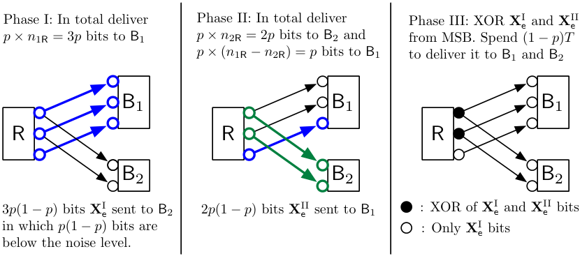
Fig. 3: Example for achieving corner point (17) with (n1​𝖱,n2​𝖱)=(3,2)(n_{1\mathsf{R}},n_{2\mathsf{R}})=(3,2) for the binary expansion downlink with delayed state information

In this subsection, we employ a binary expansion model corresponding to the downlink phase (1) to obtain insights. In this model, the transmitted and received signals are binary vectors in 𝔽2q\mathbb{F}_{2}^{q}, where 𝔽2\mathbb{F}_{2} denotes the binary field {0,1}\{0,1\}. The received signals are Y𝖡i[t]=𝐇𝖡i​𝖱Si[t]X𝖱[t],i=1,2,Y_{\mathsf{B}_{i}}[t]=\mathbf{H}_{\mathsf{B}_{i}\mathsf{R}}S_{i}[t]X_{\mathsf{R}}[t],\ i=1,2, where additions are modulo-two component-wise. Channel transfer matrices are defined as follows: for i=1,2i=1,2, 𝐇𝖡i​𝖱:=𝐒q−ni​𝖱\mathbf{H}_{\mathsf{B}_{i}\mathsf{R}}:=\mathbf{S}^{q-n_{i\mathsf{R}}} where q=maxi=1,2⁡{ni​𝖱}q=\max_{i=1,2}\left\{n_{i\mathsf{R}}\right\} and 𝐒∈𝔽2q×q\mathbf{S}\in\mathbb{F}_{2}^{q\times q} is the shift matrix defined in [5]. The corner point corresponds to (15) and (16) in this model is

(R1,R2)=(p⁡(n1​𝖱−n2​𝖱)+p⁡(2−p)3−p​n2​𝖱,p⁡(2−p)3−p​n2​𝖱).\textstyle(R_{1},R_{2})=\left(p(n_{1\mathsf{R}}-n_{2\mathsf{R}})+\frac{p(2-p)}{3-p}n_{2\mathsf{R}},\frac{p(2-p)}{3-p}n_{2\mathsf{R}}\right). (17)

To achieve this point, the relay uses a three-phase coding scheme extending that in [11]. In Phases I and II (each with block length TT), the relay sends bits intended for 𝖡1\mathsf{B}_{1} and 𝖡2\mathsf{B}_{2}, using the top n1​𝖱n_{1\mathsf{R}} and n2​𝖱n_{2\mathsf{R}} levels respectively. In addition, in Phase II the relay also uses the bottom (n1​𝖱−n2​𝖱)\left(n_{1\mathsf{R}}-n_{2\mathsf{R}}\right) levels to deliver additional bits to 𝖡1\mathsf{B}_{1}. Hence, 𝖡1\mathsf{B}_{1} and 𝖡2\mathsf{B}_{2} receive roughly T​p​(n1​𝖱+n1​𝖱−n2​𝖱)Tp\left(n_{1\mathsf{R}}+n_{1\mathsf{R}}-n_{2\mathsf{R}}\right) and T​p​n2​𝖱Tpn_{2\mathsf{R}} desired bits in Phase I and II respectively.

In Phase I, there will be roughly T​p​(1−p)​n1​𝖱Tp(1-p)n_{1\mathsf{R}} bits which are erased at 𝖡1\mathsf{B}_{1} but erroneously sent to 𝖡2\mathsf{B}_{2} can be used as side-information. We denote this length-T​p​(1−p)Tp(1-p) sequence of n1​𝖱n_{1\mathsf{R}}-level binary vector by 𝐗𝖾I\mathbf{X}_{\mathsf{e}}^{\mathrm{I}}. Note that the bottom (n1​𝖱−n2​𝖱)\left(n_{1\mathsf{R}}-n_{2\mathsf{R}}\right) levels will lie below the noise level at 𝖡2\mathsf{B}_{2} and will NOT appear in this binary expansion model. Similarly in Phase II, there will be such a length T​p​(1−p)Tp(1-p) sequence of n2​𝖱n_{2\mathsf{R}}-level binary vector intended for 𝖡2\mathsf{B}_{2} but only received by 𝖡1\mathsf{B}_{1}. We denote it by 𝐗𝖾II\mathbf{X}_{\mathsf{e}}^{\mathrm{II}}. We aim to recycle these bits in Phase III.

The block length of Phase III is roughly T​p​(1−p)Tp(1-p). In Phase III, the relay makes use of delayed state information to form 𝐗𝖾I\mathbf{X}_{\mathsf{e}}^{\mathrm{I}} and 𝐗𝖾II\mathbf{X}_{\mathsf{e}}^{\mathrm{II}}. Then it sends out 𝐗𝖾I⊕𝐗𝖾II\mathbf{X}_{\mathsf{e}}^{\mathrm{I}}\oplus\mathbf{X}_{\mathsf{e}}^{\mathrm{II}} from the MSB level as depicted on the rightmost of Figure 3. Hence the bottom (n1​𝖱−n2​𝖱)\left(n_{1\mathsf{R}}-n_{2\mathsf{R}}\right) levels consists of bits in the bottom levels of 𝐗𝖾I\mathbf{X}_{\mathsf{e}}^{\mathrm{I}} only. With side information received in Phase I and II, each receiver can decode the desired bits from the received XORs. In total the numbers of bits recycled in this phase are T​p​(1−p)​n1​𝖱Tp(1-p)n_{1\mathsf{R}} and T​p​(1−p)​n2​𝖱Tp(1-p)n_{2\mathsf{R}} at 𝖡1\mathsf{B}_{1} and 𝖡2\mathsf{B}_{2} respectively.

Putting everything together, we achieve R2=p⁡(2−p)3−p​n2​𝖱R_{2}=\frac{p(2-p)}{3-p}n_{2\mathsf{R}} and R1=p⁡{(3−p)​n1​𝖱−n2​𝖱}3−p=p⁡(n1​𝖱−n2​𝖱)+p⁡(2−p)3−p​n2​𝖱R_{1}=\frac{p\left\{(3-p)n_{1\mathsf{R}}-n_{2\mathsf{R}}\right\}}{3-p}=p(n_{1\mathsf{R}}-n_{2\mathsf{R}})+\frac{p(2-p)}{3-p}n_{2\mathsf{R}}.

V-B Proof Sketch of Bounded-gap Achievement to the Corner Point (15) (16) of the Outer Bound Region

Extending to the Gaussian case, we face the following two challenges. First, in Gaussian channel, we are sending complex symbols instead of binary bits and there will be additive Gaussian noise. Second, we need to incorporate superposition coding into Phase II of Fig. 3, while 𝖡1\mathsf{B}_{1} may not be able to decode and cancel the higher-layer codeword since the erasure state process at 𝖡1\mathsf{B}_{1} and 𝖡2\mathsf{B}_{2} are different. Note that only signals of 𝖡2\mathsf{B}_{2} in Phase II have recycling from Phase III.

We solve the first challenge by resending erased symbols instead of bits in the third phase. To do this, the relay will quantize the sum sequence formed by the erased symbols, X𝖾I+X𝖾IIX_{\mathsf{e}}^{\mathrm{I}}+X_{\mathsf{e}}^{\mathrm{II}}, and then send out the quantization indices. Based on the insight learned in the binary expansion model, we know that the resolution of reconstruction must be different: 𝖡1\mathsf{B}_{1} requires higher resolution than 𝖡2\mathsf{B}_{2} since X𝖾IX_{\mathsf{e}}^{\mathrm{I}} goes deeper in the bit levels. Hence, instead of directly quantizing into a single quantization index, we employ successive refinement source coding [15] so that 𝖡1\mathsf{B}_{1} is able to get a higher resolution in reconstruction. Again gaining insights from the binary expansion model, since the number of layers used by 𝖡i\mathsf{B}_{i} is ni​𝖱n_{i\mathsf{R}} for i=1,2i=1,2 in Phase I and II respectively, the MSE of the reconstruction at 𝖡i\mathsf{B}_{i} should be inverse proportional to 𝖲𝖭𝖱i​𝖱,i=1,2\mathsf{SNR}_{i\mathsf{R}},i=1,2.

For the second challenge, we aim to solve it using dirty paper coding (DPC). However, the conventional DPC requires fully known channel information S1​(t)​h𝖡1​𝖱S_{1}(t)h_{\mathsf{B}_{1}\mathsf{R}} at the transmitter [14]. In our case, the current on/off state S1​(t)S_{1}(t) is unknown at the relay. Hence, we propose new one-dimensional (symbol-based) lattice strategy to solve this problem.

Our scheme is summarized as follows
Phase I: By using random Gaussian codebook, relay sends coded symbols X𝖱​[t]X_{\mathsf{R}}[t], t=1​…​Tt=1\ldots T from the codeword representing message for user 𝖡1\mathsf{B}_{1}.

Phase II: Relay sends X𝖱​[t]=X2​𝖱​[t]+X1​𝖱​[t]X_{\mathsf{R}}[t]=X_{2\mathsf{R}}[t]+X_{1\mathsf{R}}[t], t=T+1​…​2​Tt=T+1\ldots 2T, where X2​𝖱​[t]X_{2\mathsf{R}}[t] are coded symbols for user 𝖡2\mathsf{B}_{2} and

X1​𝖱​[t]=(C1​𝖱​[t]−w⋅h𝖡1​𝖱​X2​𝖱​[t]−d⁡[t])modLX_{1\mathsf{R}}[t]=\left(C_{1\mathsf{R}}[t]-w\cdot h_{\mathsf{B}_{1}\mathsf{R}}X_{2\mathsf{R}}[t]-d[t]\right)\mod\;L (18)

where similar to (14), C1​𝖱​[t]C_{1\mathsf{R}}[t] is coded symbol for user 𝖡1\mathsf{B}_{1}. d⁡[t]d[t] is the independent dither. For a real number x,xmodL=x−QL​(x)x,x\mod\;L=x-Q_{L}(x) with QL​(x)Q_{L}(x) being the nearest multiple of LL to xx.

Phase III: Let the erased symbols sent to the wrong receiver in Phase 1 and 2 be X𝖾IX^{\mathrm{I}}_{\mathsf{e}} and X𝖾IIX^{\mathrm{II}}_{\mathsf{e}} respectively. Relay first quantizes the length T​p​(1−p)Tp(1-p) sequence X𝖾I+X𝖾IIX^{\mathrm{I}}_{\mathsf{e}}+X^{\mathrm{II}}_{\mathsf{e}} using successive refinement into indexes i𝖼i_{\mathsf{c}} and i𝗋i_{\mathsf{r}}, where i𝖼i_{\mathsf{c}} is the common index which will be decoded for both 𝖡1\mathsf{B}_{1} and 𝖡2\mathsf{B}_{2} while i𝗋i_{\mathsf{r}} is the refinement index which will be decoded only at 𝖡1\mathsf{B}_{1}. Gaussian superposition channel coding with length T⁡(1−p)T(1-p) is adopted to transmit (i𝖼CLOSE(i_{\mathsf{c}},OPENi𝗋)i_{\mathsf{r}}).

Now, user 𝖡2\mathsf{B}_{2} can know the noisy reconstruction X𝖾I+X𝖾II+Z𝖣​2X^{\mathrm{I}}_{\mathsf{e}}+X^{\mathrm{II}}_{\mathsf{e}}+Z_{\mathsf{D}2} with MSE 𝖣2\mathsf{D}_{2}, by decoding i𝖼i_{\mathsf{c}}. With proper power allocation, 𝖡1\mathsf{B}_{1} (better channel) knows the reconstruction X𝖾I+X𝖾II+Z𝖣​1X^{\mathrm{I}}_{\mathsf{e}}+X^{\mathrm{II}}_{\mathsf{e}}+Z_{\mathsf{D}1} by successively decoding i𝖼i_{\mathsf{c}} and i𝗋i_{\mathsf{r}}, where reconstruction error Z𝖣​1Z_{\mathsf{D}1} has smaller MSE 𝖣1\mathsf{D}_{1} than that of Z𝖣​2Z_{\mathsf{D}2}. For this two-receiver source-channel coding, the rates for common index i𝖼i_{\mathsf{c}} and refinement index i𝗋i_{\mathsf{r}} are chosen as

log⁡(1+2𝖣2)​and​log⁡(1+2𝖣1)−log⁡(1+2𝖣2)\textstyle\log\left(1+\frac{2}{\mathsf{D}_{2}}\right)\ \text{and}\ \textstyle\log\left(1+\frac{2}{\mathsf{D}_{1}}\right)-\log\left(1+\frac{2}{\mathsf{D}_{2}}\right) (19)

respectively. To ensure successful channel decoding at receivers, we need to carefully choosing the power allocation of the superposition channel coding, as well as 𝖣1\mathsf{D}_{1} and 𝖣2\mathsf{D}_{2} in (19). Let the power allocation for indexes i𝖼i_{\mathsf{c}} and i𝗋i_{\mathsf{r}} be 𝖲𝖭𝖱𝖼\mathsf{SNR_{c}} and 𝖲𝖭𝖱𝗋\mathsf{SNR_{r}} respectively. We choose 𝖲𝖭𝖱𝗋=1/𝖲𝖭𝖱𝟤​𝖱,𝖲𝖭𝖱𝖼=𝟣−𝖲𝖭𝖱𝗋\mathsf{SNR_{r}}=1/\mathsf{SNR_{2R}},\mathsf{SNR_{c}=1-SNR_{r}}. (Here we only provide the proof when 𝖲𝖭𝖱2​𝖱≥2\mathsf{SNR}_{2\mathsf{R}}\geq 2, since the bounded-gap result for 𝖲𝖭𝖱2​𝖱<2\mathsf{SNR}_{2\mathsf{R}}<2 is trivial.) For 𝖡2\mathsf{B}_{2} to correctly decode i𝖼i_{\mathsf{c}}, from (19) and the lengths of channel and source codes, we need to choose

𝖣2=4𝖲𝖭𝖱𝟤​𝖱−1\textstyle\mathsf{D}_{2}=\frac{4}{\mathsf{SNR_{2R}}-1} (20)

For receiver 𝖡1\mathsf{B}_{1} to decode both i𝖼i_{\mathsf{c}} and i𝗋i_{\mathsf{r}}, we choose

𝖣1=4𝖲𝖭𝖱𝟣​𝖱+𝖲𝖭𝖱𝟤​𝖱.\textstyle\mathsf{D}_{1}=\frac{4}{\mathsf{SNR_{1R}}+\mathsf{SNR_{2R}}}. (21)

Note that 𝖣i\mathsf{D}_{i} is inverse proportional to 𝖲𝖭𝖱i​𝖱,i=1,2\mathsf{SNR}_{i\mathsf{R}},i=1,2, consistent with the insights from the binary expansion model.

Now receivers 𝖡i,i=1,2\mathsf{B}_{i},i=1,2 can obtain reconstructions of erased symbols X𝖾I+X𝖾IIX^{\mathrm{I}}_{\mathsf{e}}+X^{\mathrm{II}}_{\mathsf{e}} with 𝖣𝟣\mathsf{D_{1}} in (21) and 𝖣𝟤\mathsf{D_{2}} in (20) respectively. With side-information X𝖾IX^{\mathrm{I}}_{\mathsf{e}} (noisy) from Phase I, 𝖡2\mathsf{B}_{2} can combine T​p​(1−p)Tp(1-p) reconstructed symbols X𝖾II+Z𝖣​2−Z𝖡2X^{\mathrm{II}}_{\mathsf{e}}+Z_{\mathsf{D}2}-Z_{\mathsf{B}_{2}} and the T​pTp un-erased symbols received in Phase II to decode XOR Σ2\Sigma_{2}. Then (16) is achievable with bounded gap Δ2\Delta_{2}. To see this, we can first upper-bound the MSE distortion 𝖣2\mathsf{D}_{2} in (20) as

𝖣2≤8𝖲𝖭𝖱𝟤​𝖱.\textstyle\mathsf{D}_{2}\leq\frac{8}{\mathsf{SNR_{2R}}}. (22)

By choosing the power allocation of X𝟣​𝖱X_{\mathsf{1R}} and X𝟤​𝖱X_{\mathsf{2R}} in Phase II be 1/𝖲𝖭𝖱𝟤​𝖱1/\mathsf{SNR_{2R}} and 1−1/𝖲𝖭𝖱𝟤​𝖱1-1/\mathsf{SNR_{2R}} respectively, together with the independence of these two signals, we have the following achievable rate for user 𝖡2\mathsf{B}_{2}

R2≥1(3−p)​(CLOSE\displaystyle R_{2}\geq\frac{1}{(3-p)}\Bigg( p⁡(1−p)​𝒞​(1−1𝖲𝖭𝖱𝟤​𝖱8𝖲𝖭𝖱𝟤​𝖱+1𝖲𝖭𝖱𝟤​𝖱+1𝖲𝖭𝖱𝟤​𝖱)\displaystyle p(1-p)\mathcal{C}\bigg(\frac{1-\frac{1}{\mathsf{SNR_{2R}}}}{\frac{8}{\mathsf{SNR_{2R}}}+\frac{1}{\mathsf{SNR_{2R}}}+\frac{1}{\mathsf{SNR_{2R}}}}\bigg)
OPEN+p​𝒞​(1−1𝖲𝖭𝖱𝟤​𝖱1𝖲𝖭𝖱𝟤​𝖱+1𝖲𝖭𝖱𝟤​𝖱))\displaystyle+p\;\mathcal{C}\bigg(\frac{1-\frac{1}{\mathsf{SNR_{2R}}}}{\frac{1}{\mathsf{SNR_{2R}}}+\frac{1}{\mathsf{SNR_{2R}}}}\bigg)\Bigg) (23)

where (22) is applied to obtain the first term in the RHS of (23). Then bounded gap result can be obtained from (23).

Now we show that for user 𝖡1\mathsf{B}_{1}, rate R1−Δ1R_{1}-\Delta_{1}, with R1R_{1} in (15), is achievable. Following similar procedure as 𝖡2\mathsf{B}_{2} aforementioned, by combining the erased symbols with the un-erased symbols received in Phase I, the following rate is achievable to decode XOR Σ1\Sigma_{1},

p⁡(2−p)3−p​𝒞​(𝖲𝖭𝖱𝟣​𝖱)−p⁡(1−p)3−p​log⁡(3).\displaystyle\textstyle\frac{p(2-p)}{3-p}\mathcal{C}(\mathsf{SNR_{1R}})-\frac{p(1-p)}{3-p}\log(3). (24)

where the following inequality from (21) is used

𝖣1≤2𝖲𝖭𝖱𝟣​𝖱.\textstyle\mathsf{D}_{1}\leq\frac{2}{\mathsf{SNR_{1R}}}.

Moreover, user 𝖡​1\mathsf{B}1 can decode additional messages by forming the following channel from the un-erased symbols in Phase II,

[C1​𝖱​[t]+EL​(t)]modL,\displaystyle\left[C_{1\mathsf{R}}[t]+E_{L}(t)\right]\mod\;L, (25)

where EL​(t)=(w​h𝖡𝟣​𝖱−1)​X1​𝖱​[t]+w​Z𝖡𝟣​[t]E_{L}(t)=(wh_{\mathsf{B_{1}R}}-1)X_{1\mathsf{R}}[t]+wZ_{\mathsf{B_{1}}}[t]. The channel (25) is a modulo-LL channel with length T​pTp and power L2/12=1/𝖲𝖭𝖱𝟤​𝖱L^{2}/12=1/\mathsf{SNR_{2R}}, then rate

p3−p​(log⁡(𝖲𝖭𝖱𝟣​𝖱𝖲𝖭𝖱𝟤​𝖱)−log⁡(2​π​e/12))\displaystyle\textstyle\frac{p}{3-p}\left(\log\left(\frac{\mathsf{SNR_{1R}}}{\mathsf{SNR_{2R}}}\right)-\log(2\pi e/12)\right) (26)

is achievable. By summing (26) and (24), our achievable rate for user 𝖡1\mathsf{B}_{1} has bounded gap to (15)

-C Detailed proof of the Inner Bound ℛG,inul​(d)\mathscr{R}^{\mathrm{ul}}_{\mathrm{G},\mathrm{in}}\left(\mathrm{d}\right) in (10)

Here we focus on the bounded-gap achievability to the sum rate in (4) by joint lattice decoding. From (12) and (14), it can be easily shown that the post-processed signal

(𝐖𝐲𝖱+[(𝐝𝖠1+𝐝𝖡1)T​(𝐝𝖠2+𝐝𝖡2)T]T)​mod​(ΛS×ΛS).\left(\mathbf{Wy}_{\mathsf{R}}+[(\mathbf{d}_{\mathsf{A}_{1}}+\mathbf{d}_{\mathsf{B}_{1}})^{T}\;\;(\mathbf{d}_{\mathsf{A}_{2}}+\mathbf{d}_{\mathsf{B}_{2}})^{T}]^{T}\right)\;\mathrm{mod}\;(\Lambda_{S}\times\Lambda_{S}).

equals to

([(𝐜A1+𝐜B1)T​(𝐜A2+𝐜B2)T]T+𝐄)​mod​(ΛS×ΛS),\displaystyle\left(\left[(\mathbf{c}_{A_{1}}+\mathbf{c}_{B_{1}})^{T}\;\;(\mathbf{c}_{A_{2}}+\mathbf{c}_{B_{2}})^{T}\right]^{T}+\mathbf{E}\right)\;\mathrm{mod}\;(\Lambda_{S}\times\Lambda_{S}), (27)

where

𝐄=(𝐖𝐇−𝐈)​[(𝐱𝖠1+𝐱𝖡1)T​(𝐱𝖠2+𝐱𝖡2)T]T+𝐖𝐳𝖱,\mathbf{E}=\left(\mathbf{W}\mathbf{H}-\mathbf{I}\right)\left[(\mathbf{x}_{\mathsf{A}_{1}}+\mathbf{x}_{\mathsf{B}_{1}})^{T}\;\;(\mathbf{x}_{\mathsf{A}_{2}}+\mathbf{x}_{\mathsf{B}_{2}})^{T}\right]^{T}+\mathbf{Wz}_{\mathsf{R}}, (28)

and 𝐇=[𝐇𝖠1​𝐇𝖠2]\mathbf{H}=\left[\mathbf{H}_{\mathsf{A}_{1}}\;\mathbf{H}_{\mathsf{A}_{2}}\right]. Moreover, in (27), the sum of user codewords within a pair i=1,2i=1,2 is still a lattice codeword

(𝐜𝖠​i+𝐜𝖡​i)​mod​ΛS∈Λi.(\mathbf{c}_{\mathsf{A}i}+\mathbf{c}_{\mathsf{B}i})\;\mathrm{mod}\;\Lambda_{S}\in\Lambda_{i}.

Then from [13], the following sum rate is achievable by jointly lattice decoding

R1+R2≥limT→∞12​T​log⁡(|12​𝐈||ΣE|),R_{1}+R_{2}\geq\mathop{\lim}\limits_{T\rightarrow\infty}\frac{1}{2T}\log\left(\frac{|\frac{1}{2}\mathbf{I}|}{|\Sigma_{E}|}\right), (29)

where ΣE\Sigma_{E} is the covariance matrix of 𝐄\mathbf{E} in (28). With 𝐖\mathbf{W} chosen as the MMSE filter, the information lossless property of MMSE estimation can be invoked, then the sum rate in (29) becomes

R1+R2≥limT→∞12​T​log⁡(|12​𝐈+𝐇𝐇T|).R_{1}+R_{2}\geq\mathop{\lim}\limits_{T\rightarrow\infty}\frac{1}{2T}\log\left(\left|\frac{1}{2}\mathbf{I}+\mathbf{H}\mathbf{H}^{T}\right|\right). (30)

Now from (13) (𝐇=[𝐇𝖠1​𝐇𝖠2]\mathbf{H}=\left[\mathbf{H}_{\mathsf{A}_{1}}\;\mathbf{H}_{\mathsf{A}_{2}}\right]) and the ergodicity of state process,

R1+R2≥\displaystyle R_{1}+R_{2}\geq ES1,S2​[𝒞⁡(S1​𝖲𝖭𝖱𝖱𝟣+S2​𝖲𝖭𝖱𝖱𝟤)]−1\displaystyle\mathrm{E}_{S_{1},S_{2}}\left[\mathcal{C}\left(S_{1}\mathsf{SNR_{R1}}+S_{2}\mathsf{SNR_{R2}}\right)\right]-1
≥\displaystyle\geq p⁡(1−p)​(𝒞⁡(𝖲𝖭𝖱𝖱𝟣+𝒞​𝖲𝖭𝖱𝖱𝟤))\displaystyle\;p(1-p)\left(\mathcal{C}\left(\mathsf{SNR_{R1}}+\mathcal{C}\mathsf{SNR_{R2}}\right)\right)
+p2​𝒞​(𝖲𝖭𝖱𝖱𝟣+𝖲𝖭𝖱𝖱𝟤)−1\displaystyle+p^{2}\mathcal{C}\left(\mathsf{SNR_{R1}}+\mathsf{SNR_{R2}}\right)-1 (31)

To compared (31) with (4), it can be easily checked that

𝒞⁡(𝖲𝖭𝖱𝖱𝟣+𝖲𝖭𝖱𝖱𝟤+𝟤​𝖲𝖭𝖱𝖱𝟣​𝖲𝖭𝖱𝖱𝟤)\displaystyle\mathcal{C}\left(\mathsf{SNR_{R1}}+\mathsf{SNR_{R2}+2\sqrt{\mathsf{SNR_{R1}}\mathsf{SNR_{R2}}}}\right)
≤\displaystyle\leq 1+𝒞⁡(𝖲𝖭𝖱𝖱𝟣+𝖲𝖭𝖱𝖱𝟤).\displaystyle 1+\mathcal{C}\left(\mathsf{SNR_{R1}}+\mathsf{SNR_{R2}}\right). (32)

Then the bounded-gap result for sum rate (4) is established. The bounded-gap achievement to the RHSs of (3) follows similarly. As a final note, decoding correct (𝐜𝖠​i+𝐜𝖡​i)​mod​ΛS(\mathbf{c}_{\mathsf{A}i}+\mathbf{c}_{\mathsf{B}i})\;\mathrm{mod}\;\Lambda_{S} from aforementioned joint lattice decoding equals to decode corrects XORs Σi=W𝖠i⊕W𝖡i,i=1,2\Sigma_{i}=W_{\mathsf{A}_{i}}\oplus W_{\mathsf{B}_{i}},i=1,2 [6].

-D Detailed proof of the inner bound ℛG,indl​(d)\mathscr{R}^{\mathrm{dl}}_{\mathrm{G},\mathrm{in}}\left(\mathrm{d}\right) in (10)

Here we provide the detailed proof for achieving the Gaussian downlink rate region with delayed state information ℛG,indl​(d)\mathscr{R}^{\mathrm{dl}}_{\mathrm{G},\mathrm{in}}\left(\mathrm{d}\right). We assume that state (S1t−1,S2t−1)(S_{1}^{t-1},S_{2}^{t-1}) are known at both receivers 𝖡1\mathsf{B}_{1} and 𝖡2\mathsf{B}_{2} at time tt. In the following, we only provide the proof when 𝖲𝖭𝖱2​𝖱≥2\mathsf{SNR}_{2\mathsf{R}}\geq 2, since the bounded-gap result for 𝖲𝖭𝖱2​𝖱<2\mathsf{SNR}_{2\mathsf{R}}<2 is trivial. We first focus on the proposed three-phase scheme to achieve (R1−Δ1,R2−Δ2)(R_{1}-\Delta_{1},R_{2}-\Delta_{2}) from (15)(16), where (Δ1,Δ2)(\Delta_{1},\Delta_{2}) are given in (8)(9). Here we give the detailed definitions of the erased symbol sequences X𝖾𝖨X^{\mathsf{I}}_{\mathsf{e}} and X𝖾𝖨𝖨X^{\mathsf{II}}_{\mathsf{e}} in Phase III. First, the X𝖱​[t]X_{\mathsf{R}}[t], t=1​…​Tt=1\ldots T in Phase I forms a codeword from a random Gaussian codebook to encode Σ1\Sigma_{1} for 𝖡1\mathsf{B}_{1}. In Phase III, from the delayed state information, the relay knows the erased indexes tts where state sequence with length T1T_{1} of which (S1​[t],S2​[t])=(0,1)(S_{1}[t],S_{2}[t])=(0,1) in Phase I, 1≤t≤T1\leq t\leq T. For each X𝖱​[t]X_{\mathsf{R}}[t], we assign it to an unique symbol X𝖾𝖨​[t′]=X𝖱​[t]X^{\mathsf{I}}_{\mathsf{e}}[t^{\prime}]=X_{\mathsf{R}}[t] in the erased symbol sequence. If T1>T​p​(1−p)T_{1}>Tp(1-p), then we abandon the last T1−T​p​(1−p)T_{1}-Tp(1-p) symbols. On the contrary, if T1<T​p​(1−p)T_{1}<Tp(1-p), we set X𝖾𝖨[t′]=0,t′=T1+1,…Tp(1−p)X_{\mathsf{e}}^{\mathsf{I}}[t^{\prime}]=0,t^{\prime}=T_{1}+1,\ldots Tp(1-p). Then the total length of erased symbol sequence X𝖾𝖨​[t′]X_{\mathsf{e}}^{\mathsf{I}}[t^{\prime}] in Phase I is T​p​(1−p)Tp(1-p). B1B_{1} also knows the mapping from tt to t′t^{\prime} as Π𝖨\Pi_{\mathsf{I}}, where t=Π𝖨​(t′)t=\Pi_{\mathsf{I}}(t^{\prime}) with t′=1​…​min⁡{T1,T​p​(1−p)},1≤t≤Tt^{\prime}=1\ldots\min\{T_{1},Tp(1-p)\},1\leq t\leq T. The mapping Π𝖨\Pi_{\mathsf{I}} is also known at receiver 𝖡1\mathsf{B}_{1}. In Phase II, X2​𝖱​[t]X_{2\mathsf{R}}[t], t=T+1,…,2​Tt=T+1,\ldots,2T (independent of X1​𝖱​[t]X_{1\mathsf{R}}[t] in (18)) forms a codeword from a Gaussian codebook to encode Σ2\Sigma_{2} for 𝖡2\mathsf{B}_{2}. And as aforementioned, we can form length T​p​(1−p)Tp(1-p) erased symbol sequence in Phase II X𝖾𝖨𝖨​[Π𝖨𝖨​(t′)]=X1​𝖱​[t]+X2​𝖱​[t]X_{\mathsf{e}}^{\mathsf{II}}[\Pi_{\mathsf{II}}(t^{\prime})]=X_{1\mathsf{R}}[t]+X_{2\mathsf{R}}[t] from the state sequence with length T2T_{2} of which (S1​[t],S2​[t])=(1,0)(S_{1}[t],S_{2}[t])=(1,0), T+1≤t≤2​TT+1\leq t\leq 2T. The corresponding mapping Π𝖨𝖨\Pi_{\mathsf{II}} is known at receiver 𝖡2\mathsf{B}_{2}.

In Phase III, the relay compresses the sum of erased symbol sequence X𝖾𝖨​[t′]+X𝖾𝖨𝖨​[t′],t′=1​…​T​p​(1−p)X_{\mathsf{e}}^{\mathsf{I}}[t^{\prime}]+X_{\mathsf{e}}^{\mathsf{II}}[t^{\prime}],t^{\prime}=1\ldots Tp(1-p) with successive refinement, and send the corresponding quantization indexes i𝖼i_{\mathsf{c}} and i𝗋i_{\mathsf{r}} through the on/off downlink. At receiver 𝖡i,i=1,2\mathsf{B}_{i},i=1,2, with successfully decoding the quantization index(es), we wish to obtain the following reconstruction

X𝖾𝖨​[t′]+X𝖾𝖨𝖨​[t′]+Z𝖣​i​[t′]X_{\mathsf{e}}^{\mathsf{I}}[t^{\prime}]+X_{\mathsf{e}}^{\mathsf{II}}[t^{\prime}]+Z_{\mathsf{D}i}[t^{\prime}] (33)

where Z𝖣​i∼𝒞​𝒩​(0,𝖣i)Z_{\mathsf{D}i}\sim\mathcal{CN}\left(0,\mathsf{D}_{i}\right) and 𝖣1≤𝖣2\mathsf{D}_{1}\leq\mathsf{D}_{2}. To solve this two-receiver source-channel coding problem, we need to carefully select the lengths and rates of the source and channel codes. The length of source code is T​p​(1−p)Tp(1-p), and the rate selection of the source code comes as follows. To validate (33), we form the following test channels for successive refinement

V1=X𝗌𝗎𝗆+Z;\displaystyle V_{1}=X_{\mathsf{sum}}+Z; (34)
V2=V1+Z′=X𝗌𝗎𝗆+Z+Z′,\displaystyle V_{2}=V_{1}+Z^{\prime}=X_{\mathsf{sum}}+Z+Z^{\prime}, (35)

with source X𝗌𝗎𝗆X_{\mathsf{sum}} having variance 2 and same distribution as X𝖾𝖨​[t′]+X𝖾𝖨𝖨​[t′]X_{\mathsf{e}}^{\mathsf{I}}[t^{\prime}]+X_{\mathsf{e}}^{\mathsf{II}}[t^{\prime}]; reconstruction errors Z∼𝒞​𝒩​(0,𝖣1)Z\sim\mathcal{CN}\left(0,\mathsf{D}_{1}\right) and Z′∼𝒞​𝒩​(0,𝖣2−𝖣1)Z^{\prime}\sim\mathcal{CN}\left(0,\mathsf{D}_{2}-\mathsf{D}_{1}\right). Here X𝗌𝗎𝗆,ZX_{\mathsf{sum}},Z and Z′Z^{\prime} are independent. Note that due to the modL\mod L operation in (18), the source X𝗌𝗎𝗆X_{\mathsf{sum}} is not Gaussian. We choose the rate for common index i𝖼i_{\mathsf{c}} from (35) as

log⁡(2+(𝖣2−𝖣1)+𝖣1(𝖣2−𝖣1)+𝖣1)=log⁡(1+2𝖣2)\displaystyle\log\left(\frac{2+(\mathsf{D}_{2}-\mathsf{D}_{1})+\mathsf{D}_{1}}{(\mathsf{D}_{2}-\mathsf{D}_{1})+\mathsf{D}_{1}}\right)=\log\left(1+\frac{2}{\mathsf{D}_{2}}\right)
≥\displaystyle\geq I⁡(X𝗌𝗎𝗆,V2),\displaystyle I(X_{\mathsf{sum}};V_{2}), (36)

where the inequality comes from that Gaussian source is the hardest one to quantize [12]. The rate for refinement index i𝗋i_{\mathsf{r}} is chosen as

log⁡(1+2𝖣11+2𝖣2)≥I⁡(X𝗌𝗎𝗆,V1)−I⁡(X𝗌𝗎𝗆,V2).\log\!\left(\frac{1+\frac{2}{\mathsf{D}_{1}}}{1+\frac{2}{\mathsf{D}_{2}}}\right)\geq I(X_{\mathsf{sum}};V_{1})\!-\!I(X_{\mathsf{sum}};V_{2}). (37)

Note that the RHS is similar to the achievable rate in a Gaussian wiretap channel. Thus from [16], we know that for any source with variance 22, the Gaussian source 𝒞​𝒩​(0,2)\mathcal{CN}(0,2) maximizes the RHS. Note that V2→V1→X𝗌𝗎𝗆V_{2}\rightarrow V_{1}\rightarrow X_{\mathsf{sum}}. By choosing V1V_{1} as the reconstruction distribution at 𝖡1\mathsf{B}_{1} while V2V_{2} as that at 𝖡2\mathsf{B}_{2}, from (34)-(37), the MSE distortion at 𝖡1\mathsf{B}_{1} is 𝖣1\mathsf{D}_{1} while that at 𝖡2\mathsf{B}_{2} is 𝖣2\mathsf{D}_{2} respectively [15].

Now we must ensure that the receiver 𝖡1\mathsf{B}_{1} can correctly decode both i𝖼i_{\mathsf{c}} and i𝗋i_{\mathsf{r}} while receiver 𝖡2\mathsf{B}_{2} can correctly decode i𝖼i_{\mathsf{c}}. This task is done by carefully choosing the length and power allocation of the superposition channel coding, as well as 𝖣1\mathsf{D}_{1} and 𝖣2\mathsf{D}_{2} in (36)(37). First, since the channel has on/off probability pp, it is crucial to choose the length of channel code longer than that of source code, which is T⁡(1−p)T(1-p) for the length T​p​(1−p)Tp(1-p) source code. Now indexes i𝖼i_{\mathsf{c}} and i𝗋i_{\mathsf{r}} are channel encoded using independent Gaussian codebooks with power 𝖲𝖭𝖱𝖼\mathsf{SNR_{c}} and 𝖲𝖭𝖱𝗋\mathsf{SNR_{r}} respectively, with power allocation 𝖲𝖭𝖱𝗋=1/𝖲𝖭𝖱𝟤​𝖱,𝖲𝖭𝖱𝖼=𝟣−𝖲𝖭𝖱𝗋\mathsf{SNR_{r}}=1/\mathsf{SNR_{2R}},\mathsf{SNR_{c}=1-SNR_{r}}. For 𝖡2\mathsf{B}_{2} to correctly decode i𝖼i_{\mathsf{c}}, from (36) and the lengths of channel and source codes, we need

T​p​(1−p)​log⁡(1+2𝖣2)\displaystyle Tp(1-p)\log\left(1+\frac{2}{\mathsf{D}_{2}}\right)
≤\displaystyle\leq T⁡(1−p)⋅p​𝒞​(𝖲𝖭𝖱𝟤​𝖱​(1−1𝖲𝖭𝖱𝟤​𝖱)𝖲𝖭𝖱𝟤​𝖱​1𝖲𝖭𝖱𝟤​𝖱+1),\displaystyle T(1-p)\cdot p\;\mathcal{C}\left(\frac{\mathsf{SNR_{2R}}\left(1-\frac{1}{\mathsf{SNR_{2R}}}\right)}{\mathsf{SNR_{2R}}\frac{1}{\mathsf{SNR_{2R}}}+1}\right),

which results in

log⁡(1+2𝖣2)≤log⁡(1+𝖲𝖭𝖱𝟤​𝖱2).\log\left(1+\frac{2}{\mathsf{D}_{2}}\right)\leq\log\left(\frac{1+\mathsf{SNR_{2R}}}{2}\right). (38)

Then we can choose

𝖣2=4𝖲𝖭𝖱𝟤​𝖱−1\mathsf{D}_{2}=\frac{4}{\mathsf{SNR_{2R}}-1} (39)

For receiver 𝖡1\mathsf{B}_{1}, first note that since 𝖲𝖭𝖱𝟣​𝖱≥𝖲𝖭𝖱𝟤​𝖱\mathsf{SNR_{1R}}\geq\mathsf{SNR_{2R}}, then 𝖡1\mathsf{B}_{1} can also successfully decode common index i𝖼i_{\mathsf{c}} by treating the codeword for i𝗋i_{\mathsf{r}} as noise. After subtracting the codewords corresponding to i𝖼i_{\mathsf{c}}, from (37) and the lengths of channel and source codes, we need

log⁡(1+2𝖣1)−log⁡(1+2𝖣2)≤𝒞⁡(𝖲𝖭𝖱𝟣​𝖱𝖲𝖭𝖱𝟤​𝖱)\log\left(1+\frac{2}{\mathsf{D}_{1}}\right)-\log\left(1+\frac{2}{\mathsf{D}_{2}}\right)\leq\mathcal{C}\left(\frac{\mathsf{SNR_{1R}}}{\mathsf{SNR_{2R}}}\right) (40)

to correctly decode refinement index i𝗋i_{\mathsf{r}}. From (39), we must choose 𝖣1\mathsf{D}_{1} satisfying

log⁡(1+2𝖣1)≤log⁡(1+𝖲𝖭𝖱𝟤​𝖱2)+log⁡(1+𝖲𝖭𝖱𝟣​𝖱𝖲𝖭𝖱𝟤​𝖱),\log\left(1+\frac{2}{\mathsf{D}_{1}}\right)\leq\log\left(\frac{1+\mathsf{SNR_{2R}}}{2}\right)+\log\left(1+\frac{\mathsf{SNR_{1R}}}{\mathsf{SNR_{2R}}}\right),

which is equivalent to

1+2𝖣1≤12​(1+𝖲𝖭𝖱𝟣​𝖱𝖲𝖭𝖱𝟤​𝖱+𝖲𝖭𝖱𝟤​𝖱+𝖲𝖭𝖱𝟣​𝖱).1+\frac{2}{\mathsf{D}_{1}}\leq\frac{1}{2}\left(1+\frac{\mathsf{SNR_{1R}}}{\mathsf{SNR_{2R}}}+\mathsf{SNR_{2R}}+\mathsf{SNR_{1R}}\right).

Because 𝖲𝖭𝖱𝟣​𝖱/𝖲𝖭𝖱𝟤​𝖱≥1\mathsf{SNR_{1R}}/\mathsf{SNR_{2R}}\geq 1, the above inequality can be meet if

𝖣1=4𝖲𝖭𝖱𝟣​𝖱+𝖲𝖭𝖱𝟤​𝖱\mathsf{D}_{1}=\frac{4}{\mathsf{SNR_{1R}}+\mathsf{SNR_{2R}}} (41)

Now receivers 𝖡i,i=1,2\mathsf{B}_{i},i=1,2 can obtain reconstructions (33) with 𝖣𝟣\mathsf{D_{1}} in (41) and 𝖣𝟤\mathsf{D_{2}} in (39) respectively, where 𝖣𝟣\mathsf{D_{1}} in (39) is smaller than 𝖣𝟤\mathsf{D_{2}} in (39). Note that the (noisy) erased sequence in Phase I X𝖾𝖨​[t′]X_{\mathsf{e}}^{\mathsf{I}}[t^{\prime}] is known at 𝖡2\mathsf{B}_{2}. As a side-information, 𝖡2\mathsf{B}_{2} can subtract X𝖾𝖨​[t′]X_{\mathsf{e}}^{\mathsf{I}}[t^{\prime}] from reconstructions (33) and obtain X𝖾𝖨𝖨​[t′]+Z𝖣​2​[t′]X_{\mathsf{e}}^{\mathsf{II}}[t^{\prime}]+Z_{\mathsf{D}2}[t^{\prime}] (with additional channel noise). Now 𝖡2\mathsf{B}_{2} can combine the erased X𝖾𝖨𝖨​[t′]+Z𝖣​2​[t′]X_{\mathsf{e}}^{\mathsf{II}}[t^{\prime}]+Z_{\mathsf{D}2}[t^{\prime}] with the un-erased symbols received in Phase II to decode XOR Σ2\Sigma_{2}, with bounded gap to (16) as

R2≥p⁡(2−p)3−p​𝒞​(𝖲𝖭𝖱𝟤​𝖱)−p⁡(1−p)3−p​log⁡(10)−p3−p.\displaystyle R_{2}\geq\frac{p(2-p)}{3-p}\mathcal{C}(\mathsf{SNR_{2R}})-\frac{p(1-p)}{3-p}\log(10)-\frac{p}{3-p}. (42)

The details come as follows. First, we can upper-bound the MSE distortion 𝖣2\mathsf{D}_{2} in (39) as

𝖣2=4𝖲𝖭𝖱𝟤​𝖱−1≤412​𝖲𝖭𝖱𝟤​𝖱=8𝖲𝖭𝖱𝟤​𝖱.\mathsf{D}_{2}=\frac{4}{\mathsf{SNR_{2R}}-1}\leq\frac{4}{\frac{1}{2}\mathsf{SNR_{2R}}}=\frac{8}{\mathsf{SNR_{2R}}}. (43)

The above inequality is due to that the SNR regime we considered 𝖲𝖭𝖱𝟤​𝖱≥2\mathsf{SNR_{2R}}\geq 2 is equivalent to 𝖲𝖭𝖱𝟤​𝖱−1≥12​𝖲𝖭𝖱𝟤​𝖱\mathsf{SNR_{2R}}-1\geq\frac{1}{2}\mathsf{SNR_{2R}}. And from test channel (35), it is ensured that the quantization noise Z𝖣​2​[t′]Z_{\mathsf{D}2}[t^{\prime}] is independent of X𝖾𝖨𝖨​[t′]X_{\mathsf{e}}^{\mathsf{II}}[t^{\prime}]. Now we can from the following sequence to decode Σ2\Sigma_{2} at receiver 𝖡2\mathsf{B}_{2}

Y~𝖡2​[t]={X𝖱​[Π𝖨𝖨−1​(t′)]+Z𝖣2​[Π𝖨𝖨−1​(t′)]−Z𝖡𝟤​[t]h𝖡𝟤​𝖱t=Π𝖨𝖨​(t′)S2​[t]​h𝖡𝟤​𝖱​X𝖱​[t]+Z𝖡𝟤​[t]other​t,\tilde{Y}_{\mathsf{B}_{2}}[t]\!=\!\left\{\!\begin{array}[]{ll}X_{\mathsf{R}}[\Pi_{\mathsf{II}}^{-1}(t^{\prime})]+Z_{\mathsf{D}_{2}}[\Pi^{-1}_{\mathsf{II}}(t^{\prime})]-\frac{Z_{\mathsf{B_{2}}}[t]}{h_{\mathsf{B_{2}R}}}&t=\Pi_{\mathsf{II}}(t^{\prime})\\ S_{2}[t]h_{\mathsf{B_{2}R}}X_{\mathsf{R}}[t]+Z_{\mathsf{B_{2}}}[t]&\mbox{other}\;t,\end{array}\right.

where X𝖱​[t]=X𝟤​𝖱​[t]+X𝟣​𝖱​[t]X_{\mathsf{R}}[t]=X_{\mathsf{2R}}[t]+X_{\mathsf{1R}}[t] with X𝟤​𝖱​[t]X_{\mathsf{2R}}[t] carrying message Σ2\Sigma_{2} and interference X𝟣​𝖱​[t]X_{\mathsf{1R}}[t] from (18), T+1≤t≤2​TT+1\leq t\leq 2T, t′=1​…​min⁡{T1,T2,T​p​(1−p)}t^{\prime}=1\ldots\min\{T_{1},T_{2},Tp(1-p)\}. Note that when T→∞T\rightarrow\infty, T1/T,T2/T→p⁡(1−p)T_{1}/T,T_{2}/T\rightarrow p(1-p) almost surely from our random state process. The power allocations of X𝟣​𝖱X_{\mathsf{1R}} and X𝟤​𝖱X_{\mathsf{2R}} are 1/𝖲𝖭𝖱𝟤​𝖱1/\mathsf{SNR_{2R}} and 1−1/𝖲𝖭𝖱𝟤​𝖱1-1/\mathsf{SNR_{2R}}. When T→∞T\rightarrow\infty, from the independence of X𝟤​𝖱​[t]X_{\mathsf{2R}}[t] and X𝟣​𝖱​[t]X_{\mathsf{1R}}[t] and our power allocation, we have the following achievable rate for user 𝖡2\mathsf{B}_{2}

R2≥1(3−p)​(CLOSE\displaystyle R_{2}\geq\frac{1}{(3-p)}\Bigg( p⁡(1−p)​𝒞​(1−1𝖲𝖭𝖱𝟤​𝖱8𝖲𝖭𝖱𝟤​𝖱+1𝖲𝖭𝖱𝟤​𝖱+1𝖲𝖭𝖱𝟤​𝖱)\displaystyle p(1-p)\mathcal{C}\bigg(\frac{1-\frac{1}{\mathsf{SNR_{2R}}}}{\frac{8}{\mathsf{SNR_{2R}}}+\frac{1}{\mathsf{SNR_{2R}}}+\frac{1}{\mathsf{SNR_{2R}}}}\bigg)
OPEN+p​𝒞​(1−1𝖲𝖭𝖱𝟤​𝖱1𝖲𝖭𝖱𝟤​𝖱+1𝖲𝖭𝖱𝟤​𝖱))\displaystyle+p\;\mathcal{C}\bigg(\frac{1-\frac{1}{\mathsf{SNR_{2R}}}}{\frac{1}{\mathsf{SNR_{2R}}}+\frac{1}{\mathsf{SNR_{2R}}}}\bigg)\Bigg) (44)

where (44) comes from (43) and the fact that Gaussian interference is the worst interference under the same power constraint 1/𝖲𝖭𝖱𝟤​𝖱1/\mathsf{SNR_{2R}}. Then (42) can be easily obtained from (44).

Now we show that for user 𝖡1\mathsf{B}_{1}, bounded-gap rate R1−Δ1R_{1}-\Delta_{1} with R1R_{1} in (15) and Δ1\Delta_{1} in (8), is achievable. Following similar procedure as 𝖡2\mathsf{B}_{2} aforementioned, by combining the erased symbols with the un-erased symbols received in Phase I, the following rate is achievable to decode XOR Σ1\Sigma_{1},

1(3−p)​(p⁡(1−p)​𝒞​(12𝖲𝖭𝖱𝟣​𝖱+1𝖲𝖭𝖱𝟣​𝖱)+p​𝒞​(𝖲𝖭𝖱𝟣​𝖱))\displaystyle\frac{1}{(3-p)}\left(p(1-p)\mathcal{C}\left(\frac{1}{\frac{2}{\mathsf{SNR_{1R}}}+\frac{1}{\mathsf{SNR_{1R}}}}\right)+p\;\mathcal{C}(\mathsf{SNR_{1R}})\right) (45)
≥\displaystyle\geq p⁡(2−p)3−p​𝒞​(𝖲𝖭𝖱𝟣​𝖱)−p⁡(1−p)3−p​log⁡(3).\displaystyle\frac{p(2-p)}{3-p}\mathcal{C}(\mathsf{SNR_{1R}})-\frac{p(1-p)}{3-p}\log(3). (46)

where the following inequality (from (41)) is used for obtaining (45)

𝖣1=4𝖲𝖭𝖱𝟣​𝖱+𝖲𝖭𝖱𝟤​𝖱≤2𝖲𝖭𝖱𝟣​𝖱,\mathsf{D}_{1}=\frac{4}{\mathsf{SNR_{1R}}+\mathsf{SNR_{2R}}}\leq\frac{2}{\mathsf{SNR_{1R}}},

which follows from the assumption 𝖲𝖭𝖱𝟣​𝖱≥𝖲𝖭𝖱𝟤​𝖱\mathsf{SNR_{1R}}\geq\mathsf{SNR_{2R}}. Moreover, user 𝖡​1\mathsf{B}1 can decode additional messages by forming the following channel from the un-erased symbols in Phase II,

{w⁡[h𝖡𝟣​𝖱​(X1​𝖱​[t]+X2​𝖱​[t])+Z𝖡𝟣​[t]]+d⁡(t)}modL\displaystyle\left\{w\left[h_{\mathsf{B_{1}R}}\left(X_{1\mathsf{R}}[t]+X_{2\mathsf{R}}[t]\right)+Z_{\mathsf{B_{1}}}[t]\right]+d(t)\right\}\mod\;L
=\displaystyle= [C1​𝖱​[t]+EL​(t)]modL,\displaystyle\left[C_{1\mathsf{R}}[t]+E_{L}(t)\right]\mod\;L, (47)

where EL​(t)=(w​h𝖡𝟣​𝖱−1)​X1​𝖱​[t]+w​Z𝖡𝟣​[t]E_{L}(t)=(wh_{\mathsf{B_{1}R}}-1)X_{1\mathsf{R}}[t]+wZ_{\mathsf{B_{1}}}[t]. The channel (47) is a modulo-LL channel with length T​pTp and power L2/12=1/𝖲𝖭𝖱𝟤​𝖱L^{2}/12=1/\mathsf{SNR_{2R}}. By choosing ww as the MMSE coefficient, rate

p3−p​(log⁡(𝖲𝖭𝖱𝟣​𝖱𝖲𝖭𝖱𝟤​𝖱)−log⁡(2​π​e/12))\displaystyle\frac{p}{3-p}\left(\log\left(\frac{\mathsf{SNR_{1R}}}{\mathsf{SNR_{2R}}}\right)-\log(2\pi e/12)\right) (48)

is achievable [14]. To compare with (15), note that the RHS of (15) can be rewritten as

13−p​(p⁡(𝒞⁡(𝖲𝖭𝖱𝟣​𝖱)−𝒞⁡(𝖲𝖭𝖱𝟤​𝖱))+p⁡(2−p)​𝒞​(𝖲𝖭𝖱𝟣​𝖱))\displaystyle\frac{1}{3-p}\left(p\left(\mathcal{C}\left(\mathsf{SNR_{1R}}\right)-\mathcal{C}\left(\mathsf{SNR_{2R}}\right)\right)+p(2-p)\mathcal{C}\left(\mathsf{SNR_{1R}}\right)\right)
≤\displaystyle\leq 13−p​(p​log⁡(𝖲𝖭𝖱𝟣​𝖱𝖲𝖭𝖱𝟤​𝖱)+p⁡(2−p)​𝒞​(𝖲𝖭𝖱𝟣​𝖱)),\displaystyle\frac{1}{3-p}\left(p\log\left(\frac{\mathsf{SNR_{1R}}}{\mathsf{SNR_{2R}}}\right)+p(2-p)\mathcal{C}\left(\mathsf{SNR_{1R}}\right)\right), (49)

where the second inequality is due to assumption 𝖲𝖭𝖱𝟣​𝖱≥𝖲𝖭𝖱𝟤​𝖱\mathsf{SNR_{1R}}\geq\mathsf{SNR_{2R}}. By summing (48) and (46), our achievable rate for user 𝖡1\mathsf{B}_{1} has bounded gap to (15) as

R1≥\displaystyle R_{1}\geq p⁡(𝒞⁡(𝖲𝖭𝖱1​𝖱)−𝒞⁡(𝖲𝖭𝖱2​𝖱))+p⁡(2−p)3−p​𝒞​(𝖲𝖭𝖱2​𝖱)\displaystyle p\left(\mathcal{C}(\mathsf{SNR}_{1\mathsf{R}})\!-\!\mathcal{C}(\mathsf{SNR}_{2\mathsf{R}})\right)\!+\!\frac{p(2-p)}{3-p}\mathcal{C}(\mathsf{SNR}_{2\mathsf{R}})
−p⁡(1−p)3−p​log⁡(3)−p3−p​log⁡(2​π​e12).\displaystyle-\frac{p(1-p)}{3-p}\log(3)-\frac{p}{3-p}\log\left(\frac{2\pi e}{12}\right).

Finally, the intersection of (7) and (5) is

(R1,R2)=(p⁡(𝒞⁡(𝖲𝖭𝖱1​𝖱)−𝒞⁡(𝖲𝖭𝖱2​𝖱),p​𝒞​(𝖲𝖭𝖱2​𝖱)CLOSECLOSE.(R_{1},R_{2})=\Big(p\left(\mathcal{C}(\mathsf{SNR}_{1\mathsf{R}})\!-\!\mathcal{C}(\mathsf{SNR}_{2\mathsf{R}}\right),p\mathcal{C}(\mathsf{SNR}_{2\mathsf{R}}\Big). (50)

For this point, we use Gaussian superposition coding to transmit messages Σ1\Sigma_{1} and Σ2\Sigma_{2} with corresponding power allocations 1/𝖲𝖭𝖱𝟤​𝖱1/\mathsf{SNR_{2R}} and 1−1/𝖲𝖭𝖱𝟤​𝖱1-1/\mathsf{SNR_{2R}}. Then we have the following achievable rate pair (R1,R2)(R_{1},R_{2})

(p⁡(𝒞⁡(𝖲𝖭𝖱1​𝖱)−𝒞⁡(𝖲𝖭𝖱2​𝖱),p​𝒞​(𝖲𝖭𝖱2​𝖱)−p)CLOSE,\Big(p\left(\mathcal{C}(\mathsf{SNR}_{1\mathsf{R}})\!-\!\mathcal{C}(\mathsf{SNR}_{2\mathsf{R}}\right),p\mathcal{C}(\mathsf{SNR}_{2\mathsf{R}})-p\Big),

which has bounded gap to (50). And it concludes our proof.

-E Detailed proof of the outer-bound region in (11)

Here we prove that with delayed state information, the region ℛoutdl​(d)\mathscr{R}^{\mathrm{dl}}_{\mathrm{out}}\left(\mathrm{d}\right) defined from (5)(6)(7) is a outer-bound region for the Gaussian model (1)(2). We first focus on (7), which results from first forming an equivalent degraded downlink and then outer-bounding carefully to avoid explicitly selecting the auxiliary random variable UU. Since the noises at receivers in (1) are independent of the delayed state feedback, we can change Y𝖡1Y_{\mathsf{B}_{1}} and Y𝖡2Y_{\mathsf{B}_{2}} as

Y𝖡1=S1​X𝖱+Z𝖡1h𝖡𝟣​𝖱\displaystyle Y_{\mathsf{B}_{1}}=S_{1}X_{\mathsf{R}}+\frac{Z_{\mathsf{B}_{1}}}{h_{\mathsf{B_{1}R}}} (51)
Y𝖡2=S2​X𝖱+Z𝖡2h𝖡𝟤​𝖱=S2​XR+Z𝖡1h𝖡𝟣​𝖱+Z′\displaystyle Y_{\mathsf{B}_{2}}=S_{2}X_{\mathsf{R}}+\frac{Z_{\mathsf{B}_{2}}}{h_{\mathsf{B_{2}R}}}=S_{2}X_{R}+\frac{Z_{\mathsf{B}_{1}}}{h_{\mathsf{B_{1}R}}}+Z^{\prime} (52)

where Z′∼𝒞​𝒩​(0,1𝖲𝖭𝖱2​𝖱−1𝖲𝖭𝖱1​𝖱)Z^{\prime}\sim\mathcal{CN}(0,\frac{1}{\mathsf{SNR}_{2\mathsf{R}}}-\frac{1}{\mathsf{SNR}_{1\mathsf{R}}}). By giving Y𝖡2Y_{\mathsf{B}_{2}} in (52) to 𝖡1\mathsf{B}_{1}, we have physically degraded channel [12] X𝖱→{Y𝖡1,Y𝖡2}→Y𝖡2X_{\mathsf{R}}\rightarrow\{Y_{\mathsf{B}_{1}},Y_{\mathsf{B}_{2}}\}\rightarrow Y_{\mathsf{B}_{2}} with the following outer bounds

R2\displaystyle R_{2} ≤I⁡(U;Y𝖡2|S)\displaystyle\leq I(U;Y_{\mathsf{B}_{2}}|S) (53)
=I(X𝖱,U;Y𝖡2|S2)−I(X𝖱;Y𝖡2|U,S2)\displaystyle=I(X_{\mathsf{R}},U;Y_{\mathsf{B}_{2}}|S_{2})-I(X_{\mathsf{R}};Y_{\mathsf{B}_{2}}|U,S_{2})
=I⁡(X𝖱;Y𝖡2|S2)−p​r\displaystyle=I(X_{\mathsf{R}};Y_{\mathsf{B}_{2}}|S_{2})-pr (54)
=p⋅𝒞⁡(𝖲𝖭𝖱𝟤​𝖱)−p​r,\displaystyle=p\cdot\mathcal{C}(\mathsf{SNR_{2R}})-pr, (55)

where S={S1,S2}S=\{S_{1},S_{2}\} in (53), and (54) comes from conditional Markov Chain U→X𝖱→Y𝖡2U\rightarrow X_{\mathsf{R}}\rightarrow Y_{\mathsf{B}_{2}} given S2S_{2}, and rr is defined as

r≜I(X𝖱;Y𝖡2|U,S2=1);r\triangleq I(X_{\mathsf{R}};Y_{\mathsf{B}_{2}}|U,S_{2}=1); (56)

also

R1≤\displaystyle R_{1}\leq I(X𝖱;Y𝖡1,Y𝖡2|S,U)\displaystyle I(X_{\mathsf{R}};Y_{\mathsf{B}_{1}},Y_{\mathsf{B}_{2}}|S,U)
=\displaystyle= I(X𝖱;Y𝖡1|S,U)+I(X𝖱;Y𝖡2|Y𝖡1,S,U)\displaystyle I(X_{\mathsf{R}};Y_{\mathsf{B}_{1}}|S,U)+I(X_{\mathsf{R}};Y_{\mathsf{B}_{2}}|Y_{\mathsf{B}_{1}},S,U)
=\displaystyle= pI(X𝖱;Y𝖡1|U,S1=1)+p(1−p)I(X𝖱;Y𝖡2|U,S2=1)\displaystyle pI(X_{\mathsf{R}};Y_{\mathsf{B}_{1}}|U,S_{1}=1)+p(1-p)I(X_{\mathsf{R}};Y_{\mathsf{B}_{2}}|U,S_{2}=1)
+p2I(X𝖱;Y𝖡2|Y𝖡1,U,S1=S2=1).\displaystyle+p^{2}I(X_{\mathsf{R}};Y_{\mathsf{B}_{2}}|Y_{\mathsf{B}_{1}},U,S_{1}=S_{2}=1). (57)

From (51) and (52),

I(X𝖱;Y𝖡2|Y𝖡1,U,S1=S2=1)=0,I(X_{\mathsf{R}};Y_{\mathsf{B}_{2}}|Y_{\mathsf{B}_{1}},U,S_{1}=S_{2}=1)=0,

then

R1≤pI(X𝖱;Y𝖡1|U,S1=1)+p(1−p)r\displaystyle R_{1}\leq pI(X_{\mathsf{R}};Y_{\mathsf{B}_{1}}|U,S_{1}=1)+p(1-p)r (58)

With rr defined in (56),

I(X𝖱;Y𝖡1|U,S1=1)−r\displaystyle I(X_{\mathsf{R}};Y_{\mathsf{B}_{1}}|U,S_{1}=1)-r
=\displaystyle= h⁡(X𝖱+Z𝖡1h𝖡𝟣​𝖱|U)−h⁡(Z𝖡1h𝖡𝟣​𝖱)\displaystyle h\left(X_{\mathsf{R}}+\frac{Z_{\mathsf{B}_{1}}}{h_{\mathsf{B_{1}R}}}\Big|U\right)-h\left(\frac{Z_{\mathsf{B}_{1}}}{h_{\mathsf{B_{1}R}}}\right)
−h⁡(X𝖱+Z𝖡2h𝖡𝟤​𝖱|U)+h⁡(Z𝖡2h𝖡𝟤​𝖱)\displaystyle-h\left(X_{\mathsf{R}}+\frac{Z_{\mathsf{B}_{2}}}{h_{\mathsf{B_{2}R}}}\Big|U\right)+h\left(\frac{Z_{\mathsf{B}_{2}}}{h_{\mathsf{B_{2}R}}}\right) (59)
≤\displaystyle\leq 𝒞⁡(𝖲𝖭𝖱1​𝖱)−𝒞⁡(𝖲𝖭𝖱2​𝖱).\displaystyle\mathcal{C}(\mathsf{SNR}_{1\mathsf{R}})-\mathcal{C}(\mathsf{SNR}_{2\mathsf{R}}). (60)

Note that the RHS of (59) is similar to the achievable rate in a Gaussian wiretap channel. From [16] and |h𝖡𝟣​𝖱|≥|h𝖡𝟤​𝖱||h_{\mathsf{B_{1}R}}|\geq|h_{\mathsf{B_{2}R}}|, (60) is valid since the RHS of (59) is maximized when X𝖱X_{\mathsf{R}} is Gaussian conditioned on UU. Substitute (60) into (58), we have

R1\displaystyle R_{1} ≤p⁡(r+𝒞⁡(𝖲𝖭𝖱1​𝖱)−𝒞⁡(𝖲𝖭𝖱2​𝖱))+p⁡(1−p)​r\displaystyle\leq p\left(r+\mathcal{C}(\mathsf{SNR}_{1\mathsf{R}})-\mathcal{C}(\mathsf{SNR}_{2\mathsf{R}})\right)+p(1-p)r
=p⁡(2−p)​r+p⁡(𝒞⁡(𝖲𝖭𝖱1​𝖱)−𝒞⁡(𝖲𝖭𝖱2​𝖱))\displaystyle=p(2-p)r+p\left(\mathcal{C}(\mathsf{SNR}_{1\mathsf{R}})-\mathcal{C}(\mathsf{SNR}_{2\mathsf{R}})\right)

Together with (55), constraint (7) is obtained.

For (6), let us give Y𝖡1Y_{\mathsf{B}_{1}} in (51) to receiver 𝖡2\mathsf{B}_{2}, we have a physically degraded channel X𝖱→{Y𝖡1,Y𝖡2}→Y𝖡1X_{\mathsf{R}}\rightarrow\{Y_{\mathsf{B}_{1}},Y_{\mathsf{B}_{2}}\}\rightarrow Y_{\mathsf{B}_{1}}, and having

R1\displaystyle R_{1} ≤p​𝒞​(𝖲𝖭𝖱𝟣​𝖱)−p​r′,\displaystyle\leq p\;\mathcal{C}(\mathsf{SNR_{1R}})-pr^{\prime}, (61)

where r′=I(X𝖱;Y𝖡1|U,S1=1)r^{\prime}=I(X_{\mathsf{R}};Y_{\mathsf{B}_{1}}|U,S_{1}=1). This inequality follows from steps to reach (55). Also following steps to reach (57)

R2\displaystyle R_{2} ≤pr′+p2I(X𝖱;Y𝖡2|Y𝖡1,U,S1=1,S2=1)\displaystyle\leq pr^{\prime}+p^{2}I(X_{\mathsf{R}};Y_{\mathsf{B}_{2}}|Y_{\mathsf{B}_{1}},U,S_{1}=1,S_{2}=1)
+p(1−p)(X𝖱;Y𝖡2|U,S2=1,S1=0)\displaystyle\;\;\;+p(1-p)(X_{\mathsf{R}};Y_{\mathsf{B}_{2}}|U,S_{2}=1,S_{1}=0)
≤p​r′+p2⋅0+p⁡(1−p)​r′\displaystyle\leq pr^{\prime}+p^{2}\cdot 0+p(1-p)r^{\prime} (62)
=p​r′​(2−p),\displaystyle=pr^{\prime}(2-p), (63)

where (62) comes from the data processing inequality,

I(X𝖱;Y𝖡2|U,S2=1)≤I(X𝖱;Y𝖡1|U,S1=1)=r′,\displaystyle I(X_{\mathsf{R}};Y_{\mathsf{B}_{2}}|U,S_{2}=1)\leq I(X_{\mathsf{R}};Y_{\mathsf{B}_{1}}|U,S_{1}=1)=r^{\prime}, (64)

since given UU and S1=S2=1S_{1}=S_{2}=1, we have the Markov chain X𝖱→Y𝖡1→Y𝖡2X_{\mathsf{R}}\rightarrow Y_{\mathsf{B}_{1}}\rightarrow Y_{\mathsf{B}_{2}} from (51) and (52). From (61) and (63), we have (6), and then ℛoutdl​(d)\mathscr{R}^{\mathrm{dl}}_{\mathrm{out}}\left(\mathrm{d}\right) is a capacity outer bound region. Note that for the binary expansion model in Sec. V-A, by giving Y𝖡2Y_{\mathsf{B}_{2}} to 𝖡1\mathsf{B}_{1}, we get

R1p⁡(2−p)+R2p≤1(2−p)​(n1​𝖱−n2​𝖱)+n2​𝖱.\displaystyle\textstyle\frac{R_{1}}{p(2-p)}+\frac{R_{2}}{p}\leq\textstyle\frac{1}{(2-p)}(n_{1\mathsf{R}}-n_{2\mathsf{R}})+n_{2\mathsf{R}}. (65)

from aforementioned degraded channel arguments. By reversing the role of 𝖡1\mathsf{B}_{1} and 𝖡2\mathsf{B}_{2}, one get

R1p+R2p⁡(2−p)≤n1​𝖱,\displaystyle\textstyle\frac{R_{1}}{p}+\frac{R_{2}}{p(2-p)}\leq n_{1\mathsf{R}}, (66)

And the corner point (17) comes from the intersection of (65) and (66).

The outer-bound region ℛoutul​(d)\mathscr{R}^{\mathrm{ul}}_{\mathrm{out}}\left(\mathrm{d}\right) can be proved by allowing users 𝖠1\mathsf{A}_{1} and 𝖠2\mathsf{A}_{2} cooperate, which is akin to a two transmitter-antennas MISO channel with per antenna power constraint. This concludes our proofs for outer bounds of capacity region with delayed state information 𝒞⁡(d,d)\mathscr{C}(\mathrm{d},\mathrm{d}) in (11).

-F Proof for the rest three regions in Theorem III.1

Now we turn to the bounded-gap result for the capacity region with instantaneous state information for all terminal users and the relay 𝒞G​(i,i)\mathscr{C}_{\mathrm{G}}(\mathrm{i},\mathrm{i}). For (10), to achieve ℛG,inul​(i)\mathscr{R}^{\mathrm{ul}}_{\mathrm{G},\mathrm{in}}\left(\mathrm{i}\right) for the uplink phase, the operations of users and the relay are similar to those for achieving ℛG,inul​(d)\mathscr{R}^{\mathrm{ul}}_{\mathrm{G},\mathrm{in}}\left(\mathrm{d}\right) with delayed state information in Sec IV. The only difference is that one can perform on/off power allocation on (14) with instantaneous state information. In the downlink phase, the region ℛG,indl​(i)\mathscr{R}^{\mathrm{dl}}_{\mathrm{G},\mathrm{in}}\left(\mathrm{i}\right) is fully achievable by Gaussian superposition coding with on/off power allocation. As for the outer-bound regions in (11), the cooperative outer bounds for the uplink with on/off power allocation result in ℛG,outul​(i)\mathscr{R}^{\mathrm{ul}}_{\mathrm{G},\mathrm{out}}\left(\mathrm{i}\right). From the uplink-downlink duality (sum power constraint), ℛG,outdl​(i)\mathscr{R}^{\mathrm{dl}}_{\mathrm{G},\mathrm{out}}\left(\mathrm{i}\right) also a capacity outer-bound region.

Note that in our aforementioned proofs for 𝒞G​(d,d)\mathscr{C}_{\mathrm{G}}(\mathrm{d},\mathrm{d}) and 𝒞G​(i,i)\mathscr{C}_{\mathrm{G}}(\mathrm{i},\mathrm{i}), the capacity outer and inner bounds can be decomposed to those for uplink and downlink. Then these proofs also apply to proving 𝒞G​(i,d)\mathscr{C}_{\mathrm{G}}(\mathrm{i},\mathrm{d}) and 𝒞G​(d,i)\mathscr{C}_{\mathrm{G}}(\mathrm{d},\mathrm{i}), which establishes the bounded-gap results for all four (u,r)(\mathrm{u},\mathrm{r}) combinations in Theorem III.1.

References

  • [1] W. Nam, S.-Y. Chung, and Y. H. Lee, “Capacity of the Gaussian two-way relay channel to within 1/2 bit,” IEEE Transactions on Information Theory, vol. 56, no. 11, pp. 5488–5494, Nov. 2010.
  • [2] A. Sezgin, A. S. Avestimehr, M. A. Khajehnejad, and B. Hassibi, “Divide-and-conquer: Approaching the capacity of the two-pair bidirectional Gaussian relay network,” IEEE Transactions on Information Theory, vol. 58, no. 4, pp. 2434 – 2454, April 2012.
  • [3] A. Osseiran et al., “Scenarios for 5G mobile and wireless communications: the vision of the METIS project,” IEEE Communications Magazine, vol. 52, no. 5, pp. 26–35, May 2014.
  • [4] A. Vahid, M. A. Maddah-Ali, and A. S. Avestimehr, “Approximate capacity of the two-user MISO broadcast channel with delayed CSIT,” in Allerton Conference, Illinois, USA, Oct. 2013, pp. 54–61.
  • [5] A. S. Avestimehr, S. N. Diggavi, and D. N. C. Tse, “Wireless network information flow: a deterministic approach,” IEEE Transactions on Information Theory, vol. 57, no. 4, pp. 1872 – 1905, April 2011.
  • [6] B. Nazer and M. Gastpar, “Compute-and-forward: Harnessing interference through structured codes,” IEEE Transactions on Information Theory, vol. 57, no. 10, pp. 6463–6486, Oct. 2011.
  • [7] I.-H. Wang, C. Suh, S. Diggavi, and P. Viswanath, “Bursty interference channel with feedback,” in IEEE Int. Symp. Inf. Theory (ISIT), 2013.
  • [8] A. Vahid, M. A. Maddah-Ali, and A. S. Avestimehr, “Capacity results for binary fading interference channels with delayed CSIT,” IEEE Transactions on Information Theory, vol. 60, no. 10, pp. 6093–6130, Oct. 2014.
  • [9] S. Hua, C. Geng, and S. A. Jafar, “Topological interference management with alternating connectivity,” in IEEE Int. Symp. Inf. Theory (ISIT), 2013.
  • [10] P. Minero, M. Franceschetti, and D. Tse, “Random access: An information-theoretic perspective,” IEEE Transactions on Information Theory, vol. 58, no. 2, pp. 909–930, Feb. 2012.
  • [11] L. Georgiadis and L. Tassiulas, “Broadcast erasure channel with feedback-capacity and algorithms,” in Proc. Workshop Network Coding, Theory, Appl., Lausanne, Switzerland, Jun. 2009, pp. 54–61.
  • [12] A. El-Gamal and Y.-H. Kim, Network Information Theory. Cambridge University Press, 2011.
  • [13] C.-P. Lee, S.-C. Lin, H.-J. Su, and H. V. Poor, “Multiuser lattice coding for the multiple-access relay channel,” IEEE Transactions on Wireless Communications, vol. 13, no. 7, pp. 3539–3555, Jul. 2014.
  • [14] R. Zamir, S. Shamai, and U. Erez, “Nested linear/lattice codes for structured multiterminal binning,” IEEE Transactions on Information Theory, vol. 48, no. 6, pp. 1250–1276, June 2002.
  • [15] S. Cheng and Z. Xiong, “Successive refinement for the Wyner-Ziv problem and layered code design,” IEEE Transactions on Signal Processing, vol. 53, no. 8, pp. 3269–3281, 2005.
  • [16] S. Leung-Yan-Cheong and M. E. Hellman, “The Gaussian wire-tap channel,” IEEE Transactions on Information Theory, vol. 24, no. 4, pp. 451–456, 1978.