21-cm signal from cosmic dawn - II: Imprints of the light-cone effects
Abstract
Details of various unknown physical processes during the cosmic dawn and the epoch of reionization can be extracted from observations of the redshifted 21-cm signal. These observations, however, will be affected by the evolution of the signal along the line-of-sight which is known as the “light-cone effect”. We model this effect by post-processing a dark matter body simulation with an 1-D radiative transfer code. We find that the effect is much stronger and dramatic in presence of inhomogeneous heating and coupling compared to the case where these processes are not accounted for. One finds increase (decrease) in the spherically averaged power spectrum up to a factor of 3 (0.6) at large scales () when the light-cone effect is included, though these numbers are highly dependent on the source model. The effect is particularly significant near the peak and dip-like features seen in the power spectrum. The peaks and dips are suppressed and thus the power spectrum can be smoothed out to a large extent if the width of the frequency band used in the experiment is large. We argue that it is important to account for the light-cone effect for any 21-cm signal prediction during cosmic dawn.
Keywords:
intergalactic medium - radiative transfer - cosmology: theory - cosmology: dark ages, reionization, first stars - galaxies: formation - X-rays: galaxies1 Introduction
Understanding the physical processes during the ‘cosmic dawn’, when the very first sources formed in the universe, and the epoch of reionization (EoR), when the primordial neutral hydrogen (H i) got ionized, are some of the major goals of present day observational astronomy. The existing probes like observations of cosmic microwave background (CMB) (Komatsu et al. 2011; Planck Collaboration et al. 2014; Planck Collaboration et al. 2015) and high redshift quasar absorption spectra (Gunn & Peterson 1965; Becker et al. 2001; Fan et al. 2003; Fan et al. 2006; Goto et al. 2011) suggest that the process of reionization occurred mainly during the redshift range (Malhotra & Rhoads 2006; Choudhury & Ferrara 2006; Mitra et al. 2011; Mitra et al. 2012; Robertson et al. 2015). However, these observations are still unable to constrain the details of the reionization very accurately, e.g., the exact duration of reionization, nature of the reionization process, nature of sources present during those epochs, ionization and thermal states of the intergalactic medium (IGM) etc.
Observations of redshifted H i 21-cm signal from these epochs promise to provide us with the details of many such unknowns (see Furlanetto et al. 2006; Morales & Wyithe 2010; Pritchard & Loeb 2012, for details). This signal not only carries information about the ionization state of the hydrogen in the IGM, but also the thermal state of the IGM. The first generation low frequency radio telescopes, like Low Frequency Array (LOFAR)11 1 http://www.lofar.org/ (van Haarlem et al. 2013), the Precision Array for Probing the Epoch of Reionization (PAPER)22 2 http://eor.berkeley.edu/ (Parsons et al. 2014), the Murchison Widefield Array (MWA)33 3 http://www.mwatelescope.org/ (Bowman et al. 2013; Tingay et al. 2013), the Giant Metrewave Radio Telescope (GMRT) 44 4 http://www.gmrt.tifr.res.in(Ghosh et al. 2012; Paciga et al. 2013), have already started observations with the aim to detect the 21-cm signal. These instruments are focussing mainly on the EoR as they do not contain the lower frequency bands required to probe the cosmic dawn. The next generation telescopes like the Square Kilometre Array (SKA)55 5 http://www.skatelescope.org/, which are equipped with lower frequency detectors and extremely sensitive, should be able to probe the cosmic dawn and reveal the unknown properties of the very first sources in the Universe (Mellema et al. 2013).
The 21-cm signal from H i is sensitive to various quantities such as the number density and clustering of sources, their ionizing, heating and coupling efficiencies, the escape fraction of photons at various frequency bands, various feedback effects etc. These quantities are eventually parametrized in terms of the collapse fraction of dark matter haloes, fraction of baryons converted into stars, the stellar initial mass function, , UV and X-ray luminosities, X-ray spectral index etc (Morales & Wyithe 2010; Pritchard & Loeb 2012; Mesinger et al. 2014). In addition, line of sight effects such as the peculiar velocities and evolution of the 21-cm signal could also affect the signal significantly. It is thus very important to model the expected H i 21-cm signal properly in order to interpret the observations. A large amount of theoretical modelling and simulations is needed to explore all possible scenarios and such analyses are expected to play a major part in designing 21-cm experiments. Different approaches such as analytical (Furlanetto et al. 2004; Paranjape & Choudhury 2014, e.g.,), semi-numerical (Zahn et al. 2007; Mesinger & Furlanetto 2007; Santos et al. 2008; Thomas et al. 2009; Choudhury et al. 2009; La Plante et al. 2014; Ghara et al. 2015), and numerical (Iliev et al. 2006; Mellema et al. 2006; McQuinn et al. 2007; Shin, Trac & Cen 2008; Baek et al. 2009) have been attempted in modelling the signal.
In this paper we investigate one of the important line of sight effects i.e, the ‘light-cone effect’ on the 21-cm signal from the cosmic dawn and the EoR. While simulating the signal, it is generally assumed that every part of a simulation box has the same redshift. We call each such simulation snapshot as ‘coeval box’. In reality, regions which are nearer to the observer along a line of sight will have lower redshifts than the regions which are far away. As a result the observed signal will have effects of redshift evolution imprinted on it. Studies through analytical modelling and simulations have been done to understand this so called ‘light-cone’ effect on the two point correlation function (Barkana & Loeb 2006; Zawada et al. 2014) and power spectrum (Datta et al. 2012b; La Plante et al. 2014; Datta et al. 2014). Datta et al. (2014) find that, depending on the observational bandwidth, the effect could enhance the power spectrum by a factor of up to at the initial stages of the EoR and suppress by a significant amount at the last stages of the EoR. Interestingly, no significant light-cone anisotropy has been found in Datta et al. (2014). It has also been noticed that the light-cone effect on the power spectrum will be significant when it evolves non-linearly with redshift as the linear evolution is smoothed out (Datta et al. 2012b). However, these studies assume that the entire IGM is always heated significantly higher than the CMB brightness temperature and that the coupling is very strong. These assumptions may hold during the later stages of reionization but may not be true at the cosmic dawn and the initial phase of reionization. It is believed that the inhomogeneities in heating and coupling will significantly influence the signal during cosmic dawn and early phase of the EoR (when the mass averaged ionization fraction ). These make the evolution of the H i power spectrum with redshift more dramatic and thus we expect a very strong light-cone effect on the signal. Zawada et al. (2014) too have studied this using numerical simulations with the main focus on the two point correlation functions. In this work, we self consistently calculate the coupling, heating of the IGM for various source models and reionization histories and study the light-cone effect on the H i power spectrum.
We have organized the paper in the following way. In section 2, we have briefly described the procedure to generate the brightness temperature maps of the 21-cm signal self-consistently using an 1-D radiative transfer code and the method to incorporate the light-cone effect in the coeval box. We have presented our results in section 3 before summarizing and discussing our results in section 4. The cosmological parameters used for the simulation are , , , , , and , consistent with the recent results of mission (Planck Collaboration et al. 2014).
2 Simulations
2.1 The 21-cm signal
The redshifted 21-cm signal is expected to be measured as an offset from the CMB radiation. The differential brightness temperature, observed at a frequency along a line of sight , can be written as (Furlanetto et al. 2006, e.g,)
where is the distance along the line of sight to redshift , which can be denoted as . The quantities and denote the neutral hydrogen fraction and the density contrast in baryons respectively at point and redshift . The quantity is the spin temperature of the neutral hydrogen gas in the IGM, which is determined by the coupling of the neutral hydrogen gas with the CMB photons by Thomson scattering, coupling (Wouthuysen 1952) and collisional coupling (Field 1958; Furlanetto & Oh 2006). The quantity = 2.73 K is the CMB brightness temperature at redshift . Note that we have not considered any effect from the peculiar velocities (Bharadwaj & Ali 2004; Barkana & Loeb 2005a, e.g,) of the gas in the IGM in the above equation.
The first generation radio telescopes are not sufficiently sensitive to image the differential brightness temperature of the 21-cm radiation. Instead these are expected to measure the signal in terms of statistical quantities like the power spectrum of fluctuations. We have presented our results in terms of the dimensionless power spectrum which also represents the power per unit logarithmic interval in scale . Here is the spherically averaged power spectrum of fluctuations, which is defined as
| (2) |
where is the Fourier transform of defined in equation (). In general the universe is expected to be isotropic at large scales, though several effects can generate anisotropy in the observed signal. Line of sight peculiar velocity of gas (or the so called redshift-space distortion (RSD)) in the IGM can affect the fluctuations and hence the signal along the line of sight and thus can introduce a difference in the power spectrum along and perpendicular to the observed direction (Mao et al. 2012; Majumdar et al. 2013; Jensen et al. 2013). On the other hand the Alcock-Paczynski effect can also significantly contribute to the anisotropy in the observed signal (Alcock & Paczynski 1979; Ali, Bharadwaj & Pandey 2005; Barkana 2006). In general, the anisotropic 21-cm power spectrum is denoted as , where with being the angle between the line of sight and the Fourier mode . Since the light-cone effect too influences the signal only along the line of sight, it can in principle make the signal anisotropic. In this study we mainly focus on the light-cone effect on the spherically averaged power spectrum and we will discuss the anisotropy introduced by this to the 21-cm power spectrum in section 3.5.
The simulation of the signal involves three main steps: (i) generation of underlying baryonic density and velocity fields, (ii) modelling the radiation sources and (iii) computing the propagation of ionization and heating fronts using an 1-D radiation transfer code. The method used in this paper is essentially described in Ghara et al. (2015, hereafter Paper I). We summarize the main steps in the next few subsections.
2.2 body simulations
The density and velocity fields, used in our simulation, are generated using the publicly available code cubep3m66 6 http://wiki.cita.utoronto.ca/mediawiki/index.php/CubePM (Harnois-Déraps et al. 2013) which is a massively parallel hybrid particle-particle-particle-mesh (P3M) code. The simulation started at redshift with the initialization of the particle positions and velocities using camb transfer function77 7 http://camb.info/ (Lewis et al. 2000) and employing Zel’dovich approximation.
The properties of the simulations we have used in this work are: (i) the number of particles used is , (ii) the box size is 200 comoving Mpc (cMpc), (iii) the number of grid points used are and (iv) the mass of each dark matter particle is . Since the position and velocity arrays of the simulation are too large in size, we prefer to generate the density and velocity fields on a grid 8 times coarser than the simulation grid using a top-hat filter. These snapshot files are generated between in equal time gap of years. The baryons are assumed to be simply tracing the dark matter, i.e., if dark matter density at position is , then the baryonic density will be . The velocity files on the coarse grid are used to incorporate the peculiar velocity effects in the 21-cm brightness temperature.
For each snapshot, haloes were identified using a runtime halo finder algorithm which uses spherical over-density method. The minimum halo mass resolved using this method is . Apart from these haloes, it is expected there will also be considerable number of small mass haloes where the gas can cool via atomic transitions and form stars. As the number of such small mass haloes is quite high, these haloes may have significant impact on the reionization scenarios, particularly at the early stages. Identifying such small mass haloes with the spherical over-density method requires simulation box of a higher resolution, which is somewhat beyond our ability right now. Hence we employ a sub-grid method to find the haloes down to masses as small as . We have followed the extended Press-Schechter model of Bond et al. (1991) and hybrid prescription of Barkana & Loeb (2004) for implementing the sub-grid model (for details please see Paper I).
2.3 Modelling the sources
The main sources of ionizing photons are the stars residing in galaxies, which form within dark matter haloes. We assume that haloes having mass contribute to ionizing radiation in regions that are neutral. Within ionized regions, the corresponding threshold mass is taken to be because of radiative feedback. The stellar mass of a galaxy in a hosting dark matter halo of mass is
| (3) |
where is the fraction of baryons residing within the stars in a galaxy. This fraction depends on the metallicity and mass of the galaxy and is not well constrained for early galaxies. Hence for simplicity we have assumed a constant throughout the reionization history, with its value is chosen in such a way that the resulting reionization history is consistent with the constraints obtained from the optical depth measurement of the CMB observations.
The spectral energy distribution (SED) of a galaxy can be calculated using stellar population synthesis codes provided one knows the values of the initial mass function (IMF) of the stars, initial metallicity etc. We assume a Salpeter IMF for the stars with mass range 1 to 100 throughout the reionization history. The metallicity evolution is taken from the models of Dayal et al. (2009a) and Dayal, Ferrara & Saro (2010) which are consistent with the best-fit mass-metallicity relation. As in Paper I, we generate the UV and near-infrared (NIR) spectral energy distributions of the galaxies for standard star formation scenarios using the code pegase288 8 http://www2.iap.fr/pegase/ (Fioc & Rocca 1997). The fraction of UV ionizing photons that escape into the IGM from the galaxies () is highly uncertain for high redshift galaxies. For every redshift of interest, we choose the value of so as to obtain a given reionization history, which is explained later in section 3.
In this simulation, we have considered ionization of both hydrogen and helium in the IGM by central sources. The photons from the stars can only ionize H i and He i, however ionization of He ii and heating of the IGM is not efficient by the stellar sources because of the lack of high energy ( 50 eV) photons. Following our previous work (Paper I), we model the X-rays from galaxies as having a power-law SED with a spectral index :
| (4) |
where the normalisation constant can be fixed in terms of the ratio of X-ray to UV luminosity from the source. This kind of a X-ray spectrum is expected from a miniquasar-like source, i.e., a galaxy with intermediate mass black hole of mass in the range of (Elvis et al. 1994; Laor et al. 1997; Vanden Berk et al. 2001; Vignali, Brandt, & Schneider 2003). There could be other sources of high energy photons like the high mass X-ray binaries (Fragos et al. 2013a; Fragos et al. 2013b; Fialkov et al. 2014) and the hot interstellar medium within early galaxies (Pacucci et al. 2014). However, we concentrate on a power-law X-ray spectrum in this work.
Note that the parameter can be related to the central black hole to galaxy mass ratio. Since main purpose of this paper is to study the light-cone effect for models which incorporate heating and coupling self-consistently, we have kept the values and to be fixed. We choose to be 0.05 and to be 1.5 for our study, which are consistent with the observations of local quasars. The effect of choosing other values of and was studied in detail in Paper I.
2.4 maps using 1-D radiative transfer
As soon as the first sources of light appear in the dark matter haloes, they start to influence the ionization and the thermal state of the IGM in the universe. Since the UV photons have relatively smaller mean free path, they will be absorbed by the neutral hydrogen in the immediate neighbourhood, resulting in highly ionized bubbles around the sources. However, the X-rays can propagate long distances in the IGM and partially ionize and heat up the medium. Although it is necessary to carry out 3-D radiative transfer simulations to generate the ionization and heating maps, it requires huge computational power and long run time. We rather prefer an alternative method based on 1-D radiative transfer which is faster and hence more efficient for exploring the unknown parameter space (Thomas et al. 2009; Thomas & Zaroubi 2011). The method is briefly described in the following, we refer the readers to Paper I for the details.
(i) The ionization and heating profile around a galaxy depends on the luminosity and the surrounding neutral hydrogen distribution. We generate the ionization and heating profiles around sources for different galaxy masses, redshifts and background gas densities. Though the baryonic distribution around a galaxy changes with distance, but for simplicity we assume the gas is distributed uniformly around the source. This is one of the limitations of our method.
(ii) Given the list of haloes at a certain redshift, we calculate the corresponding galaxy masses within the haloes as stated in section 2.3. We assume that no star formation occurs within low mass haloes (). In order to incorporate radiative feedback, we suppress the galaxy formation within newly formed haloes having mass if they form in already ionized regions, i.e., regions of the IGM with larger than 0.5. 99 9 The radiative feedback is effective when the IGM is photo-heated to a temperature , which raises the cosmological Jeans mass and thus suppresses galaxy formation in low mass haloes with mass . In general, regions with temperature are highly ionized (with 0.5), hence our implementation of feedback should be reasonable. In more realistic scenarios, the feedback is not expected to be so drastic, e.g., haloes within ionized regions can retain a fraction of their gas and possibly form stars at a lower rate. Our method does not account for such effects.
(iii) Depending on the mass, background gas distribution and redshift of the galaxies, we estimate the ionizing photons from the galaxies. The ionized bubbles around individual sources are computed by solving the radiative transfer equations in 1-D. In case of overlap between the bubbles, we estimate the unused ionizing photons and distribute them equally among the overlapping ionized bubbles.
(iv) The X-rays can penetrate into and partially ionize the neutral IGM. Beyond the highly ionized regions around the sources, the ionization fraction is estimated using the pre-generated profiles. Once ionization maps are generated, the kinetic temperature maps are generated using a correlation of kinetic temperature and ionization fraction in the partially ionized regions (see Paper I for details).
(v) As far as the radiative transfer of the photons are concerned, we simply assume the escape fraction of the photons to be 1 and the number density of photons from the galaxies decrease as , where be the distance from the source. The coupling coefficient is calculated from the flux, which completes every quantity required for computing the maps. The brightness temperature maps are generated in the simulation box using equation ().
(vi) The effect of the peculiar velocity of the gas in the IGM is incorporated into the maps using the cell movement method (or Mesh-to-Mesh (MM)-RRM scheme) described in Mao et al. (2012), which is time efficient and computationally easy to implement. The details can be found in Paper I.
2.5 Implementing the light-cone effect
The light-cone effect essentially accounts for the evolution of the signal with redshift within the simulation box or the so called “coeval cube” (CC). Datta et al. (2012b) have described the procedure to incorporate the effect and produce the light-cone cube. In our study we have incorporated the effect in individual coeval cubes instead of generating the full redshift range light-cone cube as done in Datta et al. (2012b). We assume that the central “slice” of the coeval cube represents the cosmological redshift, where a “slice” is a 2-D map having width 0.7 cMpc (corresponding to one pixel of the simulation box). Along a given line of sight, different distances represent different redshifts, and thus will be different from that in the coeval cube. The steps to include the light-cone effect are as follows:
(i) We generate the so called “coeval cubes” of 21-cm maps at different redshifts following the method stated in section 2.4. Let us assume that we have numbers of such cubes which correspond to the cosmological redshifts , where , with being the lowest (highest) redshift in our simulation (in our case, we have 77 such coeval cubes between redshift 6 and 20).
(ii) Each of these coeval cubes have a length and contain grid points, which in our case have the values 200 cMpc and respectively. We assume the central 2-D slice of the cube, in the perpendicular plane of the line of sight (-axis in this case), correspond to the cosmological redshift of the coeval cube. The comoving distance between two redshifts and is given by,
| (5) |
where is the speed of light and is the Hubble constant at redshift . Depending on the distance from the central slice along the line of sight, we calculate the corresponding redshift for each slice. For example, the redshift corresponding to the th slice is calculated by demanding that in equation (5) is equal to the distance of the th slice from the central slice. Note that is the redshift corresponding to the central slice. In the light-cone cube, the signal at each slice would be at the redshift corresponding to that slice and not the cosmological redshift of the coeval cube.
(iii) If the th slice corresponds to a redshift , which satisfies the condition , then the maps for that slice is computed by linearly interpolating the maps of the slices at redshifts and . Applying the same procedure to all the slices, the “light-cone cube” is generated which corresponds to the redshift of the central slice.
Note that the redshift-space distortion needs to be applied to the brightness temperature maps before implementing the light-cone effect, otherwise the redshift evolution of the gas velocities will not be incorporated properly.
3 Results

In order to compute the maps, one first has to choose appropriate reionization and heating histories, which in turn depend on the nature of sources. In this work, we consider three models of radiation sources and as listed in Table 1 to investigate the effect of different reionization histories on the maps. For all the three source models, we assume each galaxy to contain a mini-quasar like source at the centre which radiates X-rays with a power law distribution having index 1.5, and the X-ray to UV luminosity fraction of the source is 0.05. We have fixed the parameter to 0.1 throughout the reionization history, while the escape fraction is taken to be different in different models. In model , we take which causes the reionization to start at and complete at . The electron scattering optical depth turns out to be 0.07, which is consistent with the recent constraints from Planck (Planck Collaboration et al. 2015). The mass averaged neutral hydrogen fraction, shown in Figure 1, attains a value 0.99 and 0.5 around redshift 14 and 8.5 respectively for .
The value of is higher in model leading to early reionization completing at . The resulting value of is higher than that in model but is still consistent with the recent Planck constraints (Planck Collaboration et al. 2015). In presence of a mini-quasar like X-ray source at the centre of each galaxy, the evolution of the heated fraction (defined as the volume fraction of regions with ) is much faster than the evolution of ionization fraction. As shown in Figure 1, the universe becomes completely heated below redshift 12 for both the source models and .
Note that the minimum halo mass for and source models is , i.e., we have not included any sub-grid sources in these two models. The effect of small mass haloes is studied in model where haloes as small as are included using the sub-grid prescription discussed in 2.2. The value of is varied at every redshift so as to generate a reionization history (i.e., mass averaged neutral fraction) identical to the model . In addition, we have included the effects of radiative feedback in model .
As in paper I, we will consider three different models of heating and coupling and study the light-cone effect. The models are listed in Table 2. Model A assumes to be much larger than , this model is identical to models used in Datta et al. (2012b); La Plante et al. (2014); Datta et al. (2014). Model B assumes the IGM kinetic temperature to be coupled with the spin temperature through radiation (i.e, the coupling coefficient ), but the heating is calculated self-consistently. Finally in model C, we have calculated the heating and coupling self-consistently and thus it is the most realistic model to be considered while generating maps. The ionization history in Figure 1 is same for all the three models A, B and C, while the heating history is same for the models B and C. The effect of peculiar velocities of the gas is also taken into account in all the three models.


| Source | sub-grid | radiative | ||||
|---|---|---|---|---|---|---|
| model | () | halo | feedback | |||
| 0.1 | 0.07 | 6.5 | no | no | ||
| 0.2 | 0.076 | 7.8 | no | no | ||
| varying | 0.076 | 7.8 | yes | yes |
| Model | coupling | Heating |
|---|---|---|
| A | Coupled | Heated |
| B | Coupled | Self-consistent |
| C | Self-consistent | Self-consistent |
3.1 Visualizing the light-cone effect

The light-cone effect can be easily visualized in the maps of distribution for different models. Figure 2 shows the map computed on a randomly chosen slice from the simulation box for the model A with the source model . The left hand panel shows the distribution of from the coeval cube (with redshift space distortion included, but without the light-cone effect) at redshift with mass averaged ionization fraction . The right hand panel shows the same slice with the light-cone effect incorporated. Along the line of sight (horizontal axis), the central redshift of the light-cone (LC) cube is , whereas the light-cone cube spans from redshift (left edge of the box) to (right edge of the box). The ionization bubbles (black regions) are larger at the left-hand side of the middle of light-cone cube as compared to the coeval cube. This is because of the fact that the left-hand side regions correspond to lower redshifts than the middle region of the box and thus correspond to later stages of reionization where the bubbles are of systematically larger. It is opposite in the case of right-hand side regions.
Figure 3 shows similar slices at redshift 13 for the model C. In this case not only the ionized regions appear larger in the front side of the light-cone cube compared to the coeval cube, but the heated regions (regions with ) too show similar trend. One should notice that the left half shows the signal predominantly in emission whereas the right half shows the same mostly in absorption, although the corresponding coeval slice shows that emission and absorption regions are homogeneously distributed over the entire slice. This significant imbalance of the emission regions between the left and right-hand regions of the light-cone cube is expected to introduce effects on the observable signal at initial stages of reionization.
3.2 Comparison with previous studies
It is possible to validate our formalism by comparing the model A where we have assumed with the existing works in the context of the light-cone effect on the 21-cm signal. Figure 4 shows the light-cone effect on the spherically averaged power spectrum of the 21-cm fluctuations (with redshift space distortion included) for the model A.1010 10 Note that we exclude modes with while calculating the power spectrum, as these modes are not accessible to the interferometers. The upper panels show the evolution of the dimensionless power spectrum for the three source models as a function of redshift for four different scales = 0.05, 0.1, 0.5 and 1 Mpc-1 which are represented by the solid, dotted, dashed and dot-dashed curves, respectively. The signal is always in emission for this model and thus the power spectra have relatively smaller amplitudes ( ) at large scales. The large scale power spectrum for each of the three source models shows one trough and one peak when plotted as a function of redshift around the period when universe was and ionized by mass. Initially the highly dense regions get ionized and thus H i fluctuations at large scales are suppressed. This results in the trough like feature in the evolution of the power spectrum (Majumdar et al. 2013; Datta et al. 2014, e.g,). The power spectrum then increases with the growth of bubble size and finally decreases with the decrease in ionization fraction, which generates the prominent peak around ionization fraction 0.65 for this model.
The thick (thin) curves in the upper panels of the figure represent the power spectra without (with) the light-cone effect included. It is clear that the light-cone effect is most substantial around the trough and the peak regions in the evolution of the power spectra. Because of this effect, the power spectra can be enhanced by a factor as large as % (when 0.15) and suppressed by % (when 0.8) for the model at large scales , as shown in the middle panels of Figure 4. The effect is minimum around the period when universe is ionized. This is because of the fact that around ionization, any linear evolution of the power spectrum as a function of is smoothed out, as was pointed out by Datta et al. (2012b). On the other hand, when 0.1 and 0.8 the evolution of the power spectrum is highly non-linear which makes the effects strong (Datta et al. 2012b; Datta et al. 2014). We also see that the effects are less for a smoother ionization model like compared to . The reason is that in case of , the evolution of the ionized bubbles are less rapid compared to model . The evolution of power spectrum is more non-linear at the trough and the peak regions in presence of small mass haloes as shown in the upper panel for the model . Thus the light-cone effect in model is larger compared to the other two models. The bottom most panels of the figure show the scale dependence of the ratio of the power spectrum with and without light-cone effect at different stages of the reionization history. The evolution of the power spectrum at small scales is much more linear as shown in the upper panels of the figure and thus the light-cone effect is smaller at small scales compared to larger scales. Our results for the model A are consistent with a similar model presented in Datta et al. (2014).
3.3 Effect of inhomogeneous heating and coupling on the light-cone effect

We now discuss the light-cone effect in presence of non-uniform heating and coupling. Figure 5 shows the same quantities plotted in Figure 4 but for the model B (where the fluctuations in heating are calculated self-consistently, but the coupling process is assumed to be very efficient all throughout). The top panels show the evolution of power spectra for different length scales. One can compare the plots with those in Figure 4 and immediately conclude that the evolution is much more rapid in the model B. For example, the amplitude of the power spectrum is mK2 at which increases up to mK2 at and then decreases rapidly to mK2 at for Mpc-1 (in the model). The corresponding evolution is much less rapid for the model A where the amplitude is almost constant at mK2 from till . The light-cone effect is thus expected to be more significant for the model B.
The evolution of the power spectrum is faster in model B, due to the fact that the heated bubbles are larger and grow much faster than the ionized bubbles. This causes the evolution of the heated fraction to be very rapid compared to evolution of the ionization fraction (see Figure 1). As a large fraction of the gas in the IGM has temperature less than during cosmic dawn and initial phase of reionization (as gas temperature falls as due to adiabatic expansion of the universe after the decoupling around redshift and falls as ) and the model assumes , the model shows very large absorption signal from the cosmic dawn until the IGM is sufficiently heated to follow the model A from for . The inhomogeneous X-ray heating from the mini-quasars results in increasing the fluctuations, which produces a distinct peak in the power spectrum at large scales around when plotted against . The second prominent peak occurs at because of ionization fluctuations analogous to the model A. The amplitude of the power spectrum at the heating peak () is significantly higher compared to the ionization peak () and hence this redshift range might be of interest to interferometers like the SKA. The reason for this is that at the ionization peak around , the power spectrum is dominated by ionization fluctuations and the signal is in emission because the heating is already substantial. On the other hand, at the heating peak around , the field consists of both emission and absorption regions, and the power spectrum is dominated by fluctuations (Paper I).

As can be seen from Fig 5, the light-cone effect is much more prominent in the model B compared to the model A. When the light-cone effect is included in the analysis, we find maximum suppression of power spectrum around the two peak regions and increase around the trough region between the two peaks. Inhomogeneous heating makes the evolution of the power spectrum much more non-linear and results in a stronger light-cone effect on the power spectrum than that in the model A. The figure also shows that the light-cone effect can increase the power spectrum by a factor as large as 1.23 and 2.84 times around redshifts 16 and 11 respectively at large scales () for the model . The suppression of the power spectrum around the peaks around redshifts 8 and 15 can be at large scales. The redshift evolution of the power spectrum at small scales is almost linear during the cosmic dawn and initial phase of reionization as shown in the upper most panels of the figure and thus the light-cone effect is minimum at small scales during these epochs. Around redshift 12 when the IGM becomes highly heated, the evolution in the small scale fluctuations becomes extremely fast which results in the increment of the power spectrum by a factor of 1.5 due to the light-cone effect at small scales (). The light-cone effect is less in the model , as the evolution of the ionized as well as the heated regions is less rapid compared to that in the model . In presence of small mass haloes in the model , the heating is delayed compared to the model as we have varied and kept fixed. In this case, the fluctuations in at large scales is smaller compared to that in the model and thus the amplitude of the heating peak is smaller. As the heated regions around the sources are very small in and eventually increase, the power spectrum shows a dip in its evolution with the redshift as shown in the top-right panel of the figure. The light-cone effect is able to increase the power spectrum times around the dip (at ).
The amplitude and overall nature of the heating peak around redshift 15 depend on the nature of X-ray sources. As for example, the peak may not present if heating is driven by X-ray sources like high mass X-ray binaries (HMXBs) as they do not have large number of soft X-ray photons and thus the heating will be almost homogeneous (Fialkov et al. 2014, e.g,). In such cases, fluctuations will be dominated by the neutral hydrogen fluctuations if we consider the coupling to be very high from the beginning. Thus the light-cone effect in such scenarios will be similar to the model A. Whereas, for X-rays, from sources like supernova, hot-interstellar gas, follow similar profile like mini-quasar and thus expected to have similar light-cone effect.


The difference between models B and C is that the coupling is calculated self-consistently in model C whereas in model B it is assumed that the IGM is coupled. As the condition is not valid for major part of the IGM during the cosmic dawn, the amplitude of in the model C will be much less than the predicted in the model B. As a result the amplitude of the power spectrum is much lower than in the model B initially. The inhomogeneous coupling during the cosmic dawn in the model C increases the fluctuations in and results in a distinct peak in the evolution plot of the large scale power spectrum as a function of redshift as shown in the upper panels of Figure 6. We note that a very small amount of photons is sufficient to couple with of the IGM, thus the model C follows the model B very soon the first sources formed (around redshift 13).
In presence of inhomogeneous coupling the evolution of the power spectrum is more dramatic at both large and small scales at cosmic dawn. The non-linear rise of the power spectrum, from to within redshift interval 20 to 16, results in a stronger light-cone effect at the very beginning of the reionization epoch. This increases the power spectrum by a factor of around redshift 18.5 and suppresses by a factor of 0.6 around redshift 16.5 (which corresponds the peak for the source model ). The light-cone effect further enhances the power spectrum by a factor of around redshift 15.5 (trough region between the and heating peaks), followed by a suppression by a factor of 0.7 around redshift 14. For redshift , the light-cone effect is similar to the model B, only difference being that in presence of inhomogeneous coupling the effect is little weaker than that predicted by the model B. The power spectrum evolves rapidly at small scales at the cosmic dawn, which results in a large light-cone effect at small scales ( times enhanced). As expected, the light-cone effect is found to be smaller in model compared to model . The enhancement in the power spectrum due to the light-cone effect is around redshift 14 which corresponds to the trough region between the coupling and heating regions for the model .
Importantly, we also notice that the peaks and dips found in the evolution of the power spectra for the models B and C are smoothed out to some extent due to the light-cone effect (upper panels of Figs 5 and 6). The effect is more prominent at large scales Mpc-1. The light-cone effect lowers the peak height and raises the dip by some amount. This is particularly important for in model C, which is probably the most realistic reionization model we consider here. It has been suggested (Mesinger et al. 2014, e.g.,) that the peaks can be used to extract source properties, put constrain on the X-ray and background during the cosmic dawn. We argue that the light-cone effect should be considered while extracting those parameters from the peak and dip measurements.
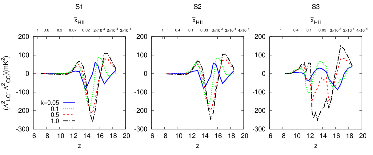
Finally, in Figure 7 we show the redshift evolution of the difference in the power spectra with and without the light-cone effect for the model C for the three source models at different scales. As expected, the difference is maximum at the peak and the trough regions found in the evolution of the power spectra. At large scales (), the difference can be as large as to . The difference is to at intermediate scales like . In principle, such a strong effect should easily be detected by future experiments like the SKA.
3.4 Effect of simulation box size
It has been found earlier by Datta et al. (2014) that the light-cone effect is larger when larger simulation box is used. In order to quantify the effect of box size on our results, we estimated the signal using a smaller box of length cMpc (in addition to our default box of cMpc). The results are shown in Fig. 8. In the left panel, we plot the evolution of at a scale Mpc-1 for the two boxes with and without the light-cone effect. As expected, the power spectra without the light-cone effect (thick lines) for the two boxes agree with each other. However, we can see that the light-cone effect is considerably less prominent for the smaller box in agreement with Datta et al. (2014). In particular, the smoothing of the three peak nature in the evolution plot of the power spectrum is more prominent for the larger box. The effect can be much more stronger in simulation box with size cMpc (Datta et al. 2014; Mesinger et al. 2014, e.g.,), which may completely smooth out the three peak nature of the evolution plot of the power spectrum. This will constrain us to choose smaller frequency bands during 21-cm experiments to avoid strong light-cone effects and restore the peakiness feature of the power spectrum which is very useful for parameter estimation etc. The same conclusions can be drawn from the right hand panel too where we have shown the ratio of the power spectra with and without the light-cone effect for Mpc-1. Clearly, the ratio deviates from unity quite prominently for the larger box compared to the smaller one.
3.5 Anisotropy from the light-cone effect
Since the light-cone effect modifies the 21-cm signal along the line of sight direction similar to the RSD, it is expected that it may cause anisotropies in the signal. This was investigated in detail by Datta et al. (2014) for a model similar to our model A, and they concluded that the light-cone effect does not induce any significant anisotropies in the signal. We confirm their findings for the model A. In addition, we find that the light-cone effect does not cause any prominent anisotropies for the models B and C too for relevant scales of interest. In fact, for large scales Mpc-1, our simulation box does not contain sufficient number of modes leading to large sample variance. Hence it is difficult to draw any significant conclusion on anisotropies at large scales.
In order to explain the effect in a somewhat simpler manner, we have calculated the ‘anisotropy ratio’ defined as (Fialkov et al. 2015, e.g.,):
| (6) |
where the averages are over angles. If the signal is isotropic then will be identically zero, otherwise it can be positive or negative. The redshift evolution of the anisotropy ratio for scales Mpc-1 is plotted in Figure 9. The source model chosen is . We find from the top panels that the RSD can cause significant anisotropies ( for Mpc-1) for all the three models1111 11 For the models B and C, the level of anisotropies arising from the RSD depends on the source model too. The anisotropies are caused by the correlation of the fluctuations with the dark matter density field, which is enhanced when small sources are included. For and which do not contain haloes smaller than , we find that from RSD effects (in agreement with results of Paper I).. The redshift where the is maximum corresponds to prominent dip in the evolution of the power spectrum.
In contrast, the light-cone effect does not cause any significant anisotropy on the signal as can be seen from the middle panels for the scales considered. The anisotropy, when both the effects are included, is thus dominated by the contribution from the RSD. We should mention here that it is possible that the anisotropy arising from light-cone effect behave differently for larger scales Mpc-1. In order to have sufficient number of modes at such large scales one requires boxes of much larger size which, unfortunately, are beyond the scope of this paper.
4 Summary and discussion
The main focus of the paper is to investigate the impact of the light-cone effect on the H i 21-cm signal from the cosmic dawn. The 21-cm brightness temperature maps are generated by post-processing a dark matter -body simulation with an 1-D radiative transfer code. In addition to the usual stellar-like sources, we have accounted for X-ray emitting mini-quasar like sources. The fluctuations in the spin temperature due to inhomogeneous coupling and heating of the IGM not only boost the 21-cm power spectrum but introduce several peaks and dips in it when plotted as a function of redshift. The boosted power spectrum, together with additional peaks and dips along the redshift axis, makes it an ideal case for studying the light-cone effect. Here, we calculate the spin temperature fluctuations self consistently for various possible source models and reionization histories. We then study, for the first time, the light-cone effect on the 21-cm power spectrum arising from the cosmic dawn when the signal is dominated by spin temperature fluctuations (unlike other previous studies which concentrated mainly on the ionization fluctuations).
The main findings of our work are summarised below:
- 1.
We find that our results are consistent with previous studies (Datta et al. 2014) for the model which assumes that the H i spin temperature to be fully coupled with the IGM temperature and very high compared to the CMB temperature throughout the reionization history (model A). The light-cone effect is most significant when the universe is and ionized as the spherical averaged power spectrum is increased/suppressed by a factor of and respectively. The effect is found to be minimum while the universe is ionized.
- 2.
The light-cone effect is much more dramatic in the model B where the inhomogeneous heating is taken into account. We find that the maximum suppression of the large-scale power spectrum due to the light-cone effect occurs around the two peaks and enhancement occurs around the dip between the two peaks when plotted against . We notice that the light-cone effect can increase the power spectrum by a factor of and times around redshift and respectively at large scales (). The suppression of the power spectrum around the peaks around redshifts and can be to at large scales. We find the enhancement/suppression to be higher for models where contributions of small sources have been included ( source model). Unlike the previous studies, we find a significant light-cone effect at small scales () as well at high redshifts.
In addition, when we calculate the coupling self-consistently (model C), we find that the power spectrum increases very rapidly at the very beginning of cosmic dawn and thus the light-cone effect can enhance the 21-cm power spectrum by a factor at large scales (). At these scales, the three peaks of the power spectrum are suppressed by factors of , and around redshifts and respectively. The light-cone effect can enhance the power spectrum in the dips by factors of and around redshift and respectively. In general, the light-cone effect at small scales is found to be smaller than the effect at larger scales, except during the cosmic dawn (may increase the power spectrum by factor of few at scales like ).
- 3.
Our results can be understood from the fact that the light-cone effect is strong in a situation where the power spectrum evolve non-linearly with redshift (or comoving distance) as any linear evolution gets cancelled out to a large extent (Datta et al. 2012a). Non-linear evolution of the 21-cm power spectrum is maximum when it takes a turn. For example, for the A model it happens twice, first time when and second time when . These are the places where the light-cone effect is very strong. For the B type model, one more peak in the power spectrum gets added. Because of this non-linear evolution around the heating peak, we see that the light-cone effect becomes very strong (power spectrum is suppressed substantially) around this peak. Similarly coupling inhomogeneities give rise to two more episodes of non-linear evolution of the power spectrum (one dip and one peak) in the very beginning of cosmic dawn where the light-cone effect is very strong.
- 4.
The large scale () power spectrum with light-cone effect included can differ by to mK2 from the case where light-cone effect is not included. The difference increases at small scales () to the range to mK2. In principle, such a strong effect should easily be detected by future experiments like the SKA. We also notice that the peaks and dips in the power spectrum are somewhat smoothed out due to the light-cone effect. It has been suggested (Mesinger et al. 2014, e.g.,) that the peaks can be used to extract source properties, X-ray and background etc. We argue that the light-cone effect should be considered while extracting those parameters from the peak and dip measurements.
- 5.
The light-cone effect can, in principle, introduce anisotropies in the power spectrum, similar to the RSD effects. It is somewhat difficult to predict the large scale Mpc-1 anisotropies because of the lack of number of modes in the simulation box. However, for intermediate scales Mpc-1, we do not find any significant anisotropy arising from the light-cone effect.
The light-cone effect, during the cosmic dawn ( is highly dependent on nature of the X-ray sources present during that time in the universe. For example, the heating of the IGM will be much more homogeneous if it is mainly driven by the HMXBs (Fialkov et al. 2014). In such a scenario the evolution of the signal will be solely dominated by the H i neutral fraction and thus the light-cone effect during the cosmic dawn will not be as strong as we see here. Although, we expect similar light-cone effect if supernova or hot inter-stellar gas dominate the X-ray budget since they are expected to have similar kind of SED like mini-quasars which emit large number of soft X-ray photons.
Finally, further investigation is required in order to understand the light-cone effect for different source models and reionization scenarios. The main result from this study is that the light-cone effect can change the amplitude of the 21-cm power spectrum as well as the shape of the evolution of the power spectrum at large scale quite substantially. Therefore, it is important that the effect is incorporated while modelling the 21-cm power spectrum, particularly during the cosmic dawn and early stages of reionization.
Acknowledgement
The simulations used in this work were performed on the IBM cluster hosted by the National Centre for Radio Astrophysics, Pune, India. KKD would like to thank DST for support through the project SR/FTP/PS-119/2012 and the University Grant Commission (UGC), India for support through UGC-faculty recharge scheme (UGC-FRP) vide ref. no. F.4-5(137-FRP)/2014(BSR).
References
- Alcock & Paczynski (1979) Alcock C., Paczynski B., 1979, Nature, 281, 358
- Ali, Bharadwaj & Pandey (2005) Ali S. S., Bharadwaj S., Pandey B., 2005, MNRAS, 363, 251
- Baek et al. (2009) Baek S., Di Matteo P., Semelin B., Combes F., Revaz Y., 2009, A&A, 495, 389
- Barkana & Loeb (2004) Barkana R., Loeb A., 2004, ApJ, 609, 474
- Barkana & Loeb (2005a) Barkana, R., & Loeb, A. 2005a, ApJ, 624, L65
- Barkana (2006) Barkana R., 2006, MNRAS, 372, 259
- Barkana & Loeb (2006) Barkana, R., & Loeb, A. 2006, MNRAS, 372, L43
- Becker et al. (2001) Becker, R. H., Fan, X., White, R. L., et al. 2001, AJ, 122, 2850
- Bharadwaj & Ali (2004) Bharadwaj, S., & Ali, S. S. 2004, MNRAS, 352, 142
- Bond et al. (1991) Bond J. R., Cole S., Efstathiou G., Kaiser N., 1991, ApJ, 379, 440
- Bowman et al. (2013) Bowman, J. D., Cairns, I., Kaplan, D. L., et al. 2013, Pub. Astro. Soc. Australia, 30, 31
- Choudhury & Ferrara (2006) Choudhury, T. R., & Ferrara, A. 2006, MNRAS, 371, L55
- Choudhury et al. (2009) Choudhury, T. R., Haehnelt, M. G., & Regan, J. 2009, MNRAS, 394, 960
- Datta et al. (2012a) Datta, K. K., Friedrich, M. M., Mellema, G., Iliev, I. T., & Shapiro, P. R. 2012a, MNRAS, 424, 762
- Datta et al. (2012b) Datta, K. K., Mellema, G., Mao, Y., et al. 2012b, MNRAS, 424, 1877
- Datta et al. (2014) Datta, K. K., Jensen, H., Majumdar, S., et al. 2014, MNRAS, 442, 1491
- Dayal et al. (2009a) Dayal P., Ferrara A., Saro A., Salvaterra R., Borgani S., Tornatore L., 2009, MNRAS, 400, 2000
- Dayal, Ferrara & Saro (2010) Dayal P., Ferrara A., Saro A., 2010, MNRAS, 402, 1449
- Elvis et al. (1994) Elvis M., et al., 1994, ApJS, 95, 1
- Fan et al. (2003) Fan, X., Strauss, M. A., Schneider, D. P., et al. 2003, AJ, 125, 1649
- Fan et al. (2006) Fan X., et al., 2006, AJ, 131, 1203
- Fialkov et al. (2014) Fialkov, A., Barkana, R., & Visbal, E. 2014, Nature, 506, 197
- Fialkov et al. (2015) Fialkov, A., Barkana, R., & Cohen, A. 2015, Physical Review Letters, 114, 101303
- Field (1958) Field G. B., 1958, Proc. I. R. E., 46, 240
- Fioc & Rocca (1997) Fioc M., Rocca V. B., 1997, A& A, 326, 950
- Fragos et al. (2013a) Fragos, T., Lehmer, B., Tremmel, M., et al. 2013, ApJ, 764, 41
- Fragos et al. (2013b) Fragos, T., Lehmer, B. D., Naoz, S., Zezas, A., & Basu-Zych, A. 2013, ApJ, 776, L31
- Furlanetto et al. (2004) Furlanetto, S. R., Zaldarriaga, M., & Hernquist, L. 2004, ApJ, 613, 1
- Furlanetto & Oh (2006) Furlanetto S. R., Oh S. P., 2006, ApJ, 652, 849
- Furlanetto et al. (2006) Furlanetto S. R., Oh S. P., Briggs F. H., 2006, Phys. Rep., 433, 181
- Ghara et al. (2015) Ghara, R., Choudhury, T. R., & Datta, K. K. 2015, MNRAS, 447, 1806
- Ghosh et al. (2012) Ghosh, A., Prasad, J., Bharadwaj, S., Ali, S. S., & Chengalur, J. N. 2012, MNRAS, 426, 3295
- Goto et al. (2011) Goto, T., Utsumi, Y., Hattori, T., Miyazaki, S., & Yamauchi, C. 2011, MNRAS, 415, L1
- Gunn & Peterson (1965) Gunn, J. E., & Peterson, B. A. 1965, ApJ, 142, 1633
- Harnois-Déraps et al. (2013) Harnois-Déraps, J., Pen, U.-L., Iliev, I. T., et al. 2013, MNRAS, 436, 540
- Iliev et al. (2006) Iliev I. T. et al., 2006, MNRAS, 371, 1057
- Jensen et al. (2013) Jensen, H., Datta, K. K., Mellema, G., et al. 2013, MNRAS, 435, 460
- Komatsu et al. (2011) Komatsu, E., Smith, K. M., Dunkley, J., et al. 2011, ApJS, 192, 18
- La Plante et al. (2014) La Plante, P., Battaglia, N., Natarajan, A., et al. 2014, ApJ, 789, 31
- Laor et al. (1997) Laor A., Fiore F., Elvis M., Wilkes B. J., McDowell J. C., 1997, ApJ, 477, 93
- Lewis et al. (2000) Lewis, A., Challinor, A., & Lasenby, A. 2000, ApJ, 538, 473
- Majumdar et al. (2013) Majumdar, S; Bharadwaj, S; Choudhury, T. Roy, 2013, MNRAS, 434, 1978
- Majumdar et al. (2014) Majumdar, S., Mellema, G., Datta, K. K., et al. 2014, MNRAS, 443, 2843
- Malhotra & Rhoads (2006) Malhotra, S., & Rhoads, J. E. 2006, ApJ, 647, L95
- Mao et al. (2012) Mao Y., et al., 2012, MNRAS, 422, 926–954
- McQuinn et al. (2007) McQuinn M., Lidz A., Zahn O., Dutta S., Hernquist L., Zaldarriaga M., 2007, MNRAS, 377, 1043
- Mellema et al. (2006) Mellema G., Iliev I. T., Pen U.-L., Shapiro P. R., 2006, MNRAS, 372, 679
- Mellema et al. (2013) Mellema, G., Koopmans, L. V. E., Abdalla, F. A., et al. 2013, Experimental Astronomy, 36, 235
- Mesinger & Furlanetto (2007) Mesinger, A., & Furlanetto, S. 2007, ApJ, 669, 663
- Mesinger et al. (2014) Mesinger, A., Ewall-Wice, A., & Hewitt, J. 2014, MNRAS, 439, 3262
- Mitra et al. (2011) Mitra, S., Choudhury, T. R., & Ferrara, A. 2011, MNRAS, 413, 1569
- Mitra et al. (2012) Mitra, S., Choudhury, T. R., & Ferrara, A. 2012, MNRAS, 419, 1480
- Morales & Wyithe (2010) Morales, M. F., & Wyithe, J. S. B. 2010, ARA&A, 48, 127
- Paciga et al. (2013) Paciga, G., Albert, J. G., Bandura, K., et al. 2013, MNRAS, 433, 639
- Geil & Wyithe (2008) Geil P. M., Wyithe J. S. B., 2008, MNRAS, 386, 1683
- Pacucci et al. (2014) Pacucci, F., Mesinger, A., Mineo, S., & Ferrara, A. 2014, MNRAS, 443, 678
- Paranjape & Choudhury (2014) Paranjape, A., & Choudhury, T. R. 2014, MNRAS, 442, 1470
- Parsons et al. (2014) Parsons, A. R., Liu, A., Aguirre, J. E., et al. 2014, ApJ, 788, 106
- Planck Collaboration et al. (2014) Planck Collaboration, Ade, P. A. R., Aghanim, N., et al. 2014, A&A, 571, A16
- Planck Collaboration et al. (2015) Planck Collaboration, Ade, P. A. R., Aghanim, N., et al. 2015, arXiv:1502.01589
- Pritchard & Loeb (2012) Pritchard, J. R., & Loeb, A. 2012, Reports on Progress in Physics, 75, 086901
- Robertson et al. (2015) Robertson, B. E., Ellis, R. S., Furlanetto, S. R., & Dunlop, J. S. 2015, ApJ, 802, L19
- Santos et al. (2008) Santos, M. G., Amblard, A., Pritchard, J., Trac, H., Cen, R., & Cooray, A. 2008, ApJ, 689, 1
- Shin, Trac & Cen (2008) Shin M.-S., Trac H., Cen R., 2008, ApJ, 681, 756
- Tingay et al. (2013) Tingay, S. J., Goeke, R., Bowman, J. D., et al. 2013, Pub. Astro. Soc. Australia, 30, 7
- Thomas et al. (2009) Thomas, R. M., et al. 2009, MNRAS, 393, 32
- Thomas & Zaroubi (2011) Thomas R. M., Zaroubi S., 2011, MNRAS, 410, 1377
- van Haarlem et al. (2013) van Haarlem, M. P., Wise, M. W., Gunst, A. W., et al. 2013, A&A, 556, A2
- Vanden Berk et al. (2001) Vanden Berk D. E., et al., 2001, AJ, 122, 549
- Vignali, Brandt, & Schneider (2003) Vignali C., Brandt W. N., Schneider D. P., 2003, AJ, 125, 433
- Wouthuysen (1952) Wouthuysen S. A., 1952, AJ, 57, 31
- Zahn et al. (2007) Zahn O., Lidz A., McQuinn M., Dutta S., Hernquist L., Zaldarriaga M., Furlanetto S. R., 2007, ApJ, 654, 12
- Zawada et al. (2014) Zawada, K., Semelin, B., Vonlanthen, P., Baek, S., & Revaz, Y. 2014, MNRAS, 439, 1615