跳到论文正文
W Papers独立论文阅读器 arXiv:1504.05474 论文正文 计算阅读时间 · 0%
引用这篇论文根据当前论文元数据生成,正式投稿前建议核对。


License: arXiv.org perpetual non-exclusive license
arXiv:1504.05474v2 [cs.IT] 13 Jul 2015

A Simple Algorithm for Approximation by Nomographic Functions

Steffen Limmer1, Jafar Mohammadi1 and Sławomir Stańczak12 Affiliation: 1 Fraunhofer Institute for Telecommunications, Heinrich Hertz Institute, Einsteinufer 37, 10587 Berlin, Germany.
2 Fachgebiet Informationstheorie und theoretische Informationstechnik,
Technische Universität Berlin, Einsteinufer 25, 10587 Berlin, Germany.
Abstract

This paper introduces a novel algorithmic solution for the approximation of a given multivariate function by a nomographic function that is composed of a one-dimensional continuous and monotone outer function and a sum of univariate continuous inner functions. We show that a suitable approximation can be obtained by solving a cone-constrained Rayleigh-Quotient optimization problem. The proposed approach is based on a combination of a dimensionwise function decomposition known as Analysis of Variance (ANOVA) and optimization over a class of monotone polynomials. An example is given to show that the proposed algorithm can be applied to solve problems in distributed function computation over multiple-access channels.

Index Terms: 
Distributed computation, nomographic approximation, compute-and-forward, multiple-access channel

I Introduction

Distributed function computation is not a new idea, however, there has been recently an emerging interest in communication strategies that use the wireless channel for function computation over multiple-access channels [1, 2]. Such strategies have the potential for huge performance gains expressed in terms of efficiency, complexity and signaling overhead. The approach of [2] exploits the superposition property of the wireless channel for computation of some nomographic functions and is of high practical relevance because it is robust under practical impairments such as the lack of synchronization; in addition, there is little need for coordination between different sensors. The recent work [8] demonstrates a hardware implementation of the method presented in [2]. A key ingredient thereby is that the function to be computed has a suitable nomographic representation that is used to match the process of function computation to the communication channel [1, 3]. However, in [1, 2, 3] an algorithmic method to obtain suitable nomographic representations of given functions is missing.

The theoretical analysis of functions that can be written in a nomographic form has a long history, which dates back to Kolmogorov [4], Sprecher [5, 6] and Buck [7]. The authors in [5] and [6] showed that every function has a nomographic representation, when the outer function can be discontinuous (e.g. a space-filling curve). Implementing such functions in digital signal processing systems, especially when based on space-filling curves as analysed in [6], is prohibitive and leads to designs that are notoriously susceptible to noise.

Since many known nomographic representations of functions used in wireless sensor network (WSN) applications are too intricate for practical use, we argue in favor of considering nomographic representations that approximate the functions of interest and are easy to implement in distributed networks.11 1 Notice that nomographic approximation is used in this paper to refer to a nomographic representation of some function that approximates the function of interest in some pre-defined sense. In this work, we propose a simple method for nomographic approximation that can be used to approximate functions dictated by given applications in a decentralized manner. In a nutshell, the proposed method can be used to approximate certain multivariate functions by means of some nomographic approximations that are composed of a monotone continuous outer function and continuous inner functions. When implemented in digital signal processing systems such inner and outer functions are more robust to noise and easier to compute with finite precision arithmetic. The proposed approach is an algorithmic way to approximate more functions to be computed via the methods in [1, 2].

I-A Notation

Scalars, vectors, matrices and sets are denoted by lowercase aa, bold lowercase 𝒂\bm{a}, bold uppercase 𝑨\bm{A} and calligraphic letters 𝒜\mathcal{A}, respectively. (⋅)T(\cdot)^{T}, f∘gf\circ g and f−1f^{-1} stand for transpose, function composition and function inverse. The sets of natural number, real numbers and D×DD\times D real symmetric matrices are denoted by ℕ\mathbb{N}, ℝ\mathbb{R} and 𝕊D×D\mathbb{S}^{D\times D}, while 𝟘\mathbb{0} is used to denote the vector of all zeros, where the size will be clear from the context. We use ℒp​(𝒳K)\mathcal{L}_{p}(\mathcal{X}^{K}) to refer to the space of pp-integrable (1≤p<∞1\leq p<\infty) real functions, 𝒫K,D​(𝒳K)\mathcal{P}_{K,D}(\mathcal{X}^{K}) to the space of square integrable real polynomials of KK variables of degree at most DD in each variable, 𝒞⁡(𝒳K)\mathcal{C}(\mathcal{X}^{K}) to the space of continuous functions, and 𝒩⁡(𝒳K)\mathcal{N}\left(\mathcal{X}^{K}\right) to the space of nomographic functions, i.e. functions that can be represented in the form ψ⁡(∑k=1Kφk​(xk))\psi(\sum_{k=1}^{K}\varphi_{k}(x_{k})), and all spaces defined on 𝒳K:=𝒳×…×𝒳⊆ℝK\mathcal{X}^{K}:=\mathcal{X}\times\ldots\times\mathcal{X}\subseteq\mathbb{R}^{K}, respectively. If in addition the outer and inner functions ψ\psi and φk\varphi_{k} fulfill φk∈𝒞⁡(𝒳):𝒳→Ωk⊆ℝ​∀k\varphi_{k}\in\mathcal{C}(\mathcal{X}):\mathcal{X}\to\Omega_{k}\subseteq\mathbb{R}\ \forall k and ψ∈𝒞⁡(Ω′):Ω′→Ω\psi\in\mathcal{C}(\Omega^{\prime}):\Omega^{\prime}\to\Omega, we denote the corresponding space by 𝒩𝒞​(𝒳K)\mathcal{N}_{\mathcal{C}}(\mathcal{X}^{K}) [3].

II System Model, Problem Statement and Theoretical Framework

We consider a network consisting of K∈ℕK\in\mathbb{N} sensors indexed by the set 𝒦:={1,…,K}\mathcal{K}:=\{1,\ldots,K\}. The sensors observe measurements 𝒙:=[𝒙1,…,𝒙𝑲]𝑻∈𝒳𝑲\bm{x}:=[x_{1},\ldots,x_{K}]^{T}\in\mathcal{X}^{K} and the task of the network is to compute or approximate a multivariate function

f:𝒳K→Ω⊆ℝ\displaystyle f:\mathcal{X}^{K}\to\Omega\subseteq\mathbb{R} (1)

at some pre-selected fusion node.22 2 Due to the structure of the nomographic representation, every ordinary sensor can act as fusion node. The underlying computation and communication scenario is illustrated in Fig. 1.

II-A Problem statement

It was shown in [2, 3] that a nomographic represenation of some given function admits an efficient reconstruction or estimation of this function over the wireless channel. Although every function has a nomographic representation of the form ψ⁡(∑k=1Kφk​(xk))\psi(\sum_{k=1}^{K}\varphi_{k}(x_{k})), the general construction of the inner functions and the outer function is not amenable to implementation on state-of-the-art hardware technologies. Therefore, given some function ff defined by (1), the problem is to find a suitable nomographic representation such that (in some sense)

f⁡(𝒙)≈ψ⁡(∑𝒌=1𝑲φ𝒌​(𝒙𝒌))∀𝒙∈𝒳𝑲.\displaystyle f(\bm{x})\approx\psi\Bigl(\sum\nolimits_{k=1}^{K}\varphi_{k}(x_{k})\Bigr)\quad\forall\bm{x}\in\mathcal{X}^{K}\,. (2)

In doing so, we assume the following:

  1. A.1

    ψ\psi is monotone continuous,

  2. A.2

    {φk}k∈𝒦\{\varphi_{k}\}_{k\in\mathcal{K}} are continuous,

which is based on practical considerations concerning noise robustness and implementability on digital signal processing systems.

Refer to caption
Refer to caption
Fig. 1: Separation and superposition based function compuation in networks.

To emphasize the importance of Assumptions A.1 and A.2 on the space of representable functions, let us review some previously known results from literature.

Fact 1.

Representation by nomographic functions

  1. 1.

    Let φk\varphi_{k} be monotone increasing, ψ\psi be possibly discontinuous, then we have [5, 6]

    f⁡(𝒙)=ψ⁡(∑𝒌=1𝑲φ𝒌​(𝒙𝒌)),∀𝒇∈𝒞⁡(𝒳𝑲).\displaystyle f(\bm{x})=\psi\Bigl(\sum\nolimits_{k=1}^{K}\varphi_{k}(x_{k})\Bigr)\,,\forall f\in\mathcal{C}(\mathcal{X}^{K})\,. (3)
  2. 2.

    Let φk∈𝒞⁡(ℝ)\varphi_{k}\in\mathcal{C}(\mathbb{R}), ψ∈𝒞⁡(ℝ)\psi\in\mathcal{C}(\mathbb{R}), then the following holds:

    • •

      𝒩𝒞​(𝒳K)\mathcal{N}_{\mathcal{C}}(\mathcal{X}^{K}) is a nowhere dense subset of 𝒞⁡(𝒳K)\mathcal{C}(\mathcal{X}^{K}) [7]

    • •

      f⁡(𝒙)=∑𝒊=12​𝑲+1ψ𝒊​(∑𝒌=1𝑲φ𝒌(𝒊)​(𝒙𝒌))f(\bm{x})=\sum\nolimits_{i=1}^{2K+1}\psi_{i}\Bigl(\sum_{k=1}^{K}\varphi_{k}^{(i)}(x_{k})\Bigr), i.e. every function can be written as a sum of at most 2​K+12K+1 nomographic functions [4].

Due to Assumptions A.1-2, we consider the second case and impose an additional constraint of a single function ψ\psi. Note that the implication of Fact 1.2) is that only a sparse subset of functions f∈𝒞⁡(𝒳K)f\in\mathcal{C}(\mathcal{X}^{K}) can be approximated by some f^∈𝒩𝒞​(𝒳K)\hat{f}\in\mathcal{N}_{\mathcal{C}}(\mathcal{X}^{K}) with arbitrary high precision. The derived framework provides a necessary condition for suitable f^\hat{f} to exist as well as the corresponding inner and outer functions.

II-B Theoretical framework: Analysis of variance

To establish our results, we resort to a general framework for a dimensionwise decomposition of a function f⁡(𝒙)f(\bm{x}) into a sum of lower-dimensional terms. More precisely, we consider the Analysis of Variance (ANOVA) framework [9, 10], which has also been considered in the context of many other applications, ranging from chemistry and finance to statistics (see e.g. [11]). The goal of this framework is to decompose a function f∈ℒ2​(𝒳K)f\in\mathcal{L}_{2}(\mathcal{X}^{K}) into a sum of 2K2^{K} functions f𝒮f_{\mathcal{S}} that are mutually orthogonal w.r.t. the inner product ⟨f,g⟩=∫𝒳Kf⁡(𝒙)⋅𝒈⁡(𝒙)​𝒅𝒙\langle f,g\rangle=\int_{\mathcal{X}^{K}}f(\bm{x})\cdot g(\bm{x})\ d\bm{x}. Here, the function ff is decomposed into a sum of lower dimensional functions

f⁡(𝒙)=∑𝒮⊆𝒦𝒇𝒮​(𝒙𝒮),\displaystyle f(\bm{x})=\sum\nolimits_{\mathcal{S}\subseteq\mathcal{K}}f_{\mathcal{S}}(\bm{x}_{\mathcal{S}}), (4)

where each function f𝒮f_{\mathcal{S}} only depends on a subset of variables indexed by the set 𝒮⊆𝒦\mathcal{S}\subseteq\mathcal{K} and the sum ranges over the power set of 𝒦\mathcal{K}. The algorithm to obtain the ANOVA decomposition for a given function f∈ℒ2​(𝒳K)f\in\mathcal{L}_{2}(\mathcal{X}^{K}) is given by Alg. 1.

Input: f∈ℒ2​(𝒳K)f\in\mathcal{L}_{2}(\mathcal{X}^{K})
Output: functions {f𝒮}𝒮⊆𝒦\{f_{\mathcal{S}}\}_{\mathcal{S}\subseteq\mathcal{K}}, variances σ2\sigma^{2}, {σ𝒮}𝒮⊆𝒦2\{\sigma_{\mathcal{S}}\}^{2}_{\mathcal{S}\subseteq\mathcal{K}}
f∅:=∫𝒳Kf⁡(𝒙)​𝒅𝒙f_{\emptyset}:=\int_{\mathcal{X}^{K}}f(\bm{x})\ d\bm{x}; σ∅:=0\sigma_{\emptyset}:=0;
for 𝒮⊆𝒦\mathcal{S}\subseteq\mathcal{K}, 𝒮≠∅\mathcal{S}\neq\emptyset) do  f𝒮​(𝒙𝒮):=∫𝒳𝑲−|𝒮|𝒇⁡(𝒙)​𝒅𝒙𝒦\𝒮−∑𝒰⊊𝒮𝒇𝒰​(𝒙𝒰)f_{\mathcal{S}}(\bm{x}_{\mathcal{S}}):=\int_{\mathcal{X}^{K-\lvert\mathcal{S}\rvert}}f(\bm{x})\ d\bm{x}_{\mathcal{K}\backslash\mathcal{S}}-\sum_{\mathcal{U}\subsetneq\mathcal{S}}f_{\mathcal{U}}(\bm{x}_{\mathcal{U}});
σ𝒮2:=∫𝒳|𝒮|f𝒮2​(𝒙𝒮)​𝒅𝒙𝒮\sigma_{\mathcal{S}}^{2}:=\int_{\mathcal{X}^{\lvert\mathcal{S}\rvert}}f_{\mathcal{S}}^{2}(\bm{x}_{\mathcal{S}})\ d\bm{x}_{\mathcal{S}};
end σ2:=∫𝒳Kf2​(𝒙)​𝒅𝒙−(∫𝒳𝑲𝒇⁡(𝒙)​𝒅𝒙)2≡∑𝒮⊆𝒦σ𝒮2\sigma^{2}:=\int_{\mathcal{X}^{K}}f^{2}(\bm{x})\ d\bm{x}-\left(\int_{\mathcal{X}^{K}}f(\bm{x})\ d\bm{x}\right)^{2}\equiv\sum_{\mathcal{S}\subseteq\mathcal{K}}\sigma_{\mathcal{S}}^{2};
Algorithm 1 ANOVA decomposition of ff [10].
Remark 1.

Despite its simple form, the reader should note that a numerical implementation of Alg. 1 is in general not trivial. In fact, the computation of all 2K2^{K} terms for a full decomposition becomes impracticable for moderate values of KK and the involved high-dimensional integrals need to exist and be well-defined. In addition to these requirements, the integrals might still be hard to obtain in analytical form and numerical approximation methods might be necessary. However, for some classes of functions including multivariate polynomials f∈𝒫K,D​(𝒳K)f\in\mathcal{P}_{K,D}(\mathcal{X}^{K}), we can easily obtain a truncated decomposition in closed form up to moderate values of KK.

The conditions for which a truncated decomposition provides a good approximation of the original function are made precise in the following definition.

Definition 1.

[10] A function f{f} is said to be of order dd if

f⁡(𝒙)=∑|𝒮|≤df𝒮​(𝒙𝒮)⇔∑|𝒮|≤𝒅σ𝒮2=σ2\displaystyle f({\bm{x}})=\sum\nolimits_{\lvert\mathcal{S}\rvert\leq d}f_{\mathcal{S}}(\bm{x}_{\mathcal{S}})\Leftrightarrow\sum\nolimits_{\lvert\mathcal{S}\rvert\leq d}\sigma_{\mathcal{S}}^{2}=\sigma^{2} (5)

and of effective superposition dimension dd if, for some given sufficiently small ε>0\varepsilon>0, there holds

∑|𝒮|≤dσ𝒮2≥(1−ε)​σ2,\sum\nolimits_{\lvert\mathcal{S}\rvert\leq d}\sigma_{\mathcal{S}}^{2}\geq(1-\varepsilon)\sigma^{2}, (6)

where f𝒮​(𝐱𝒮)f_{\mathcal{S}}(\bm{x}_{\mathcal{S}}), σ𝒮2\sigma_{\mathcal{S}}^{2} and σ2\sigma^{2} are obtained by Alg. 1.

In particular, if a function ff is of order one, there are no interactions between variables {xk}k∈𝒦\{x_{k}\}_{k\in\mathcal{K}} and there exists a parametrization of the form f⁡(𝒙)=∑|𝒮|≤1𝒇𝒮​(𝒙𝒮)≡∑𝒌=1𝑲𝒇𝒌​(𝒙𝒌)+𝒇∅f(\bm{x})=\sum\nolimits_{\lvert\mathcal{S}\rvert\leq 1}f_{\mathcal{S}}(x_{\mathcal{S}})\equiv\sum\nolimits_{k=1}^{K}f_{k}(x_{k})+f_{\emptyset} (resp. small interaction and approximate parametrization for effective superposition one33 3 For convenience, subsequent designations on the approximate case are only made when a precise distinction is necessary.). This parametrization is well-known in the literature as Generalized additive models [12, 13] and it forms the basis for the algorithm developed in the following.

III Outline of the proposed approach

To obtain a parametrization of type (2) the idea is to ”skew” the function ff with a bijection g∈𝒞:Ω→Ω′g\in\mathcal{C}:\Omega\to\Omega^{\prime}, such that the resulting function φ⁡(𝒙):=(𝒈∘𝒇)​(𝒙):𝒳→𝜴′\varphi(\bm{x}):=(g\circ f)(\bm{x}):\mathcal{X}\to\Omega^{\prime} is of order one according to Def. 1. Here, the required bijectiveness of gg ensures that a unique functional inverse ψ:=g−1∈𝒞\psi:=g^{-1}\in\mathcal{C} exists and the resulting parametrization in nomographic form can be given by

f⁡(𝒙)=(𝒈−1∘𝒈∘𝒇)​(𝒙)=ψ⁡(∑|𝒮|≤𝒅φ𝒮​(𝒙𝒮)).\displaystyle f(\bm{x})=(g^{-1}\circ g\circ f)(\bm{x})=\psi\Bigl(\sum\nolimits_{\lvert\mathcal{S}\rvert\leq d}\varphi_{\mathcal{S}}(x_{\mathcal{S}})\Bigr)\,. (7)

Accordingly, given some approximation constant ϵ>0\epsilon>0 in Def. 1, a nomographic approximation is obtained if φ⁡(𝒙)\varphi(\bm{x}) is of effective superposition dimension 11. These statements are summarized in the following Lemma.

Lemma 1.

Let f:𝒳K→Ω∈𝒞⁡(𝒳K)f:\mathcal{X}^{K}\to\Omega\in\mathcal{C}(\mathcal{X}^{K}) and g:Ω→Ω′∈𝒞⁡(Ω)g:\Omega\to\Omega^{\prime}\in\mathcal{C}(\Omega) be a bijection with inverse ψ:=g−1\psi:=g^{-1}. If φ⁡(𝐱):=(𝐠∘𝐟)​(𝐱)∈ℒ𝟐​(𝒳𝐊)\varphi(\bm{x}):=(g\circ f)(\bm{x})\in\mathcal{L}_{2}(\mathcal{X}^{K}) is of order 11, we obtain a nomographic representation f=ψ⁡(∑|𝒮|≤1φ𝒮​(x𝒮))f=\psi(\sum\nolimits_{\lvert\mathcal{S}\rvert\leq 1}\varphi_{\mathcal{S}}(x_{\mathcal{S}})) by the ANOVA decomposition of φ⁡(𝐱)\varphi(\bm{x}) and the identity (ψ∘g∘f)​(𝐱):=(ψ∘φ)​(𝐱)=ψ⁡(∑|𝒮|≤𝟏φ𝒮​(𝐱𝒮))(\psi\circ g\circ f)(\bm{x}):=(\psi\circ\varphi)(\bm{x})=\psi(\sum_{\lvert\mathcal{S}\rvert\leq 1}\varphi_{\mathcal{S}}(\bm{x}_{\mathcal{S}})). Similarly, if (g∘f)​(𝐱)(g\circ f)(\bm{x}) is of effective superposition dimension 11 (given ε>0\varepsilon>0), we obtain a nomographic approximation, where the approximation is optimal in an ℒ2\mathcal{L}_{2} sense (or, equivalently, the minimum variance sense) of the inner approximation problem [14].

Remark 2.

The reader should note however, that due to the usually nonlinear transformation by the outer function ψ\psi, this ℒ2\mathcal{L}_{2} optimality does not need to hold for the overall approximation error. Note also that bounding the resulting supremum norm of the approximation error sup𝐱∈𝒳𝐊|f−∑|𝒮|≤dφ𝒮​(x𝒮)|\sup_{\bm{x}\in\mathcal{X}^{K}}\lvert f-\sum\nolimits_{\lvert\mathcal{S}\rvert\leq d}\varphi_{\mathcal{S}}(x_{\mathcal{S}})\rvert is an interesting open problem but out of scope of this implementation-oriented paper. We highlight, that the required analysis seems to be quite challenging but might be similar in spirit to the simpler case of approximation with ridge functions (see e.g. [15]).

III-A A class of monotone polynomials

To obtain a computationally tractable set of continuous bijections gg, we consider a class of polynomials known as Bernstein polynomials:

Lemma 2.

[16] Let g⁡(ξ)∈𝒫1,D−1:=∑d=0D−1zd+1​ξdg(\xi)\in\mathcal{P}_{1,D-1}:=\sum_{d=0}^{D-1}{z}_{d+1}\xi^{d}, be a real polynomial of degree D−1D-1 defined on [0,1][0,1] with real coefficients 𝐳:=[z1,…,zD]{\bm{z}}:=[{z}_{1},\ldots,{z}_{D}] and 𝐌~∈ℝD×D\tilde{\bm{M}}\in\mathbb{R}^{D\times D} be a lower triangular matrix with entries given by [𝐌~]i,j=(i−1j−1)​(D−1j−1)−1​∀i≥j[\tilde{\bm{M}}]_{i,j}={i-1\choose j-1}{D-1\choose j-1}^{-1}\ \forall i\geq j, [𝐌~]i,j=0​∀i<j[\tilde{\bm{M}}]_{i,j}=0\ \forall i<j. Then it holds that

min𝑖​[𝑴~​𝒛]𝒊≤𝒈⁡(ξ)≤max𝒊​[𝑴~​𝒛]𝒊.\displaystyle\underset{i}{\min}\ [\tilde{\bm{M}}\bm{z}]_{i}\leq g(\xi)\leq\underset{i}{\max}\ [\tilde{\bm{M}}\bm{z}]_{i}. (8)

As a continuous function on a closed interval is bijective iff it is strictly monotone, we may obtain a suitable set of bijections by bounding g⁡(ξ)>0​∀ξ∈[0,1]g(\xi)>0\ \forall\ \xi\in[0,1] and integrating the polynomial g⁡(ξ)g(\xi) w.r.t. ξ\xi. A formal proposition characterizing the resulting set is given in the following:

Proposition 1.

Let g⁡(ξ)∈𝒫1,Dg(\xi)\in\mathcal{P}_{1,D} be a polynomial in ξ\xi of degree DD defined on [0,1][0,1]. Then, g⁡(ξ)g(\xi) is monotone and continuous on [0,1][0,1] if it holds that g∈𝒱⁡(𝐳,𝐜)⊂𝒫𝟏,𝐃g\in\mathcal{V}(\bm{z},c)\subset\mathcal{P}_{1,D} with

𝒱⁡(𝒛,𝒄):=\displaystyle\mathcal{V}(\bm{z},c):= {∑d=1Dzd​ξd+c|𝒛∈𝒵∖𝟘},\displaystyle\Bigl\{\sum\nolimits_{d=1}^{D}z_{d}\xi^{d}+c\ \Big|\ \bm{z}\in\mathcal{Z}\setminus\mathbb{0}\Bigr\}, (9)
𝒵\displaystyle\mathcal{Z} :={𝒛|𝑴𝒛≥0},\displaystyle:=\{\bm{z}|\bm{M}\bm{z}\geq 0\}, (10)
𝑴\displaystyle\bm{M} :=𝑴~​diag​([1,2,3,…,D]T).\displaystyle:=\tilde{\bm{M}}\mathrm{diag}\Bigl(\left[1,2,3,\ldots,D\right]^{T}\Bigr). (11)
Proof.

The proof follows from Lemma 2 by integration and comparison of terms. ∎

The reader should note, that 𝒵\mathcal{Z} defines a polyhedral cone (where the origin needs to be excluded to ensure strict monotonicity for the set 𝒱⁡(𝒛,𝒄)\mathcal{V}(\bm{z},c)) which makes it viable for practical optimization algorithms.

III-B Nomographic Approximation by cone-constrained Rayleigh quotient optimization

It remains to study the structure of the inner approximation problem. To this end, let g∈𝒫1,D⊃𝒱⁡(𝒛,𝒄)g\in\mathcal{P}_{1,D}\supset\mathcal{V}(\bm{z},c) with domain Ω:=[0,1]\Omega:=[0,1]. Then we can establish the following results on σ2\sigma^{2} and σk2\sigma_{k}^{2}.

Lemma 3.

Let g∈𝒫1,Dg\in\mathcal{P}_{1,D}, φ:=(g∘f)∈ℒ2​([0,1]K)\varphi:=(g\circ f)\in\mathcal{L}_{2}([0,1]^{K}) and f:[0,1]K→[0,1]f:[0,1]^{K}\to[0,1]. Then, it holds that σ2=∫[0,1]Kφ2​(𝐱)​𝐝𝐱−(∫[𝟎,𝟏]𝐊φ⁡(𝐱)​𝐝𝐱)𝟐\sigma^{2}=\int_{[0,1]^{K}}\varphi^{2}(\bm{x})\ d\bm{x}-\left(\int_{[0,1]^{K}}\varphi(\bm{x})\ d\bm{x}\right)^{2} can be written in quadratic form σ2=𝐳𝐓​𝐁𝐳\sigma^{2}=\bm{z}^{T}\bm{B}\bm{z} with 𝐁:=𝐁(𝟏)−𝐛(𝟐)​𝐛(𝟐),𝐓∈ℝ𝐃×𝐃\bm{B}:=\bm{B}^{(1)}-\bm{b}^{(2)}\bm{b}^{(2),T}\in\mathbb{R}^{D\times D} and

[𝑩(1)]𝒊𝒋:=∫[0,1]𝑲𝒇​(𝒙)𝒊+𝒋​𝒅𝒙,𝒃𝒊(2):=∫[0,1]𝑲𝒇​(𝒙)𝒊​𝒅𝒙\displaystyle[\bm{B}^{(1)}]_{ij}:=\int_{[0,1]^{K}}f(\bm{x})^{i+j}\ d\bm{x},\ {b}_{i}^{(2)}:=\int_{[0,1]^{K}}f(\bm{x})^{i}\ d\bm{x} (12)

which is independent of the chosen constant cc.

Proof.

The proof is deferred to Appendix A. ∎

Lemma 4.

Let gg, φ\varphi and ff be as in Lemma 3 and let the mixed integrals

[𝑨(1)​(𝒌)]i​j\displaystyle{[\bm{A}^{(1)}(k)}]_{ij} :=∫[0,1](∫[0,1]K−1f​(𝒙)𝒊​𝒅𝒙𝒦\𝒌CLOSE\displaystyle:=\int_{[0,1]}\bigg(\int_{[0,1]^{K-1}}f(\bm{x})^{i}\ d\bm{x}_{\mathcal{K}\backslash k} (13)
×∫[0,1]K−1f(𝒙)𝒋𝒅𝒙𝒦\𝒌)𝒅𝒙𝒌∀𝒌𝒊𝒏𝒦\displaystyle\times\int_{[0,1]^{K-1}}f(\bm{x})^{j}\ d\bm{x}_{\mathcal{K}\backslash k}\bigg)\ dx_{k}\ \forall kin\mathcal{K}

exist and be finite. Then, we have σk2=𝐳​𝐀𝐤𝐓​𝐳​∀𝐤∈𝒦\sigma_{k}^{2}=\bm{z}{{}^{T}}\bm{A}_{k}\bm{z}\ \forall k\in\mathcal{K} with

𝑨𝒌:=𝑨(1)​(𝒌)−𝒃(2)​𝒃(2),𝑻∈ℝ𝑫×𝑫.\displaystyle\bm{A}_{k}:=\bm{A}^{(1)}(k)-\bm{b}^{(2)}\bm{b}^{(2),T}\in\mathbb{R}^{D\times D}\,. (14)
Proof.

The proof is deferred to Appendix B. ∎

Now, with the above results in hand, we are in a position to state our main result.

Proposition 2.

Let gg, φ\varphi and ff be as in Lemma 3. Then, given some ε>0\varepsilon>0, a function f:[0,1]K→[0,1]f:[0,1]^{K}\to[0,1] has a nomographic approximation in accordance with Def. 1 and Rem. 2 with continuous and monotone outer function ψ\psi and continuous inner functions φk\varphi_{k} if and only if

(1−ε)≤max𝒛∈𝒵∖𝟘​𝒛𝑻​𝑨𝒛𝒛𝑻​𝑩𝒛,\displaystyle(1-\varepsilon)\leq\underset{\bm{z}\in\mathcal{Z}\setminus\mathbb{0}}{\max}\ \frac{\bm{z}^{T}{\bm{A}}\bm{z}}{\bm{z}^{T}{\bm{B}}\bm{z}}, (15)

where 𝐀=∑𝐤=𝟏𝐊𝐀𝐤\bm{A}=\sum_{k=1}^{K}\bm{A}_{k}, and the matrices 𝐀𝐤,𝐤=𝟏​…​𝐊\bm{A}_{k},k=1\dotsc K, 𝐁\bm{B} and 𝐌\bm{M} are given by Lemma 3, 4 and Prop. 1.

Proof.

Let ε∈(0,1)\varepsilon\in(0,1) be given and arbitrary. Then, by Def. 1 and (7), a function ff has a nomographic approximation if (and only if) there exists g∈𝒱⁡(𝒛)g\in\mathcal{V}(\bm{z}) such that φ​(𝒙)=(𝒈∘𝒇)​(𝒙)\varphi(\bm{x})=(g\circ f)(\bm{x}) is of effective superposition dimension 11 and (1−ε)≤R:=∑|𝒮|≤1σ𝒮2σ2=∑kσk2σ2(1-\varepsilon)\leq R:=\tfrac{\sum_{\lvert\mathcal{S}\rvert\leq 1}\sigma_{\mathcal{S}}^{2}}{\sigma^{2}}=\tfrac{\sum_{k}\sigma_{k}^{2}}{\sigma^{2}} where both σ𝒮2=σk2,k=1​…​K\sigma_{\mathcal{S}}^{2}=\sigma^{2}_{k},k=1\dotsc K, and σ2\sigma^{2} depend on 𝒛≠𝟘\bm{z}\neq\mathbb{0} (through the skewing function gg). Now taking the maximum (which exists) of R=R⁡(𝒛)R=R(\bm{z}) over all 𝒛∈𝒵∖𝟘\bm{z}\in\mathcal{Z}\setminus\mathbb{0}, and by considering Lemma 3 and Lemma 4 with (7), we can conclude that ff has a nomographic approximation if and only if (15) holds. ∎

By applying the matrix lift 𝒁:=𝒛𝒛𝑻\bm{Z}:=\bm{z}\bm{z}^{T}, one can show that if the matrix 𝑩\bm{B} is nonsingular, the optimization problem outlined in Prop. 2 can be recast as the generally nonconvex optimization problem

𝒁⋆∈argmax𝒁∈𝕊𝑫×𝑫\displaystyle\bm{Z}^{\star}\in\underset{\bm{Z}\in\mathbb{S}^{D\times D}}{\mathrm{argmax}}\ tr​{𝑨𝒁}\displaystyle\mathrm{tr}\left\{{\bm{A}}\bm{Z}\right\} (16a)
s.t.\displaystyle\mathrm{s.t.}\ tr​{𝑩𝒁}=δ\displaystyle\mathrm{tr}\left\{{\bm{B}}\bm{Z}\right\}=\delta (16b)
𝒁⪰𝟘\displaystyle\bm{Z}\succeq\mathbb{0} (16c)
[𝑴𝒁𝑴𝑻]𝒊,𝒋≥0​∀{𝒊,𝒋}∈𝒦2\displaystyle[\bm{M}\bm{Z}\bm{M}^{T}]_{i,j}\geq{0}\ \forall\ \{i,j\}\in\mathcal{K}^{2} (16d)
rank⁡(𝒁)=1.\displaystyle\mathrm{rank}(\bm{Z})=1. (16e)

Due to the high complexity of solving (16) directly, we apply a technique known as semidefinite relaxation [17] to the nonconvex semidefinite program by neglecting the (nonconvex) rank constraint (16e) first and solving the resulting convex SDP. Then, the candidate solution set for the original problem (16) is given by {±λ1​𝒒1}\{\pm\sqrt{\lambda_{1}}\bm{q}_{1}\}, where λ1\lambda_{1} and 𝒒1\bm{q}_{1} denote the largest eigenvalue and eigenvector of 𝒁⋆\bm{Z}^{\star}. The relaxation is tight, i.e. the solution 𝒛⋆∈𝒵∩{±λ1​𝒒1}\bm{z}^{\star}\in\mathcal{Z}\cap\{\pm\sqrt{\lambda_{1}}\bm{q}_{1}\} of the SDR coincides with the solution to (16) if rank⁡(𝒁⋆)=1\mathrm{rank}(\bm{Z}^{\star})=1. If the rank constraint is violated, the solution will in general be suboptimal. In this case, we apply a heuristic to obtain a suboptimal feasible solution

𝒛⋆∈𝒵∩{𝑴−1​(𝑴​λ1​𝒒1)+,𝑴−1​(−𝑴​λ1​𝒒1)+},\displaystyle\bm{z}^{\star}\in\mathcal{Z}\cap\Bigl\{\bm{M}^{-1}\left(\bm{M}\sqrt{\lambda_{1}}\bm{q}_{1}\right)_{+},\bm{M}^{-1}\left(-\bm{M}\sqrt{\lambda_{1}}\bm{q}_{1}\right)_{+}\Bigr\}, (17)

where (⋅)+(\cdot)_{+} denotes the projection onto the positive orthant. This heuristic is motivated by our simulation results, which show that applying the projection onto the positive orthant after transformation by the matrix 𝑴\bm{M} yields a numerically much more stable solution compared to applying the projection directly by computing

𝒛⋆∈argmin{𝒛|𝑴𝒛≥𝟘}​min⁡{∥𝒛−λ1​𝒒1∥22,∥𝒛+λ1​𝒒1∥22}.\displaystyle\bm{z}^{\star}\in\mathrm{argmin}_{\{\bm{z}|\bm{M}\bm{z}\geq\mathbb{0}\}}\min\bigl\{\lVert\bm{z}-\sqrt{\lambda_{1}}\bm{q}_{1}\rVert_{2}^{2},\lVert\bm{z}+\sqrt{\lambda_{1}}\bm{q}_{1}\rVert_{2}^{2}\bigr\}.

The resulting overall approximation algorithm is described in Alg. 2.44 4 In the spirit of reproducible research, the corresponding MATLAB implementation of Alg. 2 will be made available on one of the authors websites.

Input: f:[0,1]K→[0,1]f:[0,1]^{K}\to[0,1], DD
Output: {φ𝒮}|𝒮|≤1\{\varphi_{\mathcal{S}}\}_{\lvert\mathcal{S}\rvert\leq 1}, ψ\psi
(1) Compute 𝑨\bm{A}, 𝑩\bm{B}, 𝑴\bm{M} using Lemma 3, 4 and 2;
(2) Compute 𝒛⋆\bm{z}^{\star} by solving SDR of (16);
(3) Compute ANOVA for g⋆∘fg^{\star}\circ f with g⋆:=𝒱⁡(𝒛⋆)g^{\star}:=\mathcal{V}(\bm{z}^{\star});
(4) Compute ψ\psi using numerical inversion of g⋆g^{\star};
Algorithm 2 Approximation of ff by ψ⁡(∑|𝒮|≤1φ𝒮​(x𝒮))\psi(\sum\nolimits_{\lvert\mathcal{S}\rvert\leq 1}\varphi_{\mathcal{S}}(x_{\mathcal{S}})).

IV Numerical Results

To evaluate the performance of the proposed algorithm, we simulate a network with two sensors measuring x1x_{1} and x2x_{2} and one fusion node (see also Fig. 1) that are deployed to compute a desired function

f⁡(x1,x2)=19​(x1+x1​x2+x2)2\displaystyle f(x_{1},x_{2})=\frac{1}{9}\left(x_{1}+x_{1}x_{2}+x_{2}\right)^{2} (18)

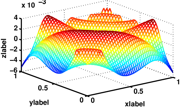
in a distributed manner. We choose the given example to highlight the impact of optimizing the skewing function to cancel out the interaction among the variables through the product x1​x2x_{1}x_{2}, where it is rather counter-intuitive that a good nomographic approximation exists. Many other interesting functions may come from data-driven models for distributed regression/classification using polynomial kernels which is beyond the scope of this paper. Using the algorithm described in Alg. 2 with skewing function gg of degree D=20D=20, we find a nomographic approximation with objective value ε=10−3\varepsilon=10^{-3}. The resulting functions and the overall approximation error are given in Table II and Fig. 2, where it can be seen in Fig. 2(f) that the resulting overall approximation error is bounded by |f−ψ⁡(∑|𝒮|≤1φ𝒮)|≤6×10⁻³\lvert f-\psi(\sum_{\lvert\mathcal{S}\rvert\leq 1}\varphi_{\mathcal{S}})\rvert\leq 6\times 10^{-3}. To highlight the effectiveness of using an optimized skewing function, the variances for approximation by a purely additive model (i.e. without using a skewing function) are given in Table I as a reference resulting in an objective value of ε=0.12\varepsilon=0.12.

σ{1}2=0.0168\sigma_{\{1\}}^{2}=0.0168 σ{2}2=0.0168\sigma_{\{2\}}^{2}=0.0168 σ{1,2}2=0.0043\sigma_{\{1,2\}}^{2}=0.0043
σ2=0.038\sigma^{2}=0.038 (σ{1}2+σ{2}2)​σ−2=0.88\Bigl(\sigma_{\{1\}}^{2}+\sigma_{\{2\}}^{2}\Bigr)\sigma^{-2}=0.88 ε=0.12\varepsilon=0.12
TABLE I: Direct evaluation of Alg. 1 for given test function.
z1,…,z5z_{1},\ldots,z_{5} z6,…,z10z_{6},\ldots,z_{10} z11,…,z15z_{11},\ldots,z_{15} z16,…,z20z_{16},\ldots,z_{20}
1.28031.2803 −134.14-134.14 442644.0442644.0 −366688.0-366688.0
−12.162-12.162 2637.02637.0 −697011.0-697011.0 145299.0145299.0
72.97572.975 −21534.0-21534.0 874766.0874766.0 −37288.0-37288.0
−236.66-236.66 84667.084667.0 −862822.0-862822.0 5220.65220.6
334.42334.42 −222633.0-222633.0 652977.0652977.0 −247.38-247.38
TABLE II: 𝒛⋆\bm{z}^{\star} obtained by Alg. 2 and D=20D=20.
Refer to caption
(a) Original function.
Refer to caption
(b) Value of the SDP (16) for varying degrees of the skewing function gg.
Refer to caption
(c) φ1​(x1)\varphi_{1}(x_{1}) obtained by Alg. 2 and D=20D=20.
Refer to caption
(d) φ2​(x2)\varphi_{2}(x_{2}) obtained by Alg. 2 and D=20D=20.
Refer to caption
(e) ψ\psi obtained by Alg. 2 and D=20D=20.
Refer to caption
(f) Approximation error e=f−ψ⁡(∑|𝒮|≤1φ𝒮)e=f-\psi(\sum_{\lvert\mathcal{S}\rvert\leq 1}\varphi_{\mathcal{S}}).
Fig. 2: Simulation results for Alg. 2 applied to the function f=19​(x1+x1​x2+x2)2f=\frac{1}{9}\left(x_{1}+x_{1}x_{2}+x_{2}\right)^{2}.

V Conclusion

In this paper, we studied the problem of nomographic approximation with continuous monotone outer function and continuous inner functions, which we expect to be of high practical relevance due to the amenability for distributed computation. By using a computationally tractable class of bijections based on Bernstein polynomials, we obtain a nomographic approximation with prescribed properties with respect to a defined distortion metric. The optimized approximation is obtained by the maximization of a cone-constrained Rayleigh-quotient. Since the problem is nonconvex, we consider its semidefinite relaxation. Though a precise characterization of the class of functions approximable in nomographic form with prescribed error metric still remains an open problem, we can see some interesting applications of the presented results, ranging from distributed learning and optimization to compressed classification.

References

  • [1] B. Nazer and M. Gastpar, “Computation over multiple-access channels,” IEEE Trans. Inf. Theory, vol. 53, no. 10, pp. 3498–3516, 2007.
  • [2] M. Goldenbaum and S. Stanczak, “Robust analog function computation via wireless multiple-access channels,” IEEE Trans. Comm., 2013.
  • [3] M. Goldenbaum, H. Boche, and S. Stanczak, “Harnessing interference for analog function computation in wireless sensor networks,” IEEE Trans. Signal Process., vol. 61, no. 20, pp. 4893–4906, 2013.
  • [4] A. N. Kolmogorov, “The representation of continuous functions of many variables by superposition of continuous functions of one variable and addition,” Proc. Amer. Math. Soc., 1957.
  • [5] D. A Sprecher, “A representation theorem for continuous functions of several variables,” Proc. Amer. Math. Soc., vol. 16, no. 2, pp. 200–203, 1965.
  • [6] D. A. Sprecher, “On computational algorithms for real-valued continuous functions of several variables,” Neural Netw., vol. 59, pp. 16–22, 2014.
  • [7] R. C. Buck, “Nomographic functions are nowhere dense,” Proc. Amer. Math. Soc., pp. 195–199, 1982.
  • [8] A. Kortke, M. Goldenbaum, and S. Stanczak, “Analog Computation Over the Wireless Channel: A Proof of Concept,” in Proc. IEEE Sensors, Valencia, Spain, Nov. 2014.
  • [9] E. Novak and H. Wozniakowski, Tractability of Multivariate Problems, vol. I: Linear Information, 2008.
  • [10] F. Kuo, I. Sloan, G. Wasilkowski, and H. Woźniakowski, “On decompositions of multivariate functions,” Math. Comp., vol. 79, no. 270, pp. 953–966, 2010.
  • [11] M. Griebel, Sparse grids and related approximation schemes for higher dimensional problems, 2005.
  • [12] T. J. Hastie and R. J. Tibshirani, Generalized additive models, vol. 43, CRC Press, 1990.
  • [13] F. Bach, “Breaking the curse of dimensionality with convex neural networks,” arXiv preprint arXiv:1412.8690, 2014.
  • [14] S. Rahman, “Approximation errors in truncated dimensional decompositions,” arXiv preprint arXiv:1310.6769, 2013.
  • [15] A. Kolleck and J. Vybiral, “On some aspects of approximation of ridge functions,” arXiv preprint arXiv:1406.1747, 2014.
  • [16] G. T. Cargo and O. Shisha, “The bernstein form of a polynomial,” J. Res. Nat. Bur. Stand. Sect. B, vol. 70, pp. 79, 1966.
  • [17] Z. Luo, W. Ma, A. M.-C. So, Y. Ye, and S. Zhang, “Semidefinite relaxation of quadratic optimization problems,” IEEE Signal Process. Mag., vol. 27, no. 3, pp. 20–34, 2010.

Appendix A Proof of σ2=𝒛𝑻​𝑩𝒛\sigma^{2}=\bm{z}^{T}\bm{B}\bm{z}, independence of cc

To show that σ2\sigma^{2} is independent of cc let g∈𝒫1,Dg\in\mathcal{P}_{1,D}, φ⁡(𝒙):=(𝒈∘𝒇)​(𝒙)∈ℒ2​(𝒳𝑲)\varphi(\bm{x}):=(g\circ f)(\bm{x})\in\mathcal{L}_{2}(\mathcal{X}^{K}), 𝒳K:=[0,1]K\mathcal{X}^{K}:=[0,1]^{K} and f:=f⁡(𝒙)f:=f(\bm{x}). Then

σ2\displaystyle\sigma^{2} =∫𝒳Kφ​(𝒙)2​𝒅𝒙⏟𝜟(1)−(∫𝒳𝑲φ⁡(𝒙)​𝒅𝒙)2⏟𝜟(2)\displaystyle=\underbrace{\int\nolimits_{\mathcal{X}^{K}}\varphi(\bm{x})^{2}\ d\bm{x}}_{\Delta^{(1)}}-\underbrace{\Bigl(\int_{\mathcal{X}^{K}}\varphi(\bm{x})\ d\bm{x}\Bigr)^{2}}_{\Delta^{(2)}}
Δ(1)\displaystyle\Delta^{(1)} =∫𝒳K(∑d=1Dzd​fd)2+2​c​∑d=1Dzd​fd+c2​𝑑𝒙\displaystyle=\int_{\mathcal{X}^{K}}\Bigl(\sum\nolimits_{d=1}^{D}z_{d}f^{d}\Bigr)^{2}+2c\sum\nolimits_{d=1}^{D}z_{d}f^{d}+c^{2}\ d\bm{x}
Δ(2)\displaystyle\Delta^{(2)} =(∫𝒳K∑d=1Dzd​fd​𝑑𝒙)2+∫𝒳𝑲2​𝒄​∑𝒅=1𝑫𝒛𝒅​𝒇𝒅+𝒄2​𝒅𝒙\displaystyle=\Bigl(\int_{\mathcal{X}^{K}}\sum\nolimits_{d=1}^{D}z_{d}f^{d}d\bm{x}\Bigr)^{2}+\int_{\mathcal{X}^{K}}2c\sum\nolimits_{d=1}^{D}z_{d}f^{d}+c^{2}\,d\bm{x}
σ2\displaystyle\sigma^{2} =∫𝒳K(∑d=1Dzd​fd)2​𝑑𝒙−(∑𝒅=1𝑫𝒛𝒅​∫𝒳𝑲𝒇𝒅​𝒅𝒙)2\displaystyle=\int_{\mathcal{X}^{K}}\Bigl(\sum_{d=1}^{D}z_{d}f^{d}\Bigr)^{2}\ d\bm{x}-\Bigl(\sum\nolimits_{d=1}^{D}z_{d}\int_{\mathcal{X}^{K}}f^{d}\ d\bm{x}\Bigr)^{2}

As 𝒛\bm{z} is independent of ff it follows by comparison of terms that σ2=𝒛𝑻​𝑩𝒛\sigma^{2}=\bm{z}^{T}\bm{B}\bm{z} with 𝑩:=𝑩(1)−𝒃(2)​𝒃(2),𝑻\bm{B}:=\bm{B}^{(1)}-\bm{b}^{(2)}\bm{b}^{(2),T} and

𝑩𝒊𝒋(1)\displaystyle\bm{B}_{ij}^{(1)} :=∫[0,1]Kfi+j​𝑑𝒙,{𝒊,𝒋}∈{1,…,𝑫}2\displaystyle:=\int_{[0,1]^{K}}f^{i+j}\ d\bm{x},\ \{i,j\}\in\{1,\ldots,D\}^{2}
𝒃𝒊(2)\displaystyle\bm{b}_{i}^{(2)} :=∫[0,1]Kfi​𝑑𝒙,𝒊∈{1,…,𝑫}.\displaystyle:=\int_{[0,1]^{K}}f^{i}\ d\bm{x},\ i\in\{1,\ldots,D\}.

Appendix B Proof of σk2=𝒛𝑻​𝑨𝒌​𝒛\sigma_{k}^{2}=\bm{z}^{T}\bm{A}_{k}\bm{z}, independence of cc

To show that σk2=𝒛𝑻​𝑨𝒌​𝒛\sigma_{k}^{2}=\bm{z}^{T}\bm{A}_{k}\bm{z} is independent of cc let gg, φ⁡(𝒙)\varphi(\bm{x}), 𝒳K\mathcal{X}^{K} and ff be as in Appendix A. Then

σk2\displaystyle\sigma_{k}^{2} =∫𝒳(∫𝒳K−1φ⁡(𝒙)​𝒅𝒙𝒦\𝒌−∫𝒳𝑲φ⁡(𝒙)​𝒅𝒙)2​d​xk\displaystyle=\int_{\mathcal{X}}\left(\int_{\mathcal{X}^{K-1}}\varphi(\bm{x})\ d\bm{x}_{\mathcal{K}\backslash k}-\int_{\mathcal{X}^{K}}\varphi(\bm{x})\ d\bm{x}\right)^{2}\ dx_{k}
=∫𝒳[∫𝒳K−1(∑d=1Dzd​fd+c)​d​𝒙𝒦\𝒌−∫𝒳𝑲(∑𝒅=1𝑫𝒛𝒅​𝒇𝒅+𝒄)​𝒅𝒙]2​d​xk\displaystyle=\int_{\mathcal{X}}\left[\int_{\mathcal{X}^{K-1}}\left(\sum_{d=1}^{D}z_{d}f^{d}+c\right)\ d\bm{x}_{\mathcal{K}\backslash k}-\int_{\mathcal{X}^{K}}\left(\sum_{d=1}^{D}z_{d}f^{d}+c\right)\ d\bm{x}\right]^{2}\ dx_{k}
=∫𝒳[∫𝒳K−1(∑d=1Dzd​fd+c)​d​𝒙𝒦\𝒌]2​d​xk+∫𝒳[∫𝒳K(∑d=1Dzd​fd+c)​𝑑𝒙]2​d​xk\displaystyle=\int_{\mathcal{X}}\left[\int_{\mathcal{X}^{K-1}}\left(\sum_{d=1}^{D}z_{d}f^{d}+c\right)\ d\bm{x}_{\mathcal{K}\backslash k}\right]^{2}\ dx_{k}+\int_{\mathcal{X}}\left[\int_{\mathcal{X}^{K}}\left(\sum_{d=1}^{D}z_{d}f^{d}+c\right)\ d\bm{x}\right]^{2}\ dx_{k}
−2∫𝒳[∫𝒳K−1(∑d=1Dzdfd+c)d𝒙𝒦\𝒌⋅∫𝒳𝑲(∑𝒅=1𝑫𝒇𝒅+𝒄)𝒅𝒙]dxk\displaystyle-2\int_{\mathcal{X}}\left[\int_{\mathcal{X}^{K-1}}\left(\sum_{d=1}^{D}z_{d}f^{d}+c\right)\ d\bm{x}_{\mathcal{K}\backslash k}\cdot\int_{\mathcal{X}^{K}}\left(\sum_{d=1}^{D}f^{d}+c\right)\ d\bm{x}\right]\ dx_{k}
=∫𝒳(∫𝒳K−1∑d=1Dfd​d​𝒙𝒦\𝒌)2​d​xk+2​c​∫𝒳[∫𝒳K−1∑d=1Dzd​fd​d​𝒙𝒦\𝒌]​d​xk+∫𝒳c2​d​xk\displaystyle=\int_{\mathcal{X}}\left(\int_{\mathcal{X}^{K-1}}\sum_{d=1}^{D}f^{d}\ d\bm{x}_{\mathcal{K}\backslash k}\right)^{2}\ dx_{k}+2c\int_{\mathcal{X}}\left[\int_{\mathcal{X}^{K-1}}\sum_{d=1}^{D}z_{d}f^{d}\ d\bm{x}_{\mathcal{K}\backslash k}\right]\ dx_{k}+\int_{\mathcal{X}}c^{2}\ dx_{k}
−2∫𝒳(∫𝒳K−1∑d=1Dzdfd)d𝒙𝒦\𝒌⋅∫𝒳𝑲∑𝒅=1𝑫𝒛𝒅𝒇𝒅𝒅𝒙)dxk\displaystyle-2\int_{\mathcal{X}}\left(\int_{\mathcal{X}^{K-1}}\sum_{d=1}^{D}z_{d}f^{d})\ d\bm{x}_{\mathcal{K}\backslash k}\cdot\int_{\mathcal{X}^{K}}\sum_{d=1}^{D}z_{d}f^{d}\ d\bm{x}\right)\ dx_{k}
−2c∫𝒳(∫𝒳K−1∑d=1Dzdfdd𝒙𝒦\𝒌)dxk−2c∫𝒳(∫𝒳K∑d=1Dzdfdd𝒙)dxk−2∫𝒳c2dxk\displaystyle-2c\int_{\mathcal{X}}\left(\int_{\mathcal{X}^{K-1}}\sum_{d=1}^{D}z_{d}f^{d}\ d\bm{x}_{\mathcal{K}\backslash k}\right)\ dx_{k}-2c\int_{\mathcal{X}}\left(\int_{\mathcal{X}^{K}}\sum_{d=1}^{D}z_{d}f^{d}\ d\bm{x}\right)\ dx_{k}-2\int_{\mathcal{X}}c^{2}\ dx_{k}
+∫𝒳(∫𝒳K∑d=1Dzdfdd𝒙)2dxk+2c∫𝒳(∫𝒳K∑d=1Dzdfdd𝒙)dxk+∫𝒳c2dxk,\displaystyle+\int_{\mathcal{X}}\left(\int_{\mathcal{X}^{K}}\sum_{d=1}^{D}z_{d}f^{d}\ d\bm{x}\right)^{2}\ dx_{k}+2c\int_{\mathcal{X}}\left(\int_{\mathcal{X}^{K}}\sum_{d=1}^{D}z_{d}f^{d}\ d\bm{x}\right)\ dx_{k}+\int_{\mathcal{X}}c^{2}\ dx_{k},

where we note that all terms involving cc vanish and we obtain

σk2\displaystyle\sigma_{k}^{2} =∫𝒳(∫𝒳K−1∑d=1Dzd​fd​d​𝒙𝒦\𝒌)2​d​xk⏟Γ(1)−2​∫𝒳(∫𝒳K−1∑d=1Dzd​fd​d​𝒙𝒦\𝒌⋅∫𝒳𝑲∑𝒅=1𝑫𝒛𝒅​𝒇𝒅​𝒅𝒙)​d​xk⏟Γ(2)\displaystyle=\underbrace{\int_{\mathcal{X}}\left(\int_{\mathcal{X}^{K-1}}\sum_{d=1}^{D}z_{d}f^{d}\ d\bm{x}_{\mathcal{K}\backslash k}\right)^{2}\ dx_{k}}_{\Gamma^{(1)}}-2\underbrace{\int_{\mathcal{X}}\left(\int_{\mathcal{X}^{K-1}}\sum_{d=1}^{D}z_{d}f^{d}\ d\bm{x}_{\mathcal{K}\backslash k}\cdot\int_{\mathcal{X}^{K}}\sum_{d=1}^{D}z_{d}f^{d}\ d\bm{x}\right)\ dx_{k}}_{\Gamma^{(2)}}
+∫𝒳(∫𝒳K∑d=1Dzd​fd​d𝒙)2​d​xk⏟Γ(3),with\displaystyle+\underbrace{\int_{\mathcal{X}}\left(\int_{\mathcal{X}^{K}}\sum_{d=1}^{D}z_{d}f^{d}\ d\bm{x}\right)^{2}\ dx_{k}}_{\Gamma^{(3)}},\mathrm{with}
Γ(1)\displaystyle\Gamma^{(1)} =∫𝒳(∫𝒳K−1∑d=1Dzd​fd​d​𝒙𝒦\𝒌)2​d​xk=∫𝒳(∑i=1D∑j=1Dzi​zj​∫𝒳K−1fi​d​𝒙𝒦\𝒌⋅∫𝒳𝑲−1𝒇𝒋​𝒅𝒙𝒦\𝒌)​d​xk\displaystyle=\int_{\mathcal{X}}\left(\int_{\mathcal{X}^{K-1}}\sum_{d=1}^{D}z_{d}f^{d}\ d\bm{x}_{\mathcal{K}\backslash k}\right)^{2}\ dx_{k}=\int_{\mathcal{X}}\left(\sum_{i=1}^{D}\sum_{j=1}^{D}z_{i}z_{j}\int_{\mathcal{X}^{K-1}}f^{i}\ d\bm{x}_{\mathcal{K}\backslash k}\cdot\int_{\mathcal{X}^{K-1}}f^{j}\ d\bm{x}_{\mathcal{K}\backslash k}\right)\ dx_{k}
=∑i=1D∑j=1Dzi​zj​∫𝒳(∫𝒳K−1fi​d​𝒙𝒦\𝒌⋅∫𝒳𝑲−1𝒇𝒋​𝒅𝒙𝒦\𝒌)​d​xk,\displaystyle=\sum_{i=1}^{D}\sum_{j=1}^{D}z_{i}z_{j}\int_{\mathcal{X}}\left(\int_{\mathcal{X}^{K-1}}f^{i}\ d\bm{x}_{\mathcal{K}\backslash k}\cdot\int_{\mathcal{X}^{K-1}}f^{j}\ d\bm{x}_{\mathcal{K}\backslash k}\right)\ dx_{k},

which can be written as Γ(1)=𝒛𝑻​𝑨(1)​(𝒌)​𝒛\Gamma^{(1)}=\bm{z}^{T}\bm{A}^{(1)}(k)\bm{z} with [𝑨(1)​(𝒌)]𝒊𝒋:=∫𝒳(∫𝒳𝑲−1𝒇𝒊​𝒅𝒙𝒦\𝒌⋅∫𝒳𝑲−1𝒇𝒋​𝒅𝒙𝒦\𝒌)​𝒅𝒙𝒌[\bm{A}^{(1)}(k)]_{ij}:=\int_{\mathcal{X}}\left(\int_{\mathcal{X}^{K-1}}f^{i}\ d\bm{x}_{\mathcal{K}\backslash k}\cdot\int_{\mathcal{X}^{K-1}}f^{j}\ d\bm{x}_{\mathcal{K}\backslash k}\right)\ dx_{k}. For the remaining terms we compute

Γ(2)\displaystyle\Gamma^{(2)} =∫𝒳(∫𝒳K−1∑d=1Dzd​fd​d​𝒙𝒦\𝒌⋅∫𝒳𝑲∑𝒅=1𝑫𝒛𝒅​𝒇𝒅​𝒅𝒙)​d​xk=∫𝒳(∫𝒳K−1∑d=1Dzd​fd​d​𝒙𝒦\𝒌⋅𝒃(2),𝑻​𝒛)​d​xk\displaystyle=\int_{\mathcal{X}}\left(\int_{\mathcal{X}^{K-1}}\sum_{d=1}^{D}z_{d}f^{d}\ d\bm{x}_{\mathcal{K}\backslash k}\cdot\int_{\mathcal{X}^{K}}\sum_{d=1}^{D}z_{d}f^{d}\ d\bm{x}\right)\ dx_{k}=\int_{\mathcal{X}}\left(\int_{\mathcal{X}^{K-1}}\sum_{d=1}^{D}z_{d}f^{d}\ d\bm{x}_{\mathcal{K}\backslash k}\cdot\bm{b}^{(2),T}\bm{z}\right)\ dx_{k}
=∫𝒳(∫𝒳K−1∑d=1Dzd​fd​d​𝒙𝒦\𝒌)​d​xk⋅𝒃(2),𝑻​𝒛=∫𝒳𝑲∑𝒅=1𝑫𝒛𝒅​𝒇𝒅​𝒅𝒙⋅𝒃(2),𝑻​𝒛=𝒛𝑻​𝒃(2)​𝒃(2),𝑻​𝒛\displaystyle=\int_{\mathcal{X}}\left(\int_{\mathcal{X}^{K-1}}\sum_{d=1}^{D}z_{d}f^{d}\ d\bm{x}_{\mathcal{K}\backslash k}\right)\ dx_{k}\cdot\bm{b}^{(2),T}\bm{z}=\int_{\mathcal{X}^{K}}\sum_{d=1}^{D}z_{d}f^{d}\ d\bm{x}\cdot\bm{b}^{(2),T}\bm{z}=\bm{z}^{T}\bm{b}^{(2)}\bm{b}^{(2),T}\bm{z}
Γ(3)\displaystyle\Gamma^{(3)} =∫𝒳(∫𝒳K∑d=1Dzdfdd𝒙)2dxk=∫𝒳[∑d=1Dzd∫𝒳Kfdd𝒙⋅∑𝒅=1𝑫𝒛𝒅∫𝒳𝑲𝒇𝒅𝒅𝒙)dxk=𝒛𝑻𝒃(2)𝒃(2),𝑻𝒛\displaystyle=\int_{\mathcal{X}}\left(\int_{\mathcal{X}^{K}}\sum_{d=1}^{D}z_{d}f^{d}\ d\bm{x}\right)^{2}\ dx_{k}=\int_{\mathcal{X}}\left[\sum_{d=1}^{D}z_{d}\int_{\mathcal{X}^{K}}f^{d}\ d\bm{x}\cdot\sum_{d=1}^{D}z_{d}\int_{\mathcal{X}^{K}}f^{d}\ d\bm{x}\right)\ dx_{k}=\bm{z}^{T}\bm{b}^{(2)}\bm{b}^{(2),T}\bm{z}

and obtain the desired result σk2=𝒛𝑻​[𝑨(1)​(𝒌)−2​𝒃(2)​𝒃(2),𝑻+𝒃(2)​𝒃(2),𝑻]​𝒛=𝒛𝑻​[𝑨(1)​(𝒌)−𝒃(2)​𝒃(2),𝑻]⏟𝑨𝒌​𝒛\sigma_{k}^{2}=\bm{z}^{T}\left[\bm{A}^{(1)}(k)-2\bm{b}^{(2)}\bm{b}^{(2),T}+\bm{b}^{(2)}\bm{b}^{(2),T}\right]\bm{z}=\bm{z}^{T}\underbrace{\left[\bm{A}^{(1)}(k)-\bm{b}^{(2)}\bm{b}^{(2),T}\right]}_{\bm{A}_{k}}\bm{z}.