Open systems dynamics: Simulating master equations in the computer
Abstract
Master equations are probably the most fundamental equations for anyone working in quantum optics in the presence of dissipation. In this context it is then incredibly useful to have efficient ways of coding and simulating such equations in the computer, and in this notes I try to introduce in a comprehensive way how do I do so, focusing on Matlab, but making it general enough so that it can be directly translated to any other language or software of choice. I inherited most of my methods from Juan José García-Ripoll (whose numerical abilities I cannot praise enough), changing them here and there to accommodate them to the way my (fairly limited) numerical brain works, and to connect them as much as possible to how I understand the theory behind them. At present, the notes focus on how to code master equations and find their steady state, but I hope soon I will be able to update them with time evolution methods, including how to deal with time-dependent master equations. During the last 4 years I’ve tested these methods in various different contexts, including circuit quantum electrodynamics, the laser problem, optical parametric oscillators, and optomechanical systems. Comments and (constructive) criticism are greatly welcome, and will be properly credited and acknowledged.
I On the structure of master equations and steady states
Let me start by briefly introducing in a greatly simplified manner the concepts of master equation and steady states. Consider a system endorsed with a Hilbert space of dimension (since we are interested in doing numerics, we will always assume that is finite, what might need truncating the Hilbert space dimension when this is infinite in reality). We say that the system is open when it is part of a larger space with which it exchanges energy, information, etc…, and generically we call environment to the rest of this larger space. In many situations, most notably when the environment is much larger or evolves much faster than the system, it is possible to describe the dynamics of the latter via a linear differential equation for its individual state, which of course is generally mixed since eliminating the environment means loosing information, hence requiring a description in terms of a density operator . We call master equation to the evolution equation for the system’s density operator, and in the following we will be guided by the generic form11 1 We will consider a single jump operator for notational simplicity, but everything we’ll do is generalized straightforwardly to the general irresversible term , or even to terms of different form.
| (1) |
where is an Hermitian operator containing the system Hamiltonian and coherent or reversible exchange processes with the environment, while is a so-called jump operator (with associated rate ) which describes irreversible processes such as excitations which are lost to the large environment never to come back to the system. is then an linear map usually called Liouvillian superoperator, whose name comes from the fact that it acts on operators to give operators.
Consider a basis , which allows us to represent the density operator as
| (2) |
with . The master equation, once projected into this basis, just provides a linear system of ordinary differential equations for the components of the density matrix, that is
| (3) |
with
In a more compact notation, it is customary to take the columns of the density matrix, and pile them one below the previous one, transforming the matrix into a vector
| (4) |
and the multidimensional array into a matrix , so that the previous equation is turned into the linear system
| (5) |
with solution
| (6) |
It is interesting to note the correspondence between the elements of the density matrix, and the elements of its vectorized form: . In the next section we will see that these expressions are much more than just a convenient way of reordering things.
From a practical point of view, if the Hilbert space dimension is not too large, then can be efficiently evaluated, and the main problem consists in how to write the matrix in an easy way, starting from the expression of the Liouvillian in the master equation (1). This is where superspace enters into play, and we will explain in the next section how it allows for a simple way of coding in the computer (Matlab in particular).
Let us now pass to discuss the important concept of steady state. For problems without selective measurements involved in the system+environment, the master equation must map states into states; this means that it is a trace preserving differential map, so that the condition is satisfied at all times, and hence the equations of (5) are not independent, but satisfy the constrain , the dot denoting time-derivative. This makes the rows (or columns) of the matrix linearly dependent, what ensures and hence that it exists at least one eigenvector with zero eigenvalue, which we will denote by , satisfying , where is a vector of zeros. The corresponding operator is called the steady state of the system, since in the absence of any other zero eigenvalue, this is the state towards which the system tends to as time evolves (the trace-preservation condition ensures also that all the other eigenvalues have negative real part, and hence for long times only survives).
One useful way of finding this steady state is as follows. First, given its defining equation , where is a vector of zeros, we replace one of the equations coming from the evolution equation of some some chosen diagonal element by the normalization condition , which can be additionally multiplied by any number , what is sometimes useful for numerical purposes; this means replacing the row number of by a vector of ’s in the elements multiplying the diagonal elements of , obtaining a new matrix , also replacing the vector by a vector containing a single non-zero entry at position . The steady state can then be found by solving the linear system , for example by inversion: . Later we will learn how to do this explicitly in Matlab.
II The master equation in superspace
The space where the density matrix is turned into a vector and the Liouvillian into a matrix is usually called superspace. Having operators as its elements, superspace can be defined formally as the tensor product of the Hilbert space and its dual, which indeed has vector space structure when endorsed with the trace product. As we will see in the next section, this gives us a simple way of representing superoperators by using simple tools of computer programs such as the Kronecker product, which is a built-in operation in both in Matlab and Mathematica. Instead of recalling the dual space, it is computationally more convenient to define superspace in a slightly simpler way: given an operator with matrix elements , we just associate to every index a fictitious -dimensional Hilbert space with basis , in which we describe the operator as a vector
| (7) |
We will say that is the abstract superspace representation of the operator . Note that its representation in the basis of superspace is the vector obtained by piling up the columns of the matrix formed by the elements one below the previous one, but only provided that the order of the superspace basis is chosen as22 2 Convince yourself of this fact through some simple examples. For example, the first element of the second column, , should correspond to the element in the superspace vector, , and this is precisely what the map provides. .
Consider now two operators and , and a superoperator acting on an operator as , expression which reads in superspace as
| (8) |
Taking into account that and are operators defined in the original -dimensional Hilbert space , so that they act on basis elements of the new fictitious spaces in the usual way (e.g., ), we can alternatively write
| (9) |
showing that in superspace the action of operators on the left (right), corresponds to actions of the (transpose) operator on the first (second) fictitious Hilbert space.
Hence, in superspace the master equation can be written as
| (10) |
where is the identity operator.
III Implementing the superspace ideas in Matlab
Let’s pass now to discuss how to implement the previous ideas in one particular program, Matlab, although similar tricks can be used in Mathematica, for example.
First, let us remind the notation, since I wouldn’t be surprised if everyone is lost on it at this point; to complicate things a bit, we will even need to introduce some more. The (column) vector representation of the basis elements of the Hilbert spaces or will be denoted by , with self-representation elements . Similarly, the superspace basis will have a vector representation , with self representation . Given an operator , its matrix elements are denoted by , and the matrix that they form by , which is nothing but the matrix representation of the operator in the chosen basis. The ‘vectorized’ form of this matrix, that is, the vector formed by piling up the columns of the matrix one below the next, is denoted by , and, as explained above, it can be seen as the representation of the operator in superspace, which we will still denote as , provided that the basis elements of superspace are ordered in the proper way. Hence, summing up, is the abstract notation for the operator acting on the original space and the one for the operator defined in superspace , with corresponding matrix and vector representations and , respectively. As for superoperators, take the Liouvillian as an example, we will refer to them as in calligraphic font33 3 Not to confuse with the notation for Hilbert spaces, for which we also use calligraphic font, but it should be clear from the context when we mean one or the other. when talking about them in an abstract way, and in blackboard font when referring to their matrix representation in superspace. For example, the right hand side of master equation (1) reads in an abstract way, and as once represented in superspace.
Let’s start from the basics of coding things in Matlab. The matrix representation of an operator can be written in Matlab (known their matrix elements ) as
| (11) |
where the commas can be replaced by a space. If we want to work with sparse matrices to save memory (useful for Hilbert spaces with large dimension, e.g., ), we can do so by replacing the matrix by44 4 From now on, Matlab functions will be highlighted by using typewriter font. sparse(); once in sparse form, we can always come back to the non-sparse one as full().
Let’s talk about basic matrix operations. Element is accessed as , while the whole column can be accessed as , and similarly for row , . We can access its -th diagonal as which generates a column vector with the desired diagonal. Given another matrix , is the matrix sum or difference, * is the matrix multiplication, * is the element-by-element multiplication, is the matrix multiplication of and , and is the matrix multiplication of and , where the inverse of can also be obtained as inv (but it is not recommended by Matlab, since it is slower than or ). We can find the determinant and trace as det and trace. The Hermitian conjugate of is obtained in Matlab as , while generates the transpose of . The exponential matrix is obtained as expm, while exp just exponentiates the elements of the matrix individually. As for the eigensystem, generates a vector with the eigenvalues of , while if we write eig, the eigenvectors are codified as columns of and is a diagonal matrix containing the corresponding eigenvalues. This operation cannot be used when is sparse, in which case we need to use eigs, which by default gives the 6 eigenvalues with largest magnitude; if we want a different number of eigenvalues, say , we can write eigs‘’, where L (S) means that we want the eigenvalues with the largest (smallest) magnitude if M, or real part if R. It is very useful to type help F in Matlab’s command window to get more info about some function F (for example, try help eig to find what else can be done with eig).
The vectorized form of the operator is obtained as . This is one of the reasons why we chose to pile columns instead of rows when vectorizing matrix representations of operators: in Matlab this operation is written with a single order, while in the case of rows, we would need to first transpose the matrix, and then give the order. On the other hand, given the matrix in vectorized form, we can always bring it back to matrix form as reshape.
The matrix representation of the identity operator can be written as eye, or speye when working with sparse matrices. The basis vector can be defined as . Similarly, defining the identity matrix in dimensions eye, the basis vector in superspace is obtained as .
Let’s move on to the tensor product operation. It is customary in quantum mechanics to represent the tensor product of two operators or vectors as the Kronecker product of their representations. In particular, given the matrix representations and of two operators and , their Kronecker product is defined as
| (12) |
and this is usually the representation chosen for the tensor product operator . However, it is important to understand that this is just one possible representation of the tensor product, corresponding to one particular ordering of the tensor product basis in the composite Hilbert space (superspace in our case). More concretly, note that according to the previous definition, given the vector representation of the basis element (or ), the Kronecker product representation of the basis element (or ) generates a vector with a single nonzero entry at position , that is, the superspace basis vector55 5 Convince yourself of this fact by working out some examples, e.g., in dimension 3 (), the Kronecker product of and , generates the vector , while the Kronecker product of and generates . These examples coincide precisely with the mapping . . However, as explained in the previous section, we would like to associate instead the superspace basis vector to the tensor product basis element , what means that we will not be using the usual Kronecker product representation of the tensor product, but one in reversed order: given the matrix representations and of two operators and , the representation of their tensor product is taken as their Kronecker product in reversed order, that is,
| (13) |
With this choice, the representation of the basis element corresponds to as we wanted to.
The Kronecker product is already implemented in Matlab through the operation kron (and same in Mathematica), which preserves the sparse character of the matrices. Hence, we can generate the vector representation of , by applying the kron operation in the reversed order kron.
Consider now two operators and , and a superoperator which acts on a third operator as . As explained in the previous section, in superspace this is rewritten as in an abstract way, expression which can be represented in the basis of superspace as kron* in Matlab code. Hence, the matrix representation of in superspace is written in Matlab as kron.
Let me remark that the choice of using the reversed kron order for the representation of the tensor product has been made for convenience in Matlab (to create the vectorized form of any operator with a single instruction, and for more things that will appear in the next section when dealing with composite Hilbert spaces). However, in other languages such as Mathematica, it can be better to stick to the traditional Kronecker product representation of the tensor product. But above all, what is important to understand what one is doing, and hence I strongly encourage the reader to think deeply about this, and play with some examples to interiorize this tricky point.
Hence, as promised, the matrix representation of the Liouvillian superoperator admits a very simple coding in Matlab:
| (14) |
where 1i is the proper way of writing the imaginary unit in Matlab, while conjz is how the complex conjugate of z looks in Matlab.
Once we have the Liouvillian superoperator, the next issue concerns finding the steady state of the system. If the Hilbert space dimension is not too large, we can try diagonalizing fully using eig. To access the steady state we can just find the index of the zero eigenvalue and get the corresponding column of , or proceed in a more elegant and automatic way, by sorting the order in which the eigenvalues appear. In particular, given the vector of eigenvalues diag, we generate a vector containing the indices of the permutation which we need to apply to reorder the eigenvectors in decreasing real part as sortreal‘descend’, where we additionally get the vector of sorted real parts , which we won’t use; once we have , we can sort the eigensystem as and , and the first column of the sorted should correspond now to the steady state , most likely requiring the additional normalization tracereshape to ensure it has unit trace. Now, for larger size problems, we will need to use sparse matrices, in which case the simplest way of finding the steady state would be as eigs‘LR’, which might require additional normalization as in the previous line. The density matrix of the steady state can then be found as reshape.
Even though in most cases the previous way of finding is enough, it is interesting to know how to implement the method which we introduced at the end of the first section, which consisted in replacing one equation of by the normalization condition , where is a parameter which we can choose as we wish. This is easily done in Matlab as follows (there are indeed many different ways of doing this, here I just pick the one I find simplest and most direct to code). First, we pick the index of the diagonal element whose equation we want to replace, with corresponding superindex . Then, we just define the matrix , and replace the corresponding row as *, which simply puts on the entries multiplying the diagonal elements of the density matrix. Then we define the vector with a single on element , which indeed corresponds to the superspace basis element multiplied by , that is, we can simply code it as *. Once we have done this, can be found as inv*, or by asking Matlab to solve the linear system as linsolve, which uses LU factorization. Note that we need to check that det, as otherwise we will have degenerate steady states, and the method will fail.
IV Dealing with composite Hilbert spaces
Everything we introduced up to now is general, in the sense that it applies to a system with any Hilbert space . Here I want to discuss some special features that appear when the system is a composition of simpler subsystems (two- or three-level systems, harmonic oscillators, etc…), in which case the Hilbert space has the tensor product structure . This is the scenario that we usually find in quantum optics, where typical systems are composed of atoms (maybe artificial such as superconducting qubits or quantum dots), and/or photonic, phononic, or motional modes.
Given a basis of subspace with dimension , a basis of the full Hilbert space can be built as , where is the dimension of the complete Hilbert space. Hence, each value of the index which we were using in the previous sections corresponds now to some multi-index labeling the basis elements of the Hilbert space of each subsystem. The point is that in many cases (for example when wanting to evaluate partial traces or transpositions) it is important to keep track of all the indices, and here I want to discuss how to deal with these issues by using efficient computational tools.
We have already encountered tensor products before when building the superspace, and we saw how to code them efficiently using the Kronecker product; we will again use the kron operation to deal with composite Hilbert spaces, but with a few subtle points. Let us start with the simplest structure in the composite Hilbert space: let’s represent its basis. Consider again the basis of subspace , and define the identity matrix of the corresponding dimension, eye, from which we build the vector representation of as . Then, we will represent a basis element of the complete Hilbert space corresponding to some multi-index , that is, , as the vector kronkronkron, where we use again a reversed order in the kron operations for future convenience, see the next paragraph. Taking into account that we still want to define as a vector with zeros and a one at position , which is the natural self-representation of the basis elements in the complete Hilbert space, the previous definition fixes the relation between and the multi-index to
| (15) |
Consider now a pure state in the complete Hilbert space. As explained, it would be useful to be able to move between this expression, and the one making explicit reference to the indices of each subspace, that is, . This is very easy to do in Matlab once we have made all the previous definitions. In particular, given the (column) vector representation of the state or better in Matlab code, we can transform it into a multidimensional array as reshape, from which is simply accessed as ; in the following we will use the double dot on top of the bold-faced symbol to denote that it is a multidimensional array. The multidimensional array can be transformed back to its vector form in the full Hilbert space just vectorizing it as . Note that the dimensions used to reshape the vector and the indices of the multidimensional array, follow the intuitive order that one would assign; this is thanks to using the reversed order in the kron operation, and would not be the case if we would have chosen the intuitive one.
At this point it should be clear that, given substates with vector representation or in Matlab code, the vector representation of the tensor product state can be obtained in Matlab as kronkronkron, with elements , given by (15).
We see then that dealing with vectors is not so difficult. Now let’s consider operators, which are a bit more tricky. Let’s start with a simple generalization of what we did for vectors. Consider an operator in the complete Hilbert space. Given its matrix representation in Matlab (with elements ) we would like to be able to retrieve the multi-index elements defined from
| (16) |
Similarly to vectors, this can be done by redefining as a multi-dimensional array reshape, from which we can then get the desired multi-index elements as . We can always go back to the original matrix representation in the complete Hilbert space by reshaping the multidimensional array as reshape.
Sometimes it is useful to have access to a different set of multi-index elements defined by
| (17) |
For this, the best is first building the multidimensional array as we explained above, and then use the extremely useful permute operation, which allows to permute indices of multidimensional arrays. In particular, defining another multidimensional array permute, we then access the desired multi-index elements as . In the following we will use the notation for the multidimensional array corresponding to the order of the multi-index elements, and the notation for the one corresponding to the order.
Imagine now that we are given a set of operators acting on the subspaces , with corresponding matrix representations . Our goal now is finding the different representations of the operator acting on the complete Hilbert space. Our starting point will be the Kronecker product kronkronkron; even though this is a matrix containing the elements of the representation of in the complete basis , it is easy to see that these elements are not ordered in the right way, and hence, in order for to coincide with the proper matrix representation of we need to reorder its elements. To this aim, we first build the multidimensional array reshape which has as its elements. Then, we can reorder its indices as permute, creating a multidimensional array which has as its elements. Finally, we find the matrix representation of in the complete Hilbert space as reshape. Hence, essentially we have followed the path of the previous paragraphs, but in reverse order. I hope all the manipulations have served to gain intuition about the operations kron, reshape, and permute, which allow for efficient and clean ways of representing Hilbert space objects in the computer.
Finally, I would like to discuss two operations very relevant in the context of composite Hilbert spaces: the partial transposition and the partial trace of an operator. Consider an operator acting on the complete Hilbert space. We define the operator corresponding to a partial transpose of with respect to subspace as
| (18) |
The different multidimensional array representations of this operator are easily obtained in Matlab from the ones of the original operator as permute or permute, and its matrix representation in the complete Hilbert space is then obtained as reshape. This is intuitively generalized to the case in which we want to perform partial transposition with respect to several subspaces; for example, if we want to transpose subspaces and (), then
| (19a) | ||||
| (19b) | ||||
| (19c) | ||||
As for the partial trace over subspace , denoted by or , it is defined as the operator
| (20) | ||||
that is, as the operators with elements corresponding to the contraction of the indices associated to the subspace. We can find again the different representations of this operator efficiently using Matlab’s built-in functions. In particular, we can find the multidimensional array corresponding to this operator as follows (we proceed by sequentially updating its definition): first, we bring the indices that we want to contract to the end of the array, permute; defining the dimension of the total Hilbert space after tracing out the desired subspace by , we reshape the previous array as a dimensional matrix, reshape; given the identity matrix of dimension denoted by eye, in terms of the previous matrix the contraction we are looking for is just *; the previous operation leaves us with a column vector with components, which we can finally reshape to give the multidimensional array we are looking for, reshape; finally, we find the matrix representation of the operator in the (remaining) complete Hilbert space as reshape. Of course, a similar trick can be done starting from the other multidimensional array ; also, the method is straightforwardly generalized to when we want to trace out several subspaces at once (maybe it’s a good thing to try these two things out as an exercise, to really discover if you understood all these constructions properly).
Let me finally remark once more that the only reason why we have choosen the reversed order in the kron operation is to make the coding simpler in Matlab. In particular, by just sticking to the simple rule “every time a tensor product appears, it is coded as the kron product in the reversed order”, the rest of manipulations are compactly and intuitively coded in Matlab as shown above, what would not be the case otherwise.
V An example: three-level cascade system interacting with two quantized optical modes
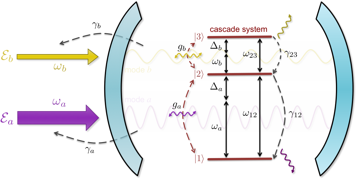
In order to fix ideas, let’s consider one example consisting in a three-level cascade system interacting with two driven modes of a cavity which we call and , see Fig. 1. Let us first discuss the structure of this system’s Hilbert space as well as a convenient way of writing the master equation governing its evolution, and then we will show how to code what we need in Matlab.
V.1 Hilbert space structure and master equation
The complete Hilbert space of this system can be written as . is the subspace of the system, with basis , which allows us to define the operators . and are the subspaces of the cavity modes, both spanned by Fock states , from which we define the basic annihilation operator for mode , and similarly for mode , whose corresponding annihilation operator we denote by . Note that and are Hilbert spaces of infinite dimension, but the computer can only deal with finite dimension; hence, we need to truncate the Fock state bases to a certain maximum photon number, which we will denote by and for the corresponding modes, leading to finite-dimensional bases and which approximately span and , respectively.
As shown in the figure, we order the states of the system such that corresponds to the excited state, to the middle one, and to the ground one, taking the energy origin in the middle state; we name and the frequencies of the corresponding transitions. Mode connects the transition and has resonance frequency , detuned by from the transition of the system. Mode connects the transition and has resonance frequency . We assume that both modes are driven by resonant lasers and decay through the partially reflecting mirror at rates and (the other mirror is assumed to have perfect reflectivity, although that’s not important for this simple example). Levels and of the system might decay through modes different than the cavity ones, what causes them spontaneous emission to levels and , respectively, at rates and . All these processes are captured by the following master equation in the Schrödinger picture:
| (21) |
where , with
| (22a) | ||||
| (22b) | ||||
| (22c) | ||||
| and where we have introduced the notation , given an operator . Note that we are not writing tensor products explicitly, and hence objects like must be understood as ; we will stick to this economic notation except when it can lead to a misunderstanding or we want to show the underlaying tensor product structure of the Hilbert space explicitly for some reason. | ||||
Unfortunately, there are two properties of this master equation that make it very difficult to deal with numerically. First, it is explicitly time-dependent through . Second, for large driving amplitudes it is to be expected that the cavity modes will get highly populated, and we will not be able to truncate the Fock bases to small enough and . Both these problems appear typically in many systems, and up to a point can be solved by moving to a different picture66 6 Recall that given the master equation (1), where the Hamiltonian can even be time-dependent, and a general time-dependent unitary , it is simple to prove that the transformed state evolves according to the master equation (22d) with new Hamiltonian and jump operators ., as we will learn now. The idea consists in doing two changes of picture (it can be done at once, but it’s more clear in two steps). First, we move to a picture rotating at the laser frequencies (which in this example coincide with the cavity frequencies); this is defined by the unitary transformation with , so that the transformed state evolves according to77 7 Note that we use here , and (22e) easy to prove from the Baker-Campbell-Haussdorf lemma (22f) and the commutators and .
| (23) |
with , where
| (24) |
Hence, we see that in this picture the master equation becomes time-independent. From this new picture we move to another one in which, in loose terms, the photons generated by the coherent drivings are already taken into account, so that we don’t need to ‘count’ them in the simulation. More specifically, this picture is defined by the unitary (displacement) transformation , which depends on two time-dependent amplitudes and that will be chosen later. In this case, the transformed state evolves according to88 8 This can be proved by using (25) together with (26)
| (27) | ||||
where , with
| (28) |
This master equation suggests choosing and such that its last term is cancelled, that is, as solutions of and :
| (29) |
Note that with this change of picture we have introduced time dependence in the master equation; however, since we are only interested in the long-time behavior of the system (steady state), and moreover, we can choose and at will, we can take the limit in the previous equation, in which case the displacements become time independent, and , and so does the master equation, which takes the final form
| (30) |
with , being
| (31a) | ||||
| (31b) | ||||
| (31c) | ||||
| where we have introduced the Rabi frequencies and . | ||||
V.2 Coding the problem in Matlab
In the following we will learn how to code the previous problem in Matlab, with the aim of finding the steady state of master equation (30), and compute certain interesting objects and quantities derived from it.
One usually starts by defining the basic operators in the complete Hilbert space. For this, we first need to choose the bases of the different subspaces and order their elements; in our case, we take the bases that we introduced at the beginning of the previous section, ordered as we did (in increasing number of their excitation number). In particular, the basis associated to the energy levels of the system spans , while the Fock bases and span and , respectively. Defining the identity of dimension 3, the representation of eigenvector corresponds to its first column, while the one of to its third column. Similarly, defining the identity of dimension , the representation of Fock state corresponds to its first column, while that of to its last column, and the same for mode .
As for the basic operators, let’s start from the ones acting on the cascade subspace, the transition operators . Given the vector representations of the basis elements , the matrix representation of these operators is obtained in Matlab as , which has a single one at position . As for the bosonic operators and , note that their matrix elements are and , where in these expressions the basis vectors are Fock states in the corresponding subspaces; hence, their matrix representations are
| (32) |
with the square root of the excitation numbers in the first upper diagonal. Note that these are the representations of the operators in their respective subspaces, and they have to be (tensor) multiplied by the identity in the rest of subspaces to get their representations in the complete Hilbert space, e.g., in the case of the annihilation operator of the cavity mode.
With all these considerations and the general constructions of the previous sections, we can start writing the Matlab code. In the following, we will go through the main parts of the code, explaining it and writing it explicitly so that it can be copied directly to a Matlab script (a simple text file saved with “.m” extension); in any case, the whole script can be found as part of the supplemental material.
We start by giving values to the model parameters , , , , , , , , , and :
Deltaa = 0; %detuning of mode a
Deltab = 0; %detuning of mode b
ga = 1; %coupling mode a
gb = 1; %coupling mode b
gamma12 = 1; %spontaneous decay rate from 2 to 1
gamma23 = 1; %spontaneous decay rate from 3 to 2
gammaa = 3; %cavity damping rate of mode a
gammab = 3; %cavity damping rate of mode b
Omegaa = 20; %Rabi frequency driving transition 1-2
Omegab = 5; %Rabi frequency driving transition 2-3
Note that anything written after the “%” symbol (in the same line) is understood as a comment by Matlab, and not executed. On the other hand, the semicolons “;” prevent the expression from appearing in the main command window (try removing one, and you’ll see how the output of the line is printed on screen). We have chosen simple values for the parameters, leading to intuitive physical behavior of the system. In particular, the cavity modes are on resonance with their corresponding transitions, the couplings and spontaneous emission rates are on the same order, but smaller than the damping through the mirrors, and the Rabi frequencies are the dominant parameters, but with the lower transition driven more strongly. Under such conditions, it is to be expected that the population of the system will be almost equally distributed between its ground and middle states, with just a little bit in the excited state, and this is exactly what we will see later.
Let’s now define the parameters related to the dimension of the Hilbert space:
Na = 4; %Fock basis truncation for mode a
Nb = 2; %Fock basis truncation for mode b
dima = Na+1; %dimension of mode a Hilbert space
dimb = Nb+1; %dimension of mode b Hilbert space
dims = 3; %dimension of cascade system Hilbert space
dimtot = 3*dima*dimb; %dimension of the total Hilbert space
Note that one needs to check that the truncations and are enough, by going to larger numbers, and confirming that the quantities of interest have converged.
Now we can start defining the matrix representations of the different operators. We start with the identity operators in the different spaces:
Ia = speye(dima); %identity on mode a subspace
Ib = speye(dimb); %identity on mode b subspace
Is = speye(3); %identity on cascade system subspace
Itot = speye(dimtot); %identity on the complete Hilbert space
Note that we have chosen to define them in sparse form to save memory (in full form we would just replace speye by eye). The annihilation operators for the cavity modes are then written in their respective subspaces as
a = spdiags(sqrt(0:Na)’,1,dima,dima);
b = spdiags(sqrt(0:Nb)’,1,dimb,dimb);
in sparse form, or
a = diag(sqrt(1:Na),1);
b = diag(sqrt(1:Nb),1);
in full form. In the complete Hilbert space , these operators are coded as
a = kron(Ib,kron(a,Is));
b = kron(b,kron(Ia,Is));
as we learned in Section IV.
In order to code the transition operators of the cascade system, it is convenient to first define the vector representation of its basis elements, what we do as
v1 = Is(:,1); %ground state of the cascade system
v2 = Is(:,2); %middle state of the cascade system
v3 = Is(:,3); %excited state of the cascade system
Once we have the basis vectors, we can code the transition operators in the complete Hilbert space as
s11 = kron(Ib,kron(Ia,v1*v1’)); %sigma_{11}
s22 = kron(Ib,kron(Ia,v2*v2’)); %sigma_{22}
s33 = kron(Ib,kron(Ia,v3*v3’)); %sigma_{33}
s12 = kron(Ib,kron(Ia,v1*v2’)); %sigma_{12}
s13 = kron(Ib,kron(Ia,v1*v3’)); %sigma_{13}
s23 = kron(Ib,kron(Ia,v2*v3’)); %sigma_{23}
Having the matrix representations of the fundamental operators, we are in conditions to code the Liouvillian as a matrix in superspace. For this, it is convenient to first code the Hamiltonian, what we do as
%Build the term containing the detunings:
HDelta = Deltab*s33-Deltaa*s11;
%the coupling terms:
Hcoupling = ga*(a’*s12+a*s12’) + gb*(b’*s23+b*s23’);
%and the Rabi terms:
HRabi = (conj(Omegaa)*s12+Omegaa*s12’) + (conj(Omegab)*s23+Omegab*s23’);
%from which we build up the total Hamiltonian:
H = HDelta+Hcoupling+HRabi;
Next we code the different dissipative pieces of the Liouvillian. As we learned in Section III, this can be done as
%Damping term of mode a:
La = gammaa*(2*kron(conj(a),a)-kron(Itot,a’*a)-kron(a.’*conj(a),Itot));
%damping term of mode b:
Lb = gammab*(2*kron(conj(b),b)-kron(Itot,b’*b)-kron(b.’*conj(b),Itot));
%radiative decay of the lower transition of the cascade system:
L12 = gamma12*(2*kron(conj(s12),s12)-kron(Itot,s12’*s12)-kron(s12.’*conj(s12),Itot));
%radiative decay of the upper transition of the cascade system:
L23 = gamma23*(2*kron(conj(s23),s23)-kron(Itot,s23’*s23)-kron(s23.’*conj(s23),Itot));
Once we have the Hamiltonian and the dissipative pieces, we then build the total Liouvillian as
L = -1i*kron(Itot,H)+1i*kron(H.’,Itot)+La+Lb+L12+L23; %total Liouvillian
as given by expression (14).
At this point we have managed to code the matrix representation of the Liouvillian in superspace. Now, we proceed to evaluate its steady state in the different ways that we introduced in Section III . For each method, given the steady state which we denote here by , we compute the populations , , and . At the end we will see that all the methods give the same populations.
As a first method we find the eigenvector with zero eigenvalue via sparse diagonalization, as explained in Section III. The code looks like
[rhoS1,lambda0] = eigs(L,1,‘LR’); %find eigenvector with largest real part
eigen0 = lambda0 %check that the eigenvalue is 0
rhoS1 = reshape(rhoS1,dimtot,dimtot); %reshape eigenvector into a matrix
rhoS1 = rhoS1/trace(rhoS1); %normalize
Pop1 = [trace(s11*rhoS1) trace(s22*rhoS1) trace(s33*rhoS1)...
trace(a’*a*rhoS1) trace(b’*b*rhoS1)]; %evaluate populations
The second line prints out the eigenvalue of the Liouvillian matrix with the largest real part, which should appear in Matlab’s command window as
eigen0 =
-9.6655e-15 - 7.7851e-15i
Note that this is basically zero within the numerical error, just as expected. Note also that we have introduced the three dots “...”, which is just a way of telling Matlab that the expression is too long, and it continues in the next line, so lines connected by three dots are understood as a single line by Matlab.
Let’s consider now the method which uses the full diagonalization of the Liouvillian matrix. We can code it as
tic %start counting time
[V,D] = eig(full(L)); %find full eigensystem of the Liouvillian
t_FullDiag = toc %time lapsed since the previous tic
lambdav = diag(D); %eigenvalues
%sort eigenvalues in descending order of the real part:
[x,y] = sort(real(lambdav),‘descend’); %y stores the permutation to rearrange
V = V(:,y); %sort the eigenvectors
lambdav = lambdav(y); %sort the eigenvalues
eigenv = lambdav(1:5) %show the first 5 eigenvalues
rhoS2 = V(:,1); %the steady state should be the first eigenvector
rhoS2 = reshape(rhoS2,dimtot,dimtot); %reshape it as a matrix
rhoS2 = rhoS2/trace(rhoS2); %normalize it
Pop2 = [trace(s11*rhoS2) trace(s22*rhoS2) trace(s33*rhoS2)...
trace(a’*a*rhoS2) trace(b’*b*rhoS2)]; %evaluate populations
We have introduced the functions tic and toc, which allow to check the time that Matlab needed to evaluate the instructions between them. The rest just follows the recipe that we learned in Section III. This piece of the code prints out the following lines in Matlab’s command window:
t_FullDiag =
35.713
eigenv =
1.1758e-15 - 1.9065e-14i
-1.0631 + 3.1308e-14i
-1.5594 - 20.62i
-1.5594 + 20.62i
-1.5596 - 20.617i
The first quantity is the time needed to perform the full diagonalization of the Liouvillian (in seconds); you can check when running the whole code that 35 seconds is approximately 90% of the whole time. The next quatities correspond to the eigenvalues with the largest real part; note that only one is zero (within the numerical error), and the rest have all negative real parts, so we see that we really have a unique steady state. You can check that the instruction eigs(L,5,‘LR’) gives the same 5 eigenvalues, but 60 times faster, showing the power of working with sparse matrices.
As a final method, we code the one in which one equation defining the steady state is substituted by the normalization condition, as explained in Section III. It can be done as follows:
Isuper = eye(dimtot*dimtot); %define the identity in superspace
l = 1; %pick the index of the diagonal element whose equation we want to replace
sl = l+(l-1)*dimtot; %corresponding index in superspace
gamma = 1; %constant by which we multiply the normalization condition
L0 = full(L); %we first define L0 as the Liouvillian in non-sparse form
%And then replace the chosen row by the part of the normalization condition:
L0(sl,:) = gamma*Itot(:);
%Define the vector encoding the other part of the normalization condition:
w0 = gamma*Isuper(:,sl);
rhoS3 = L0w0; %steady state in terms of the inverse of L0
rhoS3 = reshape(rhoS3,dimtot,dimtot); %reshape it as a matrix
tr3 = trace(rhoS3) %check the trace, which should be 1 by construction
rhoS4 = linsolve(L0,w0); %steady state using the linear solver of Matlab
rhoS4 = reshape(rhoS4,dimtot,dimtot); %reshape it as a matrix
tr4 = trace(rhoS4) %check the trace, which should be 1 by construction
%We finally evaluate the populations with both states
Pop3 = [trace(s11*rhoS3) trace(s22*rhoS3) trace(s33*rhoS3)...
trace(a’*a*rhoS3) trace(b’*b*rhoS3)]; %populations from rhoS3
Pop4 = [trace(s11*rhoS4) trace(s22*rhoS4) trace(s33*rhoS4)...
trace(a’*a*rhoS4) trace(b’*b*rhoS4)]; %populations from rhoS4
Note that we find the steady state by solving its defining equation in the two different ways explained in Section III: either by inversion of the modified Liouvillian or using Matlab’s linear solver. The code prints out in Matlab’s command window the trace of the density matrices obtained through both methods, which should be 1 by construction. You can check that this is indeed the case.
Next in the code, we evaluate some reduced states as an example of how to code the partial trace. We start from the steady state evaluated via sparse diagonalization, rearranged as a multidimensional array as
rhoMDA = reshape(rhoS1,dims,dima,dimb,dims,dima,dimb);
From this, we find the reduced state of the cavity modes by tracing out the system as
rhoab = permute(rhoMDA,[2,3,5,6,1,4]); %move cascade indices to the end
rhoab = reshape(rhoab,dima*dimb*dima*dimb,dims*dims); %reshape as a matrix
rhoab = rhoab*Is(:); %trace out the cascade subspace
%Reshape the superspace vector as a multidimensional array:
rhoab = reshape(rhoab,dima,dimb,dima,dimb);
%and build the reduced density matrix in the a+b subspace:
rhoab = reshape(rhoab,dima*dimb,dima*dimb);
We can also trace out the cavity modes, to find the reduced state of the system:
rhos = permute(rhoMDA,[1,4,2,3,5,6]); %move cavity indices to the end
rhos = reshape(rhos,dims*dims,dima*dimb*dima*dimb); %reshape as a matrix
Iab = eye(dima*dimb); %define identity matrix in the a+b subspace
rhos = rhos*Iab(:); %trace out the cavity modes
%Reshape superspace vector into the reduced matrix in the cascade subspace:
rhos = reshape(rhos,dims,dims);
Finally, we find the reduced state of each cavity mode from their combined reduced state found before, first for mode :
%Reshape their combined state as a multidimensional array:
rhoa = reshape(rhoab,dima,dimb,dima,dimb);
rhoa = permute(rhoa,[1,3,2,4]); %move indices of the b subspace to the end
rhoa = reshape(rhoa,dima*dima,dimb*dimb); %reshape as a matrix
rhoa = rhoa*Ib(:); %trace out the b mode
%Reshape the superspace vector into the reduced matrix in the a subspace
rhoa = reshape(rhoa,dima,dima);
and then for mode :
rhob = reshape(rhoab,dima,dimb,dima,dimb);
rhob = permute(rhob,[2,4,1,3]); %move indices of the a subspace to the end
rhob = reshape(rhob,dimb*dimb,dima*dima); %reshape as a matrix
rhob = rhob*Ia(:); %trace out the a mode
%Reshape the superspace vector into the reduced matrix in the b subspace:
rhob = reshape(rhob,dimb,dimb);
Now that we have found the reduced steady states, let’s compute the populations from them.
%Define operators in their respective subspaces:
ar = diag(sqrt(1:Na),1); %annihilation operator in the a subspace
br = diag(sqrt(1:Nb),1); %annihilation operator in the b subspace
s11r = v1*v1’; %sigma_{11}
s22r = v2*v2’; %sigma_{22}
s33r = v3*v3’; %sigma_{33}
PopReduced = [trace(s11r*rhos) trace(s22r*rhos) trace(s33r*rhos)...
trace(ar’*ar*rhoa) trace(br’*br*rhob)]; %populations
Then, we build a matrix containing the populations from all the methods as columns (note that we take the real parts, so that the imaginary parts are not printed out to save space on screen, but check yourself that the latter are zero as they should be):
Pop = real([Pop1; Pop2; Pop3; Pop4; PopReduced]’)
which printed in Matlab’s command window reads:
Pop =
showing that all the steady states give exactly the same populations. Note that the populations of the system are what we were expecting from the system parameters. On the other hand, note also that we have computed is not the true cavity populations, since our state is not in the Schrödinger picture, but in a displaced picture where the external driving is subtracted. Taking into account that the steady state is in the Schrödinger picture, we can get the true cavity populations as
| (33a) | ||||
| (33b) | ||||
| which we compute in Matlab as | ||||
alpha = Omegaa/ga;
beta = Omegab/gb;
Popa = Pop1(4)+conj(alpha)*alpha+2*real(conj(alpha)*trace(a*rhoS1))
Popb = Pop1(5)+conj(beta)*beta+2*real(conj(beta)*trace(b*rhoS1))
printing out the following result in Matlab’s command window:
Popa =
399.66 + 3.9078e-16i
Popb =
24.961 + 2.1115e-16i
Hence, we see that with such strong drivings, the system doesn’t change too much the cavity populations from their values expected in the absence of coupling, for mode and for mode .
Finally in the code, we proceed to check the entanglement between various bipartitions of the complete system, what will give us a perfect excuse to compute some partial transpositions. Given the state of a system whose Hilbert space we divide in two as , a necessary condition for it to be separable with respect to that bipartition is that the partial transpose is semi-positive definite, that is, it has only positive or zero eigenvalues. Given the eigenvalues of , we can evaluate the level of violation of such condition via the logarithmic negativity , which is one of the most common entanglement measures available for mixed states. In the following we evaluate this quantity for various bipartitions of our system.
Let’s start with the entanglement between the system and the cavity modes. We can find the corresponding logarithmic negativity as
%Given the full state as a multidimensional array,
%we first transpose the cascade subspace:
rhoT = permute(rhoMDA,[4,2,3,1,5,6]);
rhoT = reshape(rhoT,dimtot,dimtot); %reshape it as a matrix
Teigenv = eig(rhoT); %compute its eigenvalues
logNeg = log(1+sum(abs(Teigenv)-Teigenv)); %compute the log negativity
Let’s compute now the entanglement between the cavity modes, what we do as
%First reshape the reduced state of the cavity modes
%as a multidimensional array:
rhoabT = reshape(rhoab,dima,dimb,dima,dimb);
rhoabT = permute(rhoabT,[3,2,1,4]); %transpose the a mode subspace
rhoabT = reshape(rhoabT,dima*dimb,dima*dimb); %reshape it as a matrix
abTeigenv = eig(rhoabT); %evaluate its eigenvalues
logNegab = log(1+sum(abs(abTeigenv)-abTeigenv)); %compute the log negativity
Finally we check the entanglement between the system and each of the cavity modes individually. We start with the mode as
%First we need the reduced state of the cascade system and the a mode.
%Starting from the complete state as a multidimensional array,
%we move the indices of the b mode to the end:
rhoas = permute(rhoMDA,[1,2,4,5,3,6]);
rhoas = reshape(rhoas,dima*dims*dima*dims,dimb*dimb); %reshape as a matrix
rhoas = rhoas*Ib(:); %trace out the b subspace
%and reshape the superspace vector as a multidimensional array:
rhoas = reshape(rhoas,dims,dima,dims,dima);
rhoasT = permute(rhoas,[3,2,1,4]); %transpose cascade subspace
rhoasT = reshape(rhoasT,dima*dims,dima*dims); %reshape it as a matrix
asTeigenv = eig(rhoasT); %find eigenvalues
logNegas = log(1+sum(abs(asTeigenv)-asTeigenv)); %compute the log negativity
and then for the mode as
%First we need the reduced state of the cascade system and the b mode.
%Starting from the complete state as a multidimensional array,
%we move the indices of the a mode to the end:
rhobs = permute(rhoMDA,[1,3,4,6,2,5]);
rhobs = reshape(rhobs,dimb*dims*dimb*dims,dima*dima); %reshape as a matrix
rhobs = rhobs*Ia(:); %trace out the a subspace
%and reshape the superspace vector as a multidimensional array:
rhobs = reshape(rhobs,dims,dimb,dims,dimb);
rhobsT = permute(rhobs,[3,2,1,4]); %transpose cascade subspace
rhobsT = reshape(rhobsT,dimb*dims,dimb*dims); %reshape it as a matrix
bsTeigenv = eig(rhobsT); %find eigenvalues
logNegbs = log(1+sum(abs(bsTeigenv)-bsTeigenv)); %compute the log negativity
Collecting all the logarithmic negativities in a single vector as
LogNegativities = [logNeg; logNegab; logNegas; logNegbs]
we get the following printed out in Matlab’s command window:
LogNegativities =
0.0025892 - 1.061e-16i
2.027e-07 - 9.707e-17i
0.0017957 - 1.2758e-16i
9.2002e-05 - 1.5018e-17i
This shows that there is indeed entanglement between all the bipartitions, although it is not very big in any case (take a bell state as an example, which has logarithmic negativity equal to ), consistent with the fact that the cavity populations are not very much affected by the coupling to the system. Note in particular that the largest entanglement is between the system and the cavity modes, while there is almost no entanglement between the cavity modes themselves. On the other hand, the entanglement of the system with the mode is much larger than that with the mode.