Discrete Morse theory for moduli spaces of flexible polygons, or solitaire game on the circle

Gaiane Panina and Alena Zhukova Address:

Abstract.

We introduce a perfect discrete Morse function on the moduli space of a polygonal linkage. The ingredients of the construction are: (1) the cell structure on the moduli space, and (2) the discrete Morse theory approach, which gives a way to reduce the number of cells to the minimal possible.

Key words and phrases:

Polygonal linkage, cell complex, configuration space, moduli space, discrete vector field, perfect Morse function

1. Introduction

A Morse function on a smooth manifold is called perfect if the number of critical points equals the sum of Betti numbers. Analogously, a discrete Morse function on a cell complex is called perfect if the number of critical cells equals the sum of Betti numbers¹¹ 1 In the paper we always assume that homology groups and Betti numbers are with coefficients in $\mathbb{Z}$ .. In a sense, a perfect Morse function (either smooth or discrete) is the optimal one: all the Morse inequalities turn to equalities, the critical points (critical cells, in discrete framework) represent independent generators of the homology groups, and therefore, the number of critical points (critical cells) is the minimal possible. Not every manifold admits a perfect Morse functions. Even if it exists, it is generically hard to find it. In the discrete setting, it is an NP-hard problem, see [9, 2].

In the present paper we explicitly build a perfect discrete Morse function on the moduli space of a polygonal linkage.

The starting point of our construction is a cell decomposition of the moduli space constructed in [12] and reviewed in the next section. The number of cells is big: it exceeds the sum of Betti numbers very much. Following R. Forman, we introduce a discrete Morse function on the cell complex which turns to be perfect. According to the discrete Morse theory, this gives a way of contracting some of the cells such that the number of remaining cells is the minimal possible. The rules of manipulating the cells, and the rules describing gradient paths resemble the solitaire game. However, this analogy should not be taken too seriously: it is a mere metaphor, not a mathematical statement.

The perfect Morse function is constructed in two steps. On the first step we introduce some natural pairing on the cell complex which substantially reduces the number of critical cells. However the number of critical cells is not yet minimal possible.

On the second step (following once again R. Forman) we apply path reversing technique, which gives a new Morse function. This technique is the discrete version of the Milnor-Smale ”First Cancelation Theorem”, see [11]. Originally it allows to reverse just one gradient path, whereas we reverse many of them at a time. In our particular case a careful choice of the paths to be reversed yields a perfect discrete Morse function. It is worthy to mention that the idea of simultaneous reversal of several gradient paths is not new: it appeared in P. Hersh’s paper [8].

Using our approach, it is possible to compute homology groups of the configuration space of a polygonal linkage independently on the proof of M. Farber and D. Schütz [4]. However, such a proof does not seem to be a short one, so we do not give the details here.

To the best of our knowledge, no smooth perfect Morse function on the moduli space of a polygonal linkage is known. This motivates us to formulate the following open problem:

What is the smooth counterpart of the proposed discrete Morse function? We mean here not an existence-type theorem, but a function expressed by some (possibly short) formula and having some transparent physical or geometrical meaning.

The other question is:

Is there a similarity with the approaches of E. Babson and P. Hersh [1, 8]?

Acknowledgements. The present research is supported by RFBR project No. 15-01-02021. We also express our gratitude to all the participants of the seminar ”Geometry and combinatorics” of Chebyshev Laboratory of St. Petersburg State University for inspiring discussions. In particular, we are much indebted to Pavel Galashin for producing the starting idea of the pairing.

2. Preliminaries

We start with two necessary remindings.

Polygonal linkage: moduli space and the cell complex [12]

A polygonal $n$ -linkage is a sequence of positive numbers $L=(l_{1},\dots,l_{n})$ . It should be interpreted as a collection of rigid bars of lengths $l_{i}$ joined consecutively in a chain by revolving joints. We always assume that the triangle inequality holds, that is,

\forall j,\ \ \ l_{j}<\frac{1}{2}\sum_{i=1}^{n}l_{i}

which guarantees that the chain of bars can close.

A planar configuration of $L$ is a sequence of points

P=(p_{1},\dots,p_{n}),\ p_{i}\in\mathbb{R}^{2}

with $l_{i}=|p_{i},p_{i+1}|$ , and $l_{n}=|p_{n},p_{1}|$ . We also call $P$ a polygon.

As follows from the definition, a configuration may have self-intersections and/or self-overlappings.

Definition 2.1.

The moduli space, or the configuration space²² 2 Also known as polygon space. $M(L)$ is the set of all configurations modulo orientation preserving isometries of $\mathbb{R}^{2}$ .

Equivalently, we can define $M(L)$ as

M(L)=\{(u_{1},...,u_{n})\in(S^{1})^{n}:\sum_{i=1}^{n}l_{i}u_{i}=0\}/SO(2).

The latter definition shows that $M(L)$ does not depend on the ordering of $\{l_{1},...,l_{n}\}$ ; however, it does depend on the values of $l_{i}$ .

Throughout the paper we assume that no configuration of $L$ fits a straight line. This assumption implies that the moduli space $M(L)$ is a closed $(n-3)$ -dimensional smooth manifold. Informally, the dimension of the manifold means that a polygonal linkage is flexible with degree of freedom $n-3$ . Smoothness comes in a more tricky way, from Morse theory on the configuration space of a robot arm³³ 3 It is also possible to prove that $M(L)$ is a manifold by using some of the angles of a configuration as local coordinates., see [3]

The manifolds $M(L)$ appear naturally in topological robotics and are well studied: their homology groups are known [4], the Walker conjecture (on retrieving the edge lengths $l_{i}$ from the cohomology ring of $M(L)$ ) has been discussed [5], Morse theory has been applied [3, 10]. However, the existence of a perfect Morse function has not been established.

An important ingredient of our construction is the explicit combinatorial description of $M(L)$ as a regular cell complex $\mathcal{K}(L)$ . We first give some notation. A subset $I$ of $[n]=\{1,2,...,n\}$ is short if

\sum_{i\in I}l_{i}<\frac{1}{2}\sum_{i=1}^{n}l_{i}.

A partition of $[n]=\{1,2,...,n\}$ is called admissible if all the parts are short.

Given a partition, the set containing the entry ” $n$ ” is called the $n$ -set; a singleton is a set containing exactly one entry.

A remark on notation for a cyclically ordered partition. For a partition of $[n]$ , the $n$ -set is the set containing the entry $n$ . We write a cyclically ordered partition of $[n]$ as a (linearly ordered) string of sets where the $n$ -set stands on the last position. We stress that for an ordered partition, the order of the sets matters, whereas there is no ordering inside a set. For example,

\big(\{1\}\{3\}\{4,2,5,6\}\big)\neq\big(\{3\}\{1\}\{4,2,5,6\}\big)=\big(\{3\}\{1\}\{2,4,5,6\}\big).

Before we describe the cell complex, remind that a CW-complex can be constructed inductively by defining its skeleta. Once the $(k-1)$ -skeleton is constructed, we attach a collection of closed $k$ -balls $C_{i}$ by some continuous mappings $\varphi_{i}$ from their boundaries $\partial C_{i}$ to the $(k-1)$ -skeleton. For a regular complex, each of the mappings $\varphi_{i}$ is injective, and $\varphi_{i}$ maps $\partial C_{i}$ to a subcomplex of the $(k-1)$ -skeleton. Regularity of a complex implies that a complex is uniquely defined by the poset of its cells. Regularity also guarantees the existence of well-defined barycentric subdivision and (for manifolds) the well-defined dual complex.

Theorem 2.2.

We have a structure of a regular CW-complex $\mathcal{K}(L)$ on the moduli space $M(L)$ . Its complete combinatorial description reads as follows:

(1)

$k$ -dimensional cells of the complex $\mathcal{K}(L)$ are labeled by cyclically ordered admissible partitions of the set $[n]=\{1,2,...,n\}$ into $(n-k)$ non-empty parts.
(2)

A closed cell $C$ belongs to the boundary of some other closed cell $C^{\prime}$ iff the partition $\lambda(C)$ is finer than $\lambda(C^{\prime})$ .∎

Refer to caption — Figure 1. A $4$ -cell and a $2$ -cell. We write these labels as $\big(\{3,7\}\{1,2\}\{5,6\}\{4,8\}\{9\}\big)$ and $\big(\{7\}\{3\}\{5,6\}\{1\}\{8\}\{2\}\{4,9\}\big)$

In the sequel, instead of saying ”the cell of the complex labeled by $\lambda$ ” we say for short ”the cell $\lambda$ ”.

Given a cell $\lambda$ , its facets are obtained by splitting one of the parts of the partition $\lambda$ into two non-empty parts. For example, the cells

\big(\{7\}\{3\}\{1,2\}\{5,6\}\{4,8\}\{9\}\big)\hbox{ and }\big(\{3\}\{7\}\{1,2\}\{5,6\}\{4,8\}\{9\}\big)

are facets of the cell $\big(\{3,7\}\{1,2\}\{5,6\}\{4,8\}\{9\}\big)$

Let us explain in some more details how the cell structure appears. We start by putting labels on the elements of the configuration space: according to the Definition 2.1, each configuration is a collection of unit vectors $\{u_{i}\}$ . If the vectors are different they give a cyclic ordering on the set $[n]$ . If some of the vectors coincide, there arises a cyclically ordered partition of $[n]$ , whose parts correspond to sets of coinciding vectors. By triangle inequality all the labels are admissible partitions. Conversely, each admissible partition arises in this way.

Next, we introduce equivalence classes: two points from $M(L)$ (that is, two configurations) are equivalent if they have one and the same label. Equivalence classes of $M(L)$ are the open cells. The closure of an open cell (taken in $M(L)$ ) is called a closed cell; it is homeomorphic to a ball. For a cell $C$ , either closed or open, its label $\lambda(C)$ is defined as the label of (any) its interior point. The collection of open cells yields a structure of a regular CW-complex which is dual to the complex $\mathcal{K}(L)$ .

Discrete Morse function on a regular cell complex [6]

Assume we have a regular cell complex. By $\alpha^{p},\ \beta^{p}$ we denote its $p$ -dimensional cells, or $p$ -cells, for short.

A discrete vector field is a set of pairs $\big(\alpha^{p},\beta^{p+1}\big)$ such that:

(1)

each cell of the complex participates in at most one pair, and
(2)

in each pair, the cell $\alpha^{p}$ is a facet of $\beta^{p+1}$ .

Given a discrete vector field, a path is a sequence of cells

\alpha_{0}^{p},\ \beta_{0}^{p+1},\ \alpha_{1}^{p},\ \beta_{1}^{p+1},\ \alpha_{2}^{p},\ \beta_{2}^{p+1},...,\alpha_{m}^{p},\ \beta_{m}^{p+1},\ \alpha_{m+1}^{p},

which satisfies the conditions:

(1)

Each $\big(\alpha_{i}^{p},\ \beta_{i}^{p+1}\big)$ is a pair;
(2)

$\alpha_{i}^{p}$ is a facet of $\beta_{i-1}^{p+1}$ ;
(3)

$\alpha_{i}\neq\alpha_{i+1}$ .

A path is closed if $\alpha_{m+1}^{p}=\alpha_{0}^{p}$ . A discrete Morse function on a regular cell complex is a discrete vector field without closed paths.

Assuming that a discrete Morse function is fixed, the critical cells are those cells of the complex that are not paired. Morse inequality says that we cannot avoid them completely; our goal is to minimize their number.

A gradient path of a discrete Morse function leading from one critical cell $\beta^{p+1}$ to some other critical cell $\alpha^{p}$ is a sequence of cells satisfying the three above conditions:

\beta^{p+1}=\beta_{0}^{p+1},\ \alpha_{1}^{p},\ \beta_{1}^{p+1},\ \alpha_{2}^{p},\ \beta_{2}^{p+1},\ \alpha_{3}^{p},\ \beta_{3}^{p+1},\ ...,\ \alpha_{m}^{p},\ \beta_{m}^{p+1},\ \alpha_{m+1}^{p}=\alpha^{p}

A discrete Morse function is a perfect Morse function whenever the number of critical $k$ -cells equals the $k$ -th Betty number of the complex. It is equivalent to the condition that the number of all critical cells equals the sum of Betty numbers.

3. Pairing on the complex $\mathcal{K}$ : ”rules of the game”.

Assume that a linkage $L=(l_{1},...,l_{n})$ is fixed. Without loss of generality we may assume that

l_{n}\geq l_{n-1}\geq...\geq l_{1}.

First we give some notation:

(1)

By ” $\cdots$ ” we denote any (possibly empty) ordered admissible collection of subsets of $[n]$ .
(2)

By ” $*$ ” we denote any (possibly empty) subset of $[n]$ .
(3)

A set $I\subset[n]$ is $k$ -prelong, if $I$ is short, and $I\cup\{k\}$ is long.
(4)

For a set $I\subset[n]$ and $k\in[n]$ , we write $k<I$ whenever $\forall i\in I,\ \ k<i$ .
(5)

Analogously, we write $k=Min(I)$ whenever $k$ is the minimal entry of the set $I$ .

Now we describe a discrete Morse function. The rules of pairing are illustrated in Figure 2.

Step 1

We pair together

\alpha=\big(\cdots\ \{1\}\ I\ \cdots\big)\hbox{ and }\beta=\big(\cdots\ \{1\}\cup I\ \cdots\big)

iff the following holds:

(1)

$n\notin I$ , and
(2)

the set $\{1\}\cup I$ is short.

Before we pass to step 2, observe that the non-paired cells are labeled by one of the following types of labels:

\big(\cdots\ \{n,1,*\}\big),

\big(\cdots\ \{1\}\ \{n,*\}\big)\big),

\big(\cdots\ \{1\}\ \big(\hbox{a 1-prelong set}\big)\ \cdots\big).

Step 2

We pair together

\alpha=\big(\cdots\ \{2\}\ I\ \cdots\big)\hbox{ and }\beta=\big(\cdots\ \{2\}\cup I\ \cdots\big)

iff the following holds:

(1)

$1\notin I,\ 2\notin I.$
(2)

The set $\{2\}\cup I$ is short.
(3)

$\alpha$ and $\beta$ were not paired at the previous step.

We proceed this way for all $k<n$ , assuming that the step number $k$ looks as follows:

Step k

We pair together

\alpha=\big(\cdots\ \{k\}\ I\ \cdots\big)\hbox{ and }\beta=\big(\cdots\ \{k\}\cup I\ \cdots\big)

iff the following holds:

(1)

$n\notin I,\ 1\notin I,\ 2\notin I,...,\ (k-1)\notin I.$
(2)

$\alpha$ and $\beta$ were not paired at the previous steps.

Pair search algorithm

It is convenient to have an algorithm that finds a pair (if there is one) for a given cell $\alpha$ . The algorithm will be a useful tool for finding gradient paths.

First observe that if two cells are paired, they differ by moving one entry either inside or outside one of the sets. Observe also that no pairing changes the $n$ -set.

An entry $k\neq n$ is forward-movable with respect to the cell $\alpha$ if it forms a singleton in this cell followed by a set $I$ , $n\notin I$ such that

(1)

$k<I$ , and
(2)

$\{k\}\cup I$ is short.

An entry $k$ is backward-movable if the following holds:

(1)

the entry $k$ lies in a non-singleton set $J$ , $n\notin J$ ;
(2)

$k=Min(J)$ ;
(3)
one of the following conditions holds:
1. (a)
  
  the set $J$ is preceded by a non-singleton set;
2. (b)
  
  the set $J$ is preceded by a singleton $\{m\}$ with $m>k$ ;
3. (c)
  
  the set $J$ is preceded by the $n$ -set.

In this notation, the algorithm looks as follows:

Given a cell $\alpha$ , take the minimal movable entry $k$ in $\alpha$ . Then the cell $\alpha$ is paired on the step number $k$ with a cell that is formed from $\alpha$ by moving $k$ either forward or backward.

An immediate corollary of the pairing construction is the following lemma whose informal message is: along a gradient path, ”small” entries move forward whereas ”big” entries move backward.

Proposition 3.1.

(1)

Assume we have a gradient path of the described above discrete vector field. Assume also that $m<k$ , and a cell

$\alpha=\big(\cdots\ \{k,*\}\ \cdots\ \{m,*\}\ \cdots\big)$

belongs to the path (that is, the entries $k$ and $m$ belong to different sets, and the entry $k$ is placed to the left of the entry $m$ ).

Then during the gradient path after the cell $\alpha$ , the entries $k$ and $m$ never get in one and the same set and never change their order.
(2)

The introduced discrete vector field is a discrete Morse function.

Proof.

(1) follows from the pairing construction. (2). In a closed gradient path at least two entries interchange their order during the path, which contradicts (1). ∎

4. Critical cells of the complex $\mathcal{K}$

Let us list all the critical cells (that is, the cells that are non-paired). They are exactly those with empty set of movable entries.

Notation: unlike ” $\cdots$ ”, by ” $\spadesuit$ ” and ” $\clubsuit$ ” we denote a (possibly empty) string of singletons going in the decreasing order. For instance, ” $\spadesuit$ ” can be $\big(\{7\}\{5\}\{3\}\big)$ but neither $\big(\{7,5,3\}\big)$ nor $\big(\{5\}\{3\}\{7\}\big).$

We first give examples and next formulate a theorem.

Examples of critical cells:

(1)

$\big(\{7\}\{5\}\{3\}\{8,1,2,4,6\}\big)$ is a critical cell.
(2)

$\big(\{5\}\{3\}\{6,4\}\{1\}\{7,2\}\big)$ is a critical cell assuming that $\{6,4\}$ is $3$ -prelong.

Non-examples:

(1)

The cell $\big(\{7,5\}\{3\}\{8,1,2,4,6\}\big)$ is non-critical because it is paired with $\big(\{5\}\{7\}\{3\}\{8,1,2,4,6\}\big).$ Here $5$ is a movable entry.
(2)

The cell $\big(\{5\}\{6\}\{3\}\{2\}\{1\}\{8,4,7\}\big)$ is non-critical because it is paired with $\big(\{5,6\}\{3\}\{2\}\{1\}\{8,4,7\}\big).$ Here singletons do not come in decreasing order, $5$ is a movable entry.
(3)

The cell $\big(\{7\}\{5\}\{3\}\{6,2\}\{1\}\{8,4\}\big)$ is also non-critical. It is paired with $\big(\{7\}\{5\}\{3\}\{2\}\{6\}\{1\}\{8,4\}\big).$

Theorem 4.1.

The critical cells of the introduced above discrete Morse function are exactly all cells of the two following types illustrated in Figure 3:

Cells of type 1 are labeled by

\big(\spadesuit\ \{n,*\}\big).

Cells of type 2 are labeled by

\big(\spadesuit\ \{k\}\ I\ \clubsuit\ \{n,*\}\big),\hbox{ if the following conditions hold:}

(1)

$I$ is a $k$ -prelong set.
(2)

$k<I$ .
(3)

$k<\spadesuit$ .

Proof.

Clearly, all the above cells have no movable entries and therefore are critical. To prove the converse, consider two cases for a critical cell $\alpha$ :

(1)

The partition $\alpha$ consists only of singletons. Then the singletons necessarily go in decreasing order, otherwise there exists a forward-movable entry. Thus we get a critical cell of type $1$ .
(2)

The partition $\alpha$ contains some non-singleton sets. Each non-singleton is either a prelong set (with respect to its preceding entry), or the $n$ -set; otherwise a simple case analysis shows the existence of a movable entry.

∎

Example 4.2.

Assume that $L=(1,1,...,1,(n-1-\varepsilon))$ . In this case the configuration space $M(L)$ is known to be the $(n-3)-$ sphere [3]. The (only two) critical cells of the Morse function are

\big(\{n-1\}...\{3\}\{2\}\{1\}\{n\}\big)

and

\big(\{1\}\{n-1,...,3,2\}\{n\}\big),

that is, we have a perfect Morse function for this particular case.

Example 4.3.

Another example when we have a perfect Morse function is given by $L=\big(\varepsilon,\varepsilon,\varepsilon,...,\varepsilon,1,1,1)$ The configuration space $M(L)$ equals the disjoint union of two tori. The critical cells are labeled either by

\big(\{n-1\}\{n-2\}\clubsuit\{n,*\}\big),\hbox{(Type 1)}

or by

\big(\{n-2\}\{n-1\}\clubsuit\{n,*\}\big),\hbox{(Type 2)}

so one easily concludes that the number of critical cells of a fixed dimension $k$ equals the Betti number $b_{k}(M(L))$ .

However, the above two examples are very exceptional: in other cases the introduced Morse function is far from perfect. Rough estimates show that the number of critical cells is much bigger than the sum of Betti numbers.

5. Gradient paths between critical cells

According to the definition, a gradient path between critical cells is an alternating sequence of join-steps (pairing $\alpha_{i}^{p}$ and $\beta_{i}^{p+1}$ ), and split-steps (choosing a facet $\alpha_{i+1}^{p}$ of $\beta_{i}^{p+1}$ ). A gradient path between critical cells always starts and ends by a split. A join-step decreases the number of sets in the partition by one, whereas a split-step increases the number of sets by one.

Each join-step is uniquely defined according to our pairing algorithm: it is performed by moving forward the minimal movable entry. The entry joins the consecutive set in the partition.

Another important remark is that if one starts a series of steps with a cell $\beta^{p+1}$ , one does not necessarily arrive at some critical cell $\alpha^{p}$ . This is similar to a solitaire player, who not always wins, but sometimes gets stuck. Below we exemplify ”successful” solitaire games. The reader can try some other types of splitting and work out some loosing examples.

So we have some freedom for a split-step, but in many cases the freedom is illusive: if we wish to reach some critical cell at the end of the path, the split-step for a gradient path often is defined uniquely. Indeed, if after some split-step the smallest movable entry is backward-movable, there exists no consecutive join-step.

Assume we have a gradient path from a critical cell $\beta=\big(\spadesuit_{1}\ \{j_{1}\}\ I_{1}\ \clubsuit_{1}\ \{n,*_{1}\}\big)$ to a critical cell $\alpha=\big(\spadesuit_{2}\ \{j_{2}\}\ I_{2}\ \clubsuit_{2}\ \{n,*_{2}\}\big)$ . We say that the prelong set $I$ is maintained during the gradient path if each cell of the path has a set containing $I$ . In other words, during the path, the set $I$ may accept and lose new entries, but it may not lose its initial entries.

Lemma 5.1.

If $I_{1}\neq I_{2}$ , then $j_{1}\neq j_{2}$ , and the entry $j_{2}$ belongs to $*_{1}$ .

Proof.

Consider the join-step after which the set $I_{2}$ appears in the path and stays maintained until the end. On this step, the entry $k=Min(I_{2})$ joins the set $I_{2}\setminus\{k\}$ . Since $k$ is the minimal movable entry at this step, for $j_{2}<k$ there are only two possibilities: (1) either $j_{2}$ is in the $n$ -set, or (2) $j_{2}$ goes after $I_{2}$ . The second case is excluded, since no entry can pass through the $n$ -set. ∎

The lemma together with a case analysis allows us to describe the gradient paths between critical cells. We do not present the complete list of all possible gradient paths, since we actually do not need all of them. The point is that in the next section we are going to reduce the number of the critical cells using path reversing, and arrive at a perfect Morse function.

Proposition 5.2.

There are no gradient paths from a critical cell of type 1 to a critical cell of type 2.

Proof. Assume that there is a path leading from the cell
$\beta=\big(\spadesuit_{1}\ \{n,*_{1}\}\big)$ to the cell $\alpha=\big(\spadesuit_{2}\ \{k\}\ I\ \clubsuit\ \{n,*_{2}\}\big).$

Then by Proposition 3.1,(1), not more than one singleton $j$ from $\spadesuit_{1}$ belongs to $I$ . Moreover, since all others entries of $I$ eventually join it, we have $j=Max(I)$ . All other entries of $I$ and also $k$ come from $*_{1}$ . So we necessarily have

\big(I\setminus\{Max(I)\}\big)\cup\{k\}\subseteq*_{1}.

The set $I\cup\{k\}$ is long, therefore ${Max(I)}\cup\{*_{1}\}$ is also long, which implies that $\{n,*_{1}\}$ is long as well. A contradiction. ∎

Proposition 5.3.

Assume that

\beta=\big(\spadesuit\ \{k\}I\ \clubsuit\{n,*,j\}\big)\ \hbox{ and }\ \alpha=\big(\spadesuit\ \{k\}I\ \clubsuit\cup\{j\}\ \{n,*\}\big)

are critical cells of type 2. If $I$ is $j$ -prelong, the cells are connected by exactly one gradient path. During the path, the entry $j$ splits from the $n$ -set backward, and joins $\clubsuit$ , see Fig. 4 for an example.

Proof.

We search for possible paths from $\beta$ to $\alpha$ . By Lemma 5.1, these paths do not contain splits of the prelong set. So the path starts with the split of the $n$ -set. We easily conclude that the entry $j$ spits backward. ∎

6. Path reversing: new discrete Morse function

Our next step is to reduce the number of critical cells using the following theorem:

Theorem 6.1.

[6] Suppose we have a discrete Morse function with critical cells $\alpha$ , $\beta$ such that there exists exactly one gradient path from $\beta$ to $\alpha$ . Then reversing the direction of this gradient path produces a discrete Morse function with $\alpha$ , $\beta$ no longer critical.∎

A necessary warning is: such paths should be reversed one by one, since reversing one path may create new paths between other pairs of critical cells. Keeping this in mind, we do not reverse all the paths that are described in Proposition 5.3, but pose some extra condition.

Path reversing construction.

We reverse the path between two critical cells

\beta=\big(\spadesuit\ \{k\}I\ \clubsuit\{n,*,j\}\big)\hbox{ and }\alpha=\big(\spadesuit\ \{k\}I\ \clubsuit\cup\{j\}\ \{n,*\}\big)

if and only if the three conditions hold:

(1)

$j>*$ ,
(2)

$j>\clubsuit$ ,
(3)

$j>k$ .

Let us first informally comment on the conditions (1)–(3). The role of conditions (1) and (2) is to make the resulting vector field satisfy the first axiom. Indeed, these two conditions imply that a critical cell participates in at most one reversed path. The condition (3) is also important, but the reasons are less obvious: the reversal of all the paths satisfying the first two conditions yields a discrete vector field with closed gradient paths.

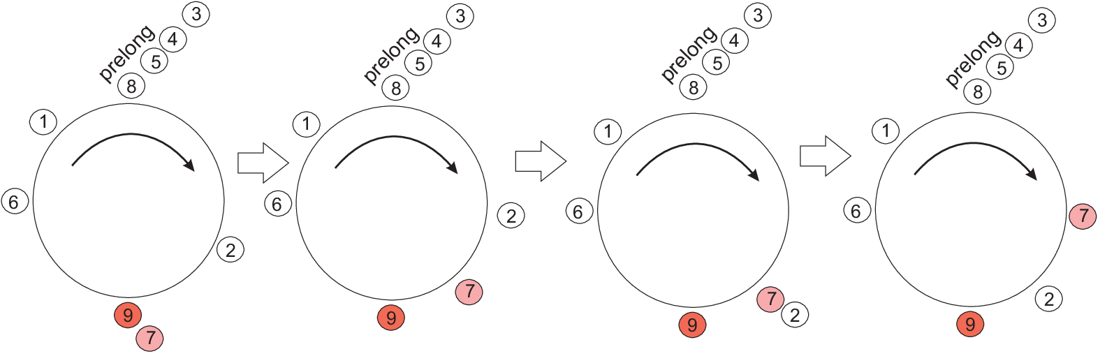
The critical cells that survive path reversing are (See Figure 5):

(1)

All the cells of type 1, and
(2)

All the cells $\big(\spadesuit\ \{k\}I\ \clubsuit\{n,*\}\big)$ of type 2 such that

$k>*,\ \hbox{and}\ k>\clubsuit.$

Proposition 6.2.

The above described path reversing yields a discrete vector field.

Proof. The second axiom of discrete vector field is straightforward. For the first axiom observe that a cell of the complex participates in at most one gradient path that is reversed.∎

We stress once again that unlike reversal of one single path, reversal of several gradient paths does not automatically yield a discrete Morse function. So we have to prove the following proposition.

Proposition 6.3.

The above described discrete vector field is a a discrete Morse function.

Proof. Assume the contrary: there exists a closed path $\Gamma$ . It can be decomposed into some reversed and some unreversed gradient paths between the (former) critical cells. Since a path from type 1 to type 2 never exists, we conclude that all (former) critical cells that appear in $\Gamma$ are of type $2$ . For them there are two possibilities: either (1) all these former critical cells have one and the same entry $k$ preceding the prelong set, or (2) for some of these (former critical) cells the entries preceding the prelong set are different. We treat these cases separately.

(1)

Lemma 5.1 implies that the prelong set is maintained during the path. Therefore no entry greater than $k$ passes through the prelong set. Also no entry smaller than $k$ passes through the $n$ -set. So, no entry makes a full turn.
The closed path $\Gamma$ necessarily includes a reversed path. This means that at some moment, an entry $i$ greater than $k$ comes from $\clubsuit$ and joins the $n$ -set. Consider the consecutive split-step.
1. (a)
  
  If some entry $j$ of the $n$ -set moves forward, it never comes back.
2. (b)
  
  If some entry $j$ of the $n$ -set moves backward, $j$ is necessarily smaller than $k$ , and the entry $j$ never comes back.
(2)

Assume there are different entries right before the prelong sets in this path. Let $j$ be the minimal of these entries. At some step of the path, $j$ leaves the place before the prelong set. The entry $j$ is smaller than the next entry that gets to the place before the prelong set, so it can stay neither in $\spadesuit$ nor in the prelong set. Therefore, $j$ eventually joins the $\clubsuit$ . The only way for $j$ to get back leads through the $n$ -set, where it can get only via some reversed path. Since $j$ is minimal, during that path before the prelong set stands an entry greater than $j$ , which is impossible, according to the reversing condition (3).∎

Theorem 6.4.

The number of critical cells equals the sum of Betti numbers of the manifold $M(L)$ . Consequently, the above described pairing together with path reversal gives a perfect Morse function.

Proof. We know from [4] that each short set containing the entry $n$ contributes ” $2$ ” to the sum of Betti numbers. So, to prove the theorem, we build a bijection between the short sets containing $n$ and pairs of critical cells.

More precisely, we will show that for every short set $J$ consisting of $k+1$ elements and containing the entry $n$ gives exactly one $k$ -cell of type 1, and exactly one $(n-3-k)$ -cell of type 2.

(1)

Cell of type 1. Take $J$ as the $n$ -set of the (uniquely defined) critical cell of type $1$ .

Conversely, each critical cell of type $1$ gives a short set containing $n$ , that is, the $n$ -set.
(2)

Cell of type 2.
1. (a)
  
  Compose a prelong set $I$ . The set $\overline{J}:=[n]\setminus J$ is long. Take the largest entry of $\overline{J}$ and start the prelong set $I$ with it. Keep adding entries from $\overline{J}$ to $I$ in the decreasing order as long as $I$ stays short. The process stops once $I$ becomes prelong (that is, one step before it gets long).
2. (b)
  
  Specify an entry preceding $I$ . Let $j$ be the largest of the $\overline{J}\setminus I$ . Turn $j$ to the singleton that precedes the prelong set $I$ .
3. (c)
  
  Compose an $n$ -set. Define the $n$ -set as $\big(\overline{J}\setminus(I\cup\{j\}\big)\big)\cup\{n\}$ . By construction, each entry in the $n$ -set (except for $n$ ) is smaller than $j$ . Clearly, we get a short set (since the complement is long).
4. (d)
  
  Positions of the rest of the singletons are now defined uniquely. We turn all other entries to singletons, which are placed before $\{j\}$ , if they are larger than $j$ , and after $I$ if they are smaller than $j$ .
Now compute the number of the sets in the partition. All entries of $J$ except $n$ turn to singletons. Moreover, we have a singleton $j$ and two non-singleton sets. Altogether we have $k+3$ sets, so the dimension of the cell is $(n-3-k)$ .

Conversely, each critical cell of type 2 of the new Morse function arises in this way: assume we have a critical cell of type $2$ . Take all the singletons except for the singleton that precedes the prelong set. Add the entry $n$ . Altogether they give the short set containing $n$ associated to the cell.

∎

Two examples

Let $L=(1,1,1,1,1,1,1)$ be the equilateral 7-linkage.

(1)
For the short set $J=\{7\}$ , we have:
1. (a)
  
  The associated cell of type 1 is $\big(\{6\}\ \{5\}\ \{4\}\ \{3\}\ \{2\}\ \{1\}\ \{7\}\big);$
2. (b)
  
  $\overline{J}=\{1,2,3,4,5,6\}$ , $I=\{4,5,6\}$ , $j=3$ , and the associated cell of type 2 is:
  
  $\big(\{3\}\ \{4,5,6\}\ \{7,1,2\}\big)$
(2)
For the short set $J=\{5,6,7\}$ , we have:
1. (a)
  
  The associated cell of type 1 is $\big(\{4\}\ \{3\}\ \{2\}\ \{1\}\ \{7,5,6\}\big);$
2. (b)
  
  $\overline{J}=\{1,2,3,4\}$ , $I=\{2,3,4\}$ , $j=1$ and the associated cell of type 2 is:
  
  $(\{6\}\ \{5\}\ \{1\}\ \{2,3,4\}\ \{7\}\big)$

References

[1] E. Babson, P. Hersh. Discrete Morse functions from lexicographic orders, Trans. AMS, 357, 2 (2005), 509-534.
[2] B. Burton, T. Lewiner, J. Paixëo, J. Spreer, Parameterized complexity of discrete Morse theory, Proceedings of the twenty-ninth annual symposium on Computational geometry. ACM, 2013, 127-136.
[3] M. Farber, Invitation to topological robotics, European Mathematical Society, 2008.
[4] M. Farber, D. Schütz, Homology of planar polygon spaces, Geom. Dedicata, 125 (2007), 75-92.
[5] M. Farber, J.-C. Hausmann, D. Schuetz, On the conjecture of Kevin Walker, Journal of Topology and Analysis, 1 (2009), 65-86.
[6] R. Forman, Morse Theory for Cell Complexes, Adv. in Math. Vol. 134, 1 (1998), 90-145.
[7] R. Forman, A User’s guide to discrete Morse theory, Séminaire Lotharingien de Combinatoire 48 (2002).
[8] P. Hersh, On optimizing discrete Morse functions, Adv. in Applied Mathematics, Vol. 35, 3 (2005) 294-322.
[9] M. Joswig, M. E. Pfetsch, Computing optimal Morse matchings, SIAM J. Discrete Math. 20, (2006), 11-25.
[10] G. Khimshiashvili, G. Panina, On the area of a polygonal linkage, Doklady Mathematics, Vol. 85, 1 (2012), 120-121.
[11] J. Milnor, Lectures on the h-cobordism theorem, Princeton Univ. Press, 1965.
[12] G. Panina, Moduli space of a planar polygonal linkage: a combinatorial description, arXiv:1209.3241

Discrete Morse theory for moduli spaces of flexible polygons, or solitaire game on the circle

Abstract.

Key words and phrases:

1. Introduction

2. Preliminaries

Polygonal linkage: moduli space and the cell complex [12]

Definition 2.1.

Theorem 2.2.

Discrete Morse function on a regular cell complex [6]

3. Pairing on the complex 𝒦\mathcal{K}: ”rules of the game”.

Step 1

Step 2

Step k

Pair search algorithm

Proposition 3.1.

Proof.

4. Critical cells of the complex 𝒦\mathcal{K}

Theorem 4.1.

Proof.

Example 4.2.

Example 4.3.

5. Gradient paths between critical cells

Lemma 5.1.

Proof.

Proposition 5.2.

Proposition 5.3.

Proof.

6. Path reversing: new discrete Morse function

Theorem 6.1.

Path reversing construction.

Proposition 6.2.

Proposition 6.3.

Theorem 6.4.

Two examples

References

3. Pairing on the complex $\mathcal{K}$ : ”rules of the game”.

4. Critical cells of the complex $\mathcal{K}$