跳到论文正文
W Papers独立论文阅读器 arXiv:1504.05087 论文正文 计算阅读时间 · 0%
引用这篇论文根据当前论文元数据生成,正式投稿前建议核对。


License: arXiv.org perpetual non-exclusive license
arXiv:1504.05087v1 [math.ST] 20 Apr 2015

Extreme eigenvalues of large-dimensional spiked Fisher matrices with application

Qinwen Wang    Jianfeng Yao
Abstract

Consider two pp-variate populations, not necessarily Gaussian, with covariance matrices Σ1\Sigma_{1} and Σ2\Sigma_{2}, respectively, and let S1S_{1} and S2S_{2} be the sample covariances matrices from samples of the populations with degrees of freedom TT and nn, respectively. When the difference Δ\Delta between Σ1\Sigma_{1} and Σ2\Sigma_{2} is of small rank compared to p,Tp,T and nn, the Fisher matrix F=S2−1​S1F=S_{2}^{-1}S_{1} is called a spiked Fisher matrix. When p,Tp,T and nn grow to infinity proportionally, we establish a phase transition for the extreme eigenvalues of FF: when the eigenvalues of Δ\Delta (spikes) are above (or under) a critical value, the associated extreme eigenvalues of the Fisher matrix will converge to some point outside the support of the global limit (LSD) of other eigenvalues; otherwise, they will converge to the edge points of the LSD. Furthermore, we derive central limit theorems for these extreme eigenvalues of the spiked Fisher matrix. The limiting distributions are found to be Gaussian if and only if the corresponding population spike eigenvalues in Δ\Delta are simple. Numerical examples are provided to demonstrate the finite sample performance of the results. In addition to classical applications of a Fisher matrix in high-dimensional data analysis, we propose a new method for the detection of signals allowing an arbitrary covariance structure of the noise. Simulation experiments are conducted to illustrate the performance of this detector.

keywords
[class=AMS] Primary 62H12 ; secondary 60F05
keywords
Large-dimensional Fisher matrices , Spiked Fisher matrix , Spiked population model , Extreme eigenvalue , Phase transition , Central limit theorem , Signal detection , high-dimensional data analysis

and

Qinwen Wang
Department of Mathematics
Zhejiang University
??

Jianfeng Yao
Department of Statistics and Actuarial Science
The University of Hong Kong
Pokfulam,   Hong Kong
??

1 Introduction

Consider two pp-variate populations with covariance matrices Σ1\Sigma_{1} and Σ2\Sigma_{2}, respectively, and let S1S_{1} and S2S_{2} be the sample covariances matrices from samples of the populations with degrees of freedom TT and nn, respectively. Specifically, if both populations are Gaussian, T​S1TS_{1} and n​S2nS_{2} are distributed as Wishart WP​(T,Σ1)W_{P}(T,\Sigma_{1}) and WP​(n,Σ2)W_{P}(n,\Sigma_{2}), respectively. For testing the equality hypothesis H0:Σ1=Σ2H_{0}:\penalty\ \Sigma_{1}=\Sigma_{2}, the likelihood ratio statistic relies on the pp characteristic roots of the determinental equation

|S1−l​S2|=0,l∈ℝ.\displaystyle|S_{1}-lS_{2}|=0\penalty\ ,\quad l\in\mathbb{R}. (1.1)

Here and throughout the paper, the determinant of a matrix AA is denoted by either |A||A| or det(A)\det(A). As a famous story in multivariate analysis of last century, the joint distribution of these characteristic roots for Gaussian populations was simultaneously and independently published in 1939 by R. A. Fisher, S. N. Roy, P. L. Hsu and M. A. Girshick. When S2S_{2} is invertible, these roots are simply the eigenvalues of the matrix F=S2−1​S1F=S_{2}^{-1}S_{1}, widely known as a Fisher matrix in the literature, which generalises the one-dimensional Fisher ratio.

Another breakthrough is the work of Wachter (1980) where he finds a deterministic limit, the celebrated Wacheter distribution, for the empirical measure of these roots when the dimension pp grows to infinity proportionally to the degrees of freedom TT and nn (under the Gaussian assumption). Wachter’s result has been later extended to non-Gaussian populations in what is now called the random matrix theory and two early examples of such extensions are Silverstein (1985) and Bai et al. (1987) . It is also important to notice that the determinental equation (1.1) arises not only in the classical hypothesis testing problem mentioned above, it indeed covers also similar equations arising in important fields of multivariate analysis such as discriminant analysis, canonical correlation analysis and MANOVA, see Wachter (1980).

Needless to say that such limiting results allowing large values of dimension pp comparable to the degrees of freedom (i.e. sample sizes) are going to have much impact on today’s high-dimensional data analysis. A particularly important question is to investigate the properties of the characteristic roots under an alternative of form

H1:Σ1=Σ2+Δ,H_{1}:\penalty\ \penalty\ \Sigma_{1}=\Sigma_{2}+\Delta\penalty\ , (1.2)

where Δ\Delta is a nonnegative definite matrix of rank MM. When pp, TT and nn are all large, the discrimination between the null hypothesis and the alternative is not difficult if the rank difference MM is all large. The real challenge here lies in detecting a small rank-MM alternative. In this perspective and assuming MM is a fixed integer while pp, TT and nn grow to infinity proportionally, the empirical measure of the pp characteristic roots of (1.1) will be affected by a difference of order M/pM/p which vanishes, so that its limit remains the same as in the null hypothesis, i.e. the Wachter distribution. In other words, such global limit from all the characteristic roots will be of little help for distinguishing the two hypotheses.

It happens that the useful information to detect a small rank alternative is encoded in a few largest characteristic roots of (1.1). In a recent preprint Dharmawansa et al. (2014), by assuming both population are Gaussian and M=1M=1, these authors show that, when the norm of the rank-1 difference Δ\Delta (spike) exceeds a phase transition threshold, the asymptotic behaviour of the log-ratio of the joint density of these characteristic roots under a local deviation from the spike depends only on the largest characteristic root lp,1l_{p,1} and the statistical experiment of observing all the characteristic roots is locally asymptotically normal (LAN). As a by-product of their analysis, the authors also establish joint asymptotic normality of a few of the largest roots when the corresponding spikes in Δ\Delta (with M>1M>1) exceed the phase transition threshold. As it can be guessed, the analysis given in this reference highly rely on the Gaussian assumption so that the joint density function of the characteristic roots has indeed an explicit form under both the null and the alternative, and the main results are obtained via an accurate analytic approximation of the log-ratio of these density functions when the dimension pp, TT and nn grow to infinity proportionally.

Intrigued by these findings, in this paper, we explore the same questions for general populations without Gaussian assumption. It is thus apparent that the joint density of the characteristic roots no more exist and new techniques are needed to solve the questions. Our approach relies on the tools borrowed from the theory of random matrices. This theory is closely connected to modern high-dimensional statistics, and has provided in recent years many efficient estimation and testing procedures for high-dimensional data analysis. Excellent introduction and surveys on this approach can be found in Bai (2005), Johnstone (2007), Johnstone and Titterington (2009) and Paul and Aue (2014). A methodology particularly successful both in theory and applications within this approach relies on the spiked population model coined in Johnstone (2001). This model deals with one population only with a unit population covariance matrix IpI_{p} and the hypotheses are simply H0:Σ1=IpH_{0}:\Sigma_{1}=I_{p} versus H1:Σ1=Ip+ΔH_{1}:\Sigma_{1}=I_{p}+\Delta where Δ\Delta is a rank-MM difference as in (1.2). Again for small rank MM, the discrimination between both hypotheses will rely on the extreme eigenvalues of the sample covariance matrix S1S_{1}. Important results have been obtained in the last decade on the behaviour of these extreme eigenvalues. For example, the fluctuation of largest eigenvalues of a sample covariance matrix from a complex spiked Gaussian population is studied in Baik et al. (2005). These authors uncover a phase transition phenomenon: the weak limit and the scaling of these extreme eigenvalues are different depending on whether the eigenvalues of Δ\Delta (spikes) are above, equal or below a critical value, situations refereed as super-critical, critical and sub-critical, respectively. In Baik and Silverstein (2006), the authors consider the spiked population model with general populations (not necessarily Gaussian). For the almost sure limits of the extreme sample eigenvalues of S1S_{1}, they find that if a population spike (in Δ\Delta) is large or small enough, the corresponding sample spike eigenvalues will converge to a limit outside the support of the limiting spectrum (outliers). In Paul (2007), a CLT is established for these outliers, i.e. the super-critical case, under the Gaussian assumption and assuming that population spikes are simple (multiplicity 1). The CLT for super-critical outliers with general populations and arbitrary multiplicity numbers is developed in Bai and Yao (2008). This theory has been later extended for generalised spiked population model in Bai and Yao (2012).

In summary, from the perspective of spiked population model, the Fisher matrix F=S2−1​S1F=S_{2}^{-1}S_{1} under the alternative (1.2) can be viewed as a spiked Fisher matrix and it is important to establish a theory for this two-population Fisher matrix FF in the vein of the results discussed above on the one-population spiked covariance matrix S1S_{1}. As said before, in Dharmawansa et al. (2014), the authors have already identified the transition phenomenon for the extreme eigenvalues under the Gaussian assumption, and these eigenvalues are proved to be asymptotic normal assuming that the spike eigenvalues in Δ\Delta are simple. The main contributions of the paper are the following. We prove that this phase transition phenomenon for extreme eigenvalues of a spiked Fisher matrix is universal, valid for general populations under some suitable moment conditions. Next, we provide a general CLT for the extreme sample eigenvalues of FF in the super-critical regime: the limiting distributions are not necessarily Gaussian; they are Gaussian if and only if the population spikes in Δ\Delta are simple.

In addition to the motivations given so far on the importance of a spiked Fisher matrix, we are able to implement an application of the general theory developed in this paper in the context of a signal detection problem with a large number of detectors, see Section 7. Indeed, this problem has its own interests and even with quite limited experiments, we show that our implementation can lead to very reliable solutions.

Finally, within the theory of random matrices, the techniques we use in this paper for spiked models are closely connected to other random matrix ensembles through the concept of small-rank perturbations. The goal is again to examine the effect caused on the extreme sample eigenvalues by such perturbations. Theories on perturbed Wigner matrices can be found in Péché (2006), Féral and Péché (2007), Capitaine et al. (2009), Pizzo et al. (2013) and Renfrew and Soshnikov (2013). In a more general setting of finite-rank perturbation including both the additive and the multiplicative one, point-wisely convergence of extreme eigenvalues is established in Benaych-Georges and Nadakuditi (2011) while their fluctuations are studied in Benaych-Georges et al. (2011). In addition, Benaych-Georges and Nadakuditi (2011) contain also results on spiked eigenvectors.

The rest of the paper is organised as follows. First, the exact setting of the spiked Fisher matrix F=S2−1​S1F=S_{2}^{-1}S_{1} is introduced in Section 2. Then in Section 3, we establish the phase transition phenomenon for the extreme eigenvalues of FF where the transition boundary is explicitly obtained. Next, CLTs for those extreme eigenvalues fluctuating around some outliers (i.e. the super-critical case) are established first in Section 4 for one group of sample eigenvalues corresponding to a same population spike, and then in Section 6 for all the groups jointly. Section 5 contains numerical illustrations that demonstrate the finite sample performance of our results. In Section 7, we develop in details a signal detection technique with prewhitening. Proofs of the main theorems are included in these sections while some technical lemmas are postponed into the Appendix A.

2 Spiked Fisher matrix and preliminary results

In what follows, we will assume that Σ2=Ip\Sigma_{2}=I_{p}. This assumption does not loss any generality since the eigenvalues of the Fisher matrix F=S2−1​S1F=S_{2}^{-1}S_{1} are invariant under the transformation S1↦Σ2−1/2S1Σ2−1/2S_{1}\mapsto\Sigma_{2}^{-1/2}S_{1}\Sigma_{2}^{-1/2}, S2↦Σ2−1/2S2Σ2−1/2S_{2}\mapsto\Sigma_{2}^{-1/2}S_{2}\Sigma_{2}^{-1/2}. Also we will write Σp\Sigma_{p} for Σ1\Sigma_{1} to signify the dependence on the dimension pp. Therefore, the sample covariance matrices S1S_{1} and S2S_{2} that make up the Fisher matrix F=S2−1​S1F=S_{2}^{-1}S_{1} are assumed to have the following structure. Let

Z=(z1,…​zn)=(zi​j)1≤i≤p,1≤j≤n\displaystyle Z=(z_{1},\ldots z_{n})=(z_{ij})_{1\leq i\leq p,1\leq j\leq n} (2.1)

and

W=(w1,…​wT)=(wk​l)1≤k≤p,1≤l≤T\displaystyle W=(w_{1},\ldots w_{T})=(w_{kl})_{1\leq k\leq p,1\leq l\leq T} (2.2)

be two independent arrays, with respective size p×np\times n and p×Tp\times T, of independent real-valued random variables with mean 0 and variance 1. The sample covariance matrix S2S_{2} is

S2=1n​∑j=1nzj​zj∗=1n​Z​Z∗.S_{2}=\frac{1}{n}\sum_{j=1}^{n}z_{j}z_{j}^{*}=\frac{1}{n}ZZ^{*}. (2.3)

Next, Σp\Sigma_{p} is a rank MM perturbation of IpI_{p}; therefore, we can assume that it has the spiked structure of form

Σp=(ΩM00Ip−M),\Sigma_{p}=\left(\begin{array}[]{cc}\Omega_{M}&0\\ 0&I_{p-M}\end{array}\right), (2.4)

where ΩM\Omega_{M} is a M×MM\times M covariance matrix, MM being a fixed constant, containing kk spike eigenvalues (ai)(a_{i}), (a1,⋯,a1⏟n1,⋯,ak,⋯,ak⏟nk)\displaystyle(\underbrace{a_{1},\cdots,a_{1}}_{n_{1}},\cdots,\underbrace{a_{k},\cdots,a_{k}}_{n_{k}}), of respective multiplicity numbers (ni)(n_{i}) (n1+⋯+nk=Mn_{1}+\cdots+n_{k}=M). That is, ΩM=U​diag⁡(a1,⋯,a1,⋯,ak,⋯,ak)​U∗\Omega_{M}=U\mathop{\text{diag}}({a_{1},\cdots,a_{1}},\cdots,{a_{k},\cdots,a_{k}})U^{*}, where UU is a M×MM\times M orthogonal matrix. Consider a sample x1,⋯,xTx_{1},\cdots,x_{T} of size TT that can be expressed as xl:=Σp1/2​wlx_{l}:=\Sigma_{p}^{1/2}w_{l} and let X=(x1,…,XT)=Σp1/2​WX=(x_{1},\ldots,X_{T})=\Sigma_{p}^{1/2}W. The sample covariance matrix S1S_{1} is

S1=1T​∑l=1Txl​xl∗=1T​X​X∗=Σp1/2​(1T​W​W∗)​Σp1/2.S_{1}=\frac{1}{T}\sum_{l=1}^{T}x_{l}x_{l}^{*}=\frac{1}{T}XX^{*}=\Sigma_{p}^{1/2}\left(\frac{1}{T}WW^{*}\right)\Sigma_{p}^{1/2}. (2.5)

Throughout the paper, we consider an asymptotic regime of Marčenko-Pastur type, i.e.

p∧n∧T→∞,yp:=p/n→y∈(0,1),andcp:=p/T→c>0.p\wedge n\wedge T\rightarrow\infty,\quad y_{p}:=p/n\rightarrow y\in(0,1),\quad\text{and}\penalty\ \penalty\ c_{p}:=p/T\rightarrow c>0. (2.6)

Recall that the empirical spectral distribution (ESD) of a p×pp\times p matrix AA with eigenvalues {λj}\{\lambda_{j}\} is the distribution p−1​∑j=1pδλjp^{-1}\sum_{j=1}^{p}\delta_{\lambda_{j}} where δa\delta_{a} denotes the Dirac mass at aa. Since the total rank MM generated by the kk spikes is fixed, the ESD of FF will have the same limit (LSD) as there were no spikes. This limiting spectral distribution, the celebrated Wachter distribution, has been known for a long time.

Proposition 2.1.

For the Fisher matrix F=S2−1​S1F=S_{2}^{-1}S_{1} with the sample covariance matrices SiS_{i}’s given in (2.3)-(2.5), assume that the dimension pp and the two sample sizes n,Tn,T grow to infinity proportionally as in (2.6). Then almost surely, the ESD of FF weakly converges to a deterministic distribution Fc,yF_{c,y} with a bounded support [b1,b][b_{1},b] and a density function given by

fc,y​(x)={(1−y)​(b−x)​(x−b1)2​π​x​(c+x​y),when​b1≤x≤b,0,otherwise,\displaystyle f_{c,y}(x)=\left\{\begin{array}[]{ll}\frac{(1-y)\sqrt{(b-x)(x-b_{1})}}{2\pi x(c+xy)}\penalty\ ,&\quad\text{when}\penalty\ b_{1}\leq x\leq b\penalty\ ,\\ 0\penalty\ ,&\quad\text{otherwise}\penalty\ ,\end{array}\right.

where

b1=(1−c+y−c​y1−y)2andb=(1+c+y−c​y1−y)2.\displaystyle b_{1}=\left(\frac{1-\sqrt{c+y-cy}}{1-y}\right)^{2}\quad\text{and}\quad b=\left(\frac{1+\sqrt{c+y-cy}}{1-y}\right)^{2}. (2.9)

Furthermore, if c>1c>1, then Fc,yF_{c,y} has a point mass 1−1/c1-1/c at the origin. Also, the Stieltjes transform s⁡(z)s(z) of Fc,yF_{c,y} equals:

s⁡(z)=1z​c−1z−c⁡(z⁡(1−y)+1−c)+2​z​y−c​(1−c+z⁡(1−y))2−4​z2​z​c​(c+z​y),z∉[b1,b].\displaystyle s(z)=\frac{1}{zc}-\frac{1}{z}-\frac{c(z(1-y)+1-c)+2zy-c\sqrt{(1-c+z(1-y))^{2}-4z}}{2zc(c+zy)}\penalty\ ,\quad z\notin[b_{1},b]. (2.10)
Remark 2.1.

Assuming both populations are Gaussian, (Wachter, 1980, Theorem 3.1) derives the limiting distribution for roots of the determinental equation ,

|T​S1−x2​(T​S1+n​S2)|=0,x∈ℝ.|TS_{1}-x^{2}(TS_{1}+nS_{2})|=0,\quad x\in\mathbb{R}.

The continuous component of the distribution has a compact support [A2,B2][A^{2},B^{2}] with density function proportional to {(x−A2)​(B2−x)}1/2/{x⁡(1−x2)}\{(x-A^{2})(B^{2}-x)\}^{1/2}/\{x(1-x^{2})\}. It can be readily checked that by the change of variable z=c​x2/{y⁡(1−x2)}z=cx^{2}/\{y(1-x^{2})\}, the density of the continuous component of the LSD of FF is exactly (2.1). The validity of this limit for general populations (non necessarily Gaussian) is due to Silverstein (1985) and Bai et al. (1987).

For a complex number z∉[b1,b]z\notin[b_{1},b], we define the following integrals with respect to Fc,y​(x)F_{c,y}(x):

s⁡(z):=∫1x−z​d​Fc,y​(x),m1​(z):=∫1(z−x)2​d​Fc,y​(x),\displaystyle s(z):=\int\frac{1}{x-z}dF_{c,y}(x)\penalty\ ,\penalty\ \penalty\ \penalty\ \penalty\ \penalty\ \penalty\ \penalty\ m_{1}(z):=\int\frac{1}{(z-x)^{2}}dF_{c,y}(x)\penalty\ ,
m2​(z):=∫xz−x​d​Fc,y​(x),m3​(z):=∫x(z−x)2​d​Fc,y​(x),\displaystyle m_{2}(z):=\int\frac{x}{z-x}dF_{c,y}(x)\penalty\ ,\penalty\ \penalty\ \quad m_{3}(z):=\int\frac{x}{(z-x)^{2}}dF_{c,y}(x)\penalty\ ,
m4​(z):=∫x2(z−x)2​d​Fc,y​(x).\displaystyle m_{4}(z):=\int\frac{x^{2}}{(z-x)^{2}}dF_{c,y}(x)\penalty\ . (2.11)

3 Phase transition of the extreme eigenvalues of F=S2−1​S1F=S_{2}^{-1}S_{1}

In this section, we establish a phase transition phenomenon for the extreme eigenvalues of F=S2−1​S1F=S_{2}^{-1}S_{1}, that is, when a population spike aia_{i} with multiplicity nin_{i} is larger (or smaller) than a critical value, a packet of nin_{i} corresponding sample eigenvalues of FF will jump outside the support [b1,b][b_{1},b] of its LSD Fc,yF_{c,y} and converge all to a fixed limit. Otherwise, these associated sample eigenvalues will converge to one of the edges b1b_{1} and bb.

For notation convenience, let γ=1/(1−y)∈(1,∞)\gamma=1/(1-y)\in(1,\infty). Define the function

ϕ⁡(x)=γ​x​(x−1+c)x−γ,x≠γ,\phi(x)=\frac{\gamma x(x-1+c)}{x-\gamma},\quad x\neq\gamma, (3.1)

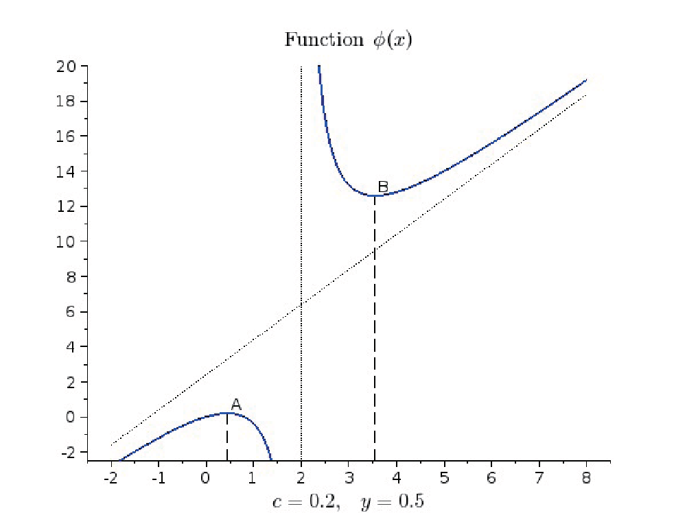
which is a rational function with a single pole γ\gamma. An example is depicted in Figure 1 with parameters (c,y)=(15,12)(c,y)=(\frac{1}{5},\frac{1}{2}). The function has an asymptote of equation g⁡(x)=γ⁡(x+c−1+γ)g(x)=\gamma(x+c-1+\gamma) when |x|→∞|x|\to\infty.

Refer to caption
Figure 1: Example of the ϕ\phi function with (c,y)=(15,12)(c,y)=(\frac{1}{5},\frac{1}{2}) and pole γ=2\gamma=2. The asymptote has equation y=2​x+125y=2x+\frac{12}{5}. The boundary points are A⁡(0.450,0.203)A(0.450,0.203) and B⁡(3.549,12.597)B(3.549,12.597) meaning that critical values for spikes are 0.450 and 3.549 while the support of the LSD is [0.203,12.597].

By assumption, the kk population spike eigenvalues {ai}\{a_{i}\} are all positive and non unit. We order them with their multiplicities in descending order together with the p−Mp-M unit eigenvalues as

a1=⋯=a1>a2=⋯=a2>⋯>ak0=⋯=ak0>1=⋯=1>\displaystyle a_{1}=\cdots=a_{1}>a_{2}=\cdots=a_{2}>\cdots>a_{k_{0}}=\cdots=a_{k_{0}}>1=\cdots=1>
ak0+1=⋯=ak0+1>⋯>ak=⋯=ak.\displaystyle\quad a_{k_{0}+1}=\cdots=a_{k_{0}+1}>\cdots>a_{k}=\cdots=a_{k}. (3.2)

That is, k0k_{0} of these spike eigenvalues are larger than 1 while the other k−k0k-k_{0} are smaller. Let

Ji={[n1+⋯+ni−1+1,n1+⋯+ni],1≤i≤k0,[p−(ni+⋯+nk)+1,,p−(ni+1+⋯+nk)],k0<i≤k.\displaystyle J_{i}=\begin{cases}[n_{1}+\cdots+n_{i-1}+1,n_{1}+\cdots+n_{i}]\penalty\ ,&\quad 1\leq i\leq k_{0}\penalty\ ,\\ [p-(n_{i}+\cdots+n_{k})+1,,p-(n_{i+1}+\cdots+n_{k})]\penalty\ ,&\quad k_{0}<i\leq k\penalty\ .\end{cases}

Notice that the cardinality of each JiJ_{i} is nin_{i}. Next, the sample eigenvalues {lp,j}\{l_{p,j}\} of the Fisher matrix S2−1​S1S_{2}^{-1}S_{1} are also sorted in the descending order as lp,1≥lp,2≥⋯≥lp,pl_{p,1}\geq l_{p,2}\geq\cdots\geq l_{p,p}. Therefore, for each spike eigenvalue aia_{i}, there are nin_{i} associated sample eigenvalues {lp,j,j∈Ji}\{l_{p,j},\penalty\ j\in J_{i}\}.

Theorem 3.1.

For the Fisher matrix F=S2−1​S1F=S_{2}^{-1}S_{1} with the sample covariance matrices SiS_{i}’s given in (2.3)-(2.5), assume that the dimension pp and the two sample sizes n,Tn,T grow to infinity proportionally as in (2.6). Then for any spike eigenvalue aia_{i} (i=1,⋯,ki=1,\cdots,k), it holds that for all j∈Jij\in J_{i}, lp,jl_{p,j} almost surely converges to a limit

λi={ϕ⁡(ai),|ai−γ|>γ​c+y−c​y,b,1<ai≤γ⁡{1+c+y−c​y},b1,γ⁡{1−c+y−c​y}≤ai<1.\displaystyle\lambda_{i}=\begin{cases}\phi(a_{i}),&\quad|a_{i}-\gamma|>\gamma\sqrt{c+y-cy}\penalty\ ,\\ b,&\quad 1<a_{i}\leq\gamma\{1+\sqrt{c+y-cy}\}\penalty\ ,\\ b_{1},&\quad\gamma\{1-\sqrt{c+y-cy}\}\leq a_{i}<1\penalty\ .\end{cases} (3.3)

Basically, the theorem establishes a phase transition phenomenon for the largest and smallest sample eigenvalues of a Fisher matrix. Consider again the example shown in Figure 1. The transition boundary is indicated with the boundary points AA and BB with respective coordinates

A⁡(γ⁡{1−c+y−c​y},b1)andB⁡(γ⁡{1+c+y−c​y},b).A(\gamma\{1-\sqrt{c+y-cy}\},b_{1})\quad\text{and}\quad B(\gamma\{1+\sqrt{c+y-cy}\},b).

When the spike is large enough or small enough, the corresponding sample eigenvalues converge to ϕ⁡(ai)\phi(a_{i}) located outside the support [b1,b][b_{1},b] of the LSD of FF. Otherwise, they converge to one of its edges b1b_{1} and bb.

It is worth observing that when y→0y\to 0, the ϕ⁡(x)\phi(x) function tends to the function well-known in the literature for similar transition phenomenon of a spiked sample covariance matrix, i.e.

limy→0ϕ⁡(x)=x+c​xx−1,x≠1,\displaystyle\lim_{y\to 0}\phi(x)=x+\frac{cx}{x-1},\quad x\neq 1, (3.4)

see e.g. the ψ\psi-function on Figure 4 of Bai and Yao (2012). These functions share a same shape; however the pole here equals γ=1/(1−y)\gamma=1/(1-y) which is larger than the pole 1 for the case of a spiked sample covariance matrix.

As said in Introduction, this transition phenomenon has already been established in a preprint Dharmawansa et al. (2014) (their Proposition 5) under Gaussian assumption and using a completely different approach. Theorem 3.1 proves that such a phase transition phenomenon is indeed universal.

Proof.

(of Theorem 3.1) The proof is divided into the following three steps:

  • •

    Step 1: we derive the almost sure limit of an outlier eigenvalue of S2−1​S1S_{2}^{-1}S_{1};

  • •

    Step 2: we show that in order for the extreme eigenvalue of S2−1​S1S_{2}^{-1}S_{1} to be an outlier, the population spike aia_{i} should be larger (or smaller) than a critical value;

  • •

    Step 3: if not so, the extreme eigenvalue of S2−1​S1S_{2}^{-1}S_{1} will converge to one of the edge points bb and b1b_{1}.

Step 1: Let lp,j​(j∈Ji)l_{p,j}\penalty\ (j\in J_{i}) be the outlier eigenvalue of S2−1​S1S_{2}^{-1}S_{1} corresponding to the population spike aia_{i}. Then lp,jl_{p,j} must satisfy the following equation:

|lp,j​Ip−S2−1​S1|=0,\displaystyle|l_{p,j}I_{p}-S_{2}^{-1}S_{1}|=0\penalty\ ,

and it is equivalent to

|lp,j​S2−S1|=0.\displaystyle|l_{p,j}S_{2}-S_{1}|=0\penalty\ . (3.5)

Now we make some short-hands. Denote Z=(Z1Z2)Z=\left(\begin{array}[]{c}Z_{1}\\ Z_{2}\end{array}\right), where Z1Z_{1} is the nn observations of its first MM coordinates and Z2Z_{2} the remaining. We partition XX accordingly as X=(X1X2),X=\left(\begin{array}[]{c}X_{1}\\ X_{2}\end{array}\right), where X1X_{1} is the TT observations of its first MM coordinates and X2X_{2} the remaining. Using such a representation, we have

S1=1T​X​X∗=1T​(X1​X1∗X1​X2∗X2​X1∗X2​X2∗),S2=1n​Z​Z∗=1n​(Z1​Z1∗Z1​Z2∗Z2​Z1∗Z2​Z2∗).\displaystyle S_{1}=\frac{1}{T}XX^{*}=\frac{1}{T}\left(\begin{array}[]{cc}X_{1}X^{*}_{1}&X_{1}X^{*}_{2}\\[5.69054pt] X_{2}X^{*}_{1}&X_{2}X^{*}_{2}\end{array}\right),\quad S_{2}=\frac{1}{n}ZZ^{*}=\frac{1}{n}\left(\begin{array}[]{cc}Z_{1}Z^{*}_{1}&Z_{1}Z^{*}_{2}\\[5.69054pt] Z_{2}Z^{*}_{1}&Z_{2}Z^{*}_{2}\end{array}\right)\penalty\ .

Then, (3.5) could be written in the block form:

|(lp,jn​Z1​Z1∗−1T​X1​X1∗lp,jn​Z1​Z2∗−1T​X1​X2∗lp,jn​Z2​Z1∗−1T​X2​X1∗lp,jn​Z2​Z2∗−1T​X2​X2∗)|=0.\displaystyle\left|\left(\begin{array}[]{cc}\frac{l_{p,j}}{n}Z_{1}Z^{*}_{1}-\frac{1}{T}X_{1}X^{*}_{1}&\frac{l_{p,j}}{n}Z_{1}Z^{*}_{2}-\frac{1}{T}X_{1}X^{*}_{2}\\[5.69054pt] \frac{l_{p,j}}{n}Z_{2}Z^{*}_{1}-\frac{1}{T}X_{2}X^{*}_{1}&\frac{l_{p,j}}{n}Z_{2}Z^{*}_{2}-\frac{1}{T}X_{2}X^{*}_{2}\end{array}\right)\right|=0\penalty\ .

Since lp,jl_{p,j} is an outlier, it holds |lp,j⋅1n​Z2​Z2∗−1T​X2​X2∗|≠0|l_{p,j}\cdot\frac{1}{n}Z_{2}Z^{*}_{2}-\frac{1}{T}X_{2}X^{*}_{2}|\neq 0, and for block matrix, we have det(ABCD)=detD⋅det(A−B​D−1​C)\det\begin{pmatrix}A&B\\ C&D\\ \end{pmatrix}=\det D\cdot\det(A-BD^{-1}C) when DD is invertible. Therefore, (3) reduces to

|lp,jnZ1Z∗1−1TX1X∗1\displaystyle\left|\frac{l_{p,j}}{n}Z_{1}Z^{*}_{1}-\frac{1}{T}X_{1}X^{*}_{1}\right.
−(lp,jnZ1Z2∗−1TX1X2∗)(lp,jnZ2Z2∗−1TX2X2∗)−1(lp,jnZ2Z1∗−1TX2X1∗)|=0.\displaystyle\quad-\left.\Big(\frac{l_{p,j}}{n}Z_{1}Z^{*}_{2}-\frac{1}{T}X_{1}X^{*}_{2}\Big)\Big(\frac{l_{p,j}}{n}Z_{2}Z^{*}_{2}-\frac{1}{T}X_{2}X^{*}_{2}\Big)^{-1}\Big(\frac{l_{p,j}}{n}Z_{2}Z^{*}_{1}-\frac{1}{T}X_{2}X^{*}_{1}\Big)\right|=0\penalty\ .

More specifically, we have

det(lp,jn​Z1​[In−Z2∗​(lp,j​Ip−(1n​Z2​Z2∗)−1​1T​X2​X2∗)−1​(1n​Z2​Z2∗)−1​lp,jn​Z2]​Z1∗⏟(I)CLOSE\displaystyle\det\bigg(\underbrace{\frac{l_{p,j}}{n}Z_{1}\Big[I_{n}-Z^{*}_{2}\big(l_{p,j}I_{p}-(\frac{1}{n}Z_{2}Z^{*}_{2})^{-1}\frac{1}{T}X_{2}X^{*}_{2}\big)^{-1}(\frac{1}{n}Z_{2}Z^{*}_{2})^{-1}\frac{l_{p,j}}{n}Z_{2}\Big]Z^{*}_{1}}_{(I)}
−1T​X1​[IT+X2∗​(lp,j​Ip−(1n​Z2​Z2∗)−1​1T​X2​X2∗)−1​(1n​Z2​Z2∗)−1​1T​X2]​X1∗⏟(I​I)\displaystyle\underbrace{-\frac{1}{T}X_{1}\Big[I_{T}+X^{*}_{2}\big(l_{p,j}I_{p}-(\frac{1}{n}Z_{2}Z^{*}_{2})^{-1}\frac{1}{T}X_{2}X^{*}_{2}\big)^{-1}(\frac{1}{n}Z_{2}Z^{*}_{2})^{-1}\frac{1}{T}X_{2}\Big]X^{*}_{1}}_{(II)}
+lp,jn​Z1​Z2∗​(lp,j​Ip−(1n​Z2​Z2∗)−1​1T​X2​X2∗)−1​(1n​Z2​Z2∗)−1​1T​X2​X1∗⏟(I​I​I)\displaystyle+\underbrace{\frac{l_{p,j}}{n}Z_{1}Z^{*}_{2}\big(l_{p,j}I_{p}-(\frac{1}{n}Z_{2}Z^{*}_{2})^{-1}\frac{1}{T}X_{2}X^{*}_{2}\big)^{-1}(\frac{1}{n}Z_{2}Z^{*}_{2})^{-1}\frac{1}{T}X_{2}X^{*}_{1}}_{(III)}
OPEN+1T​X1​X2∗​(lp,j​Ip−(1n​Z2​Z2∗)−1​1T​X2​X2∗)−1​(1n​Z2​Z2∗)−1​lp,jn​Z2​Z1∗⏟(I​V))\displaystyle+\underbrace{\frac{1}{T}X_{1}X^{*}_{2}\big(l_{p,j}I_{p}-(\frac{1}{n}Z_{2}Z^{*}_{2})^{-1}\frac{1}{T}X_{2}X^{*}_{2}\big)^{-1}(\frac{1}{n}Z_{2}Z^{*}_{2})^{-1}\frac{l_{p,j}}{n}Z_{2}Z^{*}_{1}}_{(IV)}\bigg)
=0.\displaystyle=0\penalty\ . (3.12)

In all the following, we denote by SS the Fisher matrix (1n​Z2​Z2∗)−1​1T​X2​X2∗\left(\frac{1}{n}Z_{2}Z^{*}_{2}\right)^{-1}\frac{1}{T}X_{2}X^{*}_{2}, which has a LSD Fc,y​(x)F_{c,y}(x). And in order to find the limit of lp,jl_{p,j}, we simply find the limit on the left hand side of (3.12), then it will generate an equation. Solving this equation will give the value of its limit.

First, consider the terms (I​I​I)(III) and (I​V)(IV). Since (Z1,X1)(Z_{1},X_{1}) is independent of (Z2,X2)(Z_{2},X_{2}), using Lemma A.2, we see these two terms will converge to some constant multiplied by the covariance matrix between X1X_{1} and Z1Z_{1}. On the other hand, X1X_{1} is also independent of Z1Z_{1}, we have

Cov​(X1,Z1)=𝔼​X1​Z1−𝔼​X1​𝔼​Z1=𝔼​X1​𝔼​Z1−𝔼​X1​𝔼​Z1=𝟎M×M.\displaystyle\text{Cov}(X_{1},Z_{1})=\mathbb{E}X_{1}Z_{1}-\mathbb{E}X_{1}\mathbb{E}Z_{1}=\mathbb{E}X_{1}\mathbb{E}Z_{1}-\mathbb{E}X_{1}\mathbb{E}Z_{1}={\bf 0}_{M\times M}\penalty\ .

Therefore, these two terms will both tend to a zero matrix 𝟎M×M{\bf 0}_{M\times M} almost surely.

So the remaining task is to find the limit of (I)(I) and (I​I)(II). We recall the expression of X1X_{1} and Z1Z_{1} that

Cov​(X1)=U​diag⁡(a1,⋯,a1⏟n1,⋯,ak,⋯,ak⏟nk)​U∗,Cov​(Z1)=IM.\displaystyle\text{Cov}(X_{1})=U\mathop{\text{diag}}(\underbrace{a_{1},\cdots,a_{1}}_{n_{1}},\cdots,\underbrace{a_{k},\cdots,a_{k}}_{n_{k}})U^{*}\penalty\ ,\quad\text{Cov}(Z_{1})=I_{M}.

According to Lemma A.2, we have

(I)\displaystyle(I) =lp,jn​Z1​[In−Z2∗​(lp,j​Ip−S)−1​(1n​Z2​Z2∗)−1​lp,jn​Z2]​Z1∗\displaystyle=\frac{l_{p,j}}{n}Z_{1}\bigg[I_{n}-Z^{*}_{2}(l_{p,j}I_{p}-S)^{-1}(\frac{1}{n}Z_{2}Z^{*}_{2})^{-1}\frac{l_{p,j}}{n}Z_{2}\bigg]Z^{*}_{1}
→λin​{𝔼​tr⁡[In−Z2∗​(λi​Ip−S)−1​(1n​Z2​Z2∗)−1​λin​Z2]}⋅IM\displaystyle\rightarrow\frac{\lambda_{i}}{n}\left\{\mathbb{E}\mathop{\text{tr}}\bigg[I_{n}-Z^{*}_{2}(\lambda_{i}I_{p}-S)^{-1}(\frac{1}{n}Z_{2}Z^{*}_{2})^{-1}\frac{\lambda_{i}}{n}Z_{2}\bigg]\right\}\cdot I_{M}
=λi​(1+y​λi​s​(λi))⋅IM,\displaystyle=\lambda_{i}(1+y\lambda_{i}s(\lambda_{i}))\cdot I_{M}\penalty\ , (3.13)

here, we denote λi\lambda_{i} as the limit of the outlier {lp,j,j∈Ji}\left\{l_{p,j},j\in J_{i}\right\}. For the same reason,

(I​I)\displaystyle(II) =−1T​X1​[IT+X2∗​(lp,j​Ip−S)−1​(1n​Z2​Z2∗)−1​1T​X2]​X1∗\displaystyle=-\frac{1}{T}X_{1}\bigg[I_{T}+X^{*}_{2}(l_{p,j}I_{p}-S)^{-1}(\frac{1}{n}Z_{2}Z^{*}_{2})^{-1}\frac{1}{T}X_{2}\bigg]X^{*}_{1}
→−1T{𝔼tr[IT+X2∗(λiIp−S)−1(1nZ2Z2∗)−11TX2]}⋅U(a1⋱ak)U∗\displaystyle\rightarrow-\frac{1}{T}\left\{\mathbb{E}\mathop{\text{tr}}\bigg[I_{T}+X^{*}_{2}(\lambda_{i}I_{p}-S)^{-1}(\frac{1}{n}Z_{2}Z^{*}_{2})^{-1}\frac{1}{T}X_{2}\bigg]\right\}\cdot U\left(\begin{array}[]{c}a_{1}\\ \penalty\ \ddots\\ \qquad a_{k}\end{array}\right)U^{*}
=U⁡(−1+c+c​λi​s​(λi))⋅(a1⋱ak)​U∗.\displaystyle=U\big(-1+c+c\lambda_{i}s(\lambda_{i})\big)\cdot\left(\begin{array}[]{c}a_{1}\\ \penalty\ \ddots\\ \qquad a_{k}\end{array}\right)U^{*}\penalty\ .

Therefore, combining (3.12), (3.13) and (3), we have the determinant of the following M×MM\times M matrix

U​(λi​(1+y​λi​s​(λi))+(−1+c+c​λi​s​(λi))​a10⋮⋱⋮0λi​(1+y​λi​s​(λi))+(−1+c+c​λi​s​(λi))​ak)​U∗\displaystyle U\begin{pmatrix}\lambda_{i}(1+y\lambda_{i}s(\lambda_{i}))+(-1+c+c\lambda_{i}s(\lambda_{i}))a_{1}\quad\quad\quad 0\\ \vdots\quad\quad\quad\quad\quad\quad\quad\quad\ddots\quad\quad\quad\quad\quad\quad\quad\quad\quad\vdots\\ \quad\quad\quad 0\quad\quad\quad\lambda_{i}(1+y\lambda_{i}s(\lambda_{i}))+(-1+c+c\lambda_{i}s(\lambda_{i}))a_{k}&\\ \end{pmatrix}U^{*}

equal to zero, which is also to say that λi\lambda_{i} satisfies the equation:

λi​(1+y​λi​s​(λi))+(−1+c+c​λi​s​(λi))​ai=0.\displaystyle\lambda_{i}(1+y\lambda_{i}s(\lambda_{i}))+(-1+c+c\lambda_{i}s(\lambda_{i}))a_{i}=0\penalty\ . (3.20)

Finally, together with the expression of the Stieltjes transform of a Fisher matrix in (2.10), we have

λi=ai​(ai+c−1)ai−ai​y−1=ϕ⁡(ai),\displaystyle\lambda_{i}=\frac{a_{i}(a_{i}+c-1)}{a_{i}-a_{i}y-1}=\phi(a_{i})\penalty\ ,

where the function ϕ⁡(x)\phi(x) is defined in (3.4).

Step 2: Define s¯​(z)\underline{s}(z) as the Stieltjes transform of the LSD of 1T​X2∗​(1n​Z2​Z2∗)−1​X2\frac{1}{T}X^{*}_{2}(\frac{1}{n}Z_{2}Z^{*}_{2})^{-1}X_{2}, who shares the same non-zero eigenvalues as S2−1​S1S_{2}^{-1}S_{1}. Then we have the relationship:

s¯​(z)+1z​(1−c)=c​s​(z).\displaystyle\underline{s}(z)+\frac{1}{z}(1-c)=cs(z)\penalty\ . (3.21)

Recall the expression of s⁡(z)s(z) in (2.10), we have

s¯​(z)=−c⁡(z⁡(1−y)+1−c)+2​z​y−c​(1−c+z⁡(1−y))2−4​z2​z​(c+z​y).\displaystyle\underline{s}(z)=-\frac{c(z(1-y)+1-c)+2zy-c\sqrt{(1-c+z(1-y))^{2}-4z}}{2z(c+zy)}\penalty\ . (3.22)

On the other hand, due to (3.20) and (3.21), we have the value for s¯​(λi)\underline{s}(\lambda_{i}):

s¯​(λi)=y​c−y−cy​λi+ai​c.\displaystyle\underline{s}(\lambda_{i})=\frac{yc-y-c}{y\lambda_{i}+a_{i}c}\penalty\ . (3.23)

Since λi\lambda_{i} is outside the support of the LSD, we have

s¯−1​(y​c−y−cy​λi+ai​c)=λi>bors¯−1​(y​c−y−cy​λi+ai​c)=λi<b1\displaystyle\underline{s}^{-1}\left(\frac{yc-y-c}{y\lambda_{i}+a_{i}c}\right)=\lambda_{i}>b\quad\text{or}\quad\underline{s}^{-1}\left(\frac{yc-y-c}{y\lambda_{i}+a_{i}c}\right)=\lambda_{i}<b_{1}\penalty\

which is also to say that

s¯​(b)<y​c−y−cy​λi+ai​c,\displaystyle\underline{s}(b)<\frac{yc-y-c}{y\lambda_{i}+a_{i}c}\penalty\ , (3.24)

or

s¯​(b1)>y​c−y−cy​λi+ai​c.\displaystyle\underline{s}(b_{1})>\frac{yc-y-c}{y\lambda_{i}+a_{i}c}\penalty\ . (3.25)

Then (3.24) says that s¯​(b)\underline{s}(b) must be smaller than the minimum value on its right hand side, whose minimum value is attained when λi=b\lambda_{i}=b (the right hand side of (3.24) is a decreasing function of λi\lambda_{i}). Similarly, (3.25) says that s¯​(b1)\underline{s}(b_{1}) must be larger than the maximum value on its right hand side, which is attained when λi=b1\lambda_{i}=b_{1}. Therefore, the condition for λi\lambda_{i} be an outlier is:

s¯​(b)<y​c−y−cy​b+ai​c,ors¯​(b1)>y​c−y−cy​b1+ai​c.\displaystyle\underline{s}(b)<\frac{yc-y-c}{yb+a_{i}c},\quad\text{or}\quad\underline{s}(b_{1})>\frac{yc-y-c}{yb_{1}+a_{i}c}. (3.26)

Finally, using (3.22) together with the value of bb and b1b_{1}, we have:

ai>1+c+y−c​y1−y,orai<1−c+y−c​y1−y,\displaystyle a_{i}>\frac{1+\sqrt{c+y-cy}}{1-y},\penalty\ \quad\text{or}\quad a_{i}<\frac{1-\sqrt{c+y-cy}}{1-y},

which is equivalent to say that (recall the expression of γ\gamma that γ=1/(1−y)\gamma=1/(1-y)):

|ai−γ|>γ​c+y−c​y.\displaystyle|a_{i}-\gamma|>\gamma\sqrt{c+y-cy}\penalty\ .

Step 3: In this step, we show that if the condition in Step 2 is not fulfilled, then the extreme eigenvalues of S2−1​S1S_{2}^{-1}S_{1} will tend to one of the edge points b1b_{1} and bb. For simplicity, we only show the convergence to the right edge bb: the proof for the convergence to the left edge b1b_{1} is similar. Thus suppose all the ai>1a_{i}>1 for i=1,⋯,ki=1,\cdots,k. For now, we make some short-hands. Let

S1=1T​X​X∗=1T​(X1​X1∗X1​X2∗X2​X1∗X2​X2∗):=(B11B12B21B22)\displaystyle S_{1}=\frac{1}{T}XX^{*}=\frac{1}{T}\left(\begin{array}[]{cc}X_{1}X^{*}_{1}&X_{1}X^{*}_{2}\\[5.69054pt] X_{2}X^{*}_{1}&X_{2}X^{*}_{2}\end{array}\right):=\begin{pmatrix}B_{11}&B_{12}\\ B_{21}&B_{22}\\ \end{pmatrix}

and

S2=1n​Z​Z∗=1n​(Z1​Z1∗Z1​Z2∗Z2​Z1∗Z2​Z2∗):=(A11A12A21A22),\displaystyle S_{2}=\frac{1}{n}ZZ^{*}=\frac{1}{n}\left(\begin{array}[]{cc}Z_{1}Z^{*}_{1}&Z_{1}Z^{*}_{2}\\[5.69054pt] Z_{2}Z^{*}_{1}&Z_{2}Z^{*}_{2}\end{array}\right):=\begin{pmatrix}A_{11}&A_{12}\\ A_{21}&A_{22}\\ \end{pmatrix}\penalty\ ,

where B11B_{11} and A11A_{11} are the corresponding blocks with size M×MM\times M. Using the inverse formula for block matrix, the (p−M)×(p−M)(p-M)\times(p-M) major sub-matrix of S2−1​S1S^{-1}_{2}S_{1} is

−(A22−A21​A11−1​A12)−1​A21​A11−1​B12+(A22−A21​A11−1​A12)−1​B22:=C.\displaystyle-(A_{22}-A_{21}A^{-1}_{11}A_{12})^{-1}A_{21}A^{-1}_{11}B_{12}+(A_{22}-A_{21}A^{-1}_{11}A_{12})^{-1}B_{22}:=C\penalty\ . (3.27)

The part

−(A22−A21A11−1A12)−1A21A11−1B12=−(A22−A21A11−1A12)−1A21A11−1⋅1TX1X2∗\displaystyle-(A_{22}-A_{21}A^{-1}_{11}A_{12})^{-1}A_{21}A^{-1}_{11}B_{12}=-(A_{22}-A_{21}A^{-1}_{11}A_{12})^{-1}A_{21}A^{-1}_{11}\cdot\frac{1}{T}X_{1}X^{*}_{2}

is of rank MM; besides, we have

tr⁡{(A22−A21​A11−1​A12)−1​A21​A11−1​1T​X1​X2∗}→0,\displaystyle\mathop{\text{tr}}\left\{(A_{22}-A_{21}A^{-1}_{11}A_{12})^{-1}A_{21}A^{-1}_{11}\frac{1}{T}X_{1}X^{*}_{2}\right\}\rightarrow 0\penalty\ ,

since X1X_{1} is independent of X2X_{2}. Therefore, the MM nonzero eigenvalues of the matrix −(A22−A21​A11−1​A12)−1​A21​A11−1​B12-(A_{22}-A_{21}A^{-1}_{11}A_{12})^{-1}A_{21}A^{-1}_{11}B_{12} will all tend to zero (so is its largest one). Then consider the second part of (3.27) as follows.

A22−A21​A11−1​A12=1n​Z2​[In−Z1∗​(1n​Z1​Z1∗)−1​1n​Z1]​Z2∗:=1n​Z2​P​Z2.\displaystyle A_{22}-A_{21}A^{-1}_{11}A_{12}=\frac{1}{n}Z_{2}\left[I_{n}-Z^{*}_{1}\big(\frac{1}{n}Z_{1}Z^{*}_{1}\big)^{-1}\frac{1}{n}Z_{1}\right]Z^{*}_{2}:=\frac{1}{n}Z_{2}PZ_{2}\penalty\ .

Since P=In−Z1∗​(1n​Z1​Z1∗)−1​1n​Z1P=I_{n}-Z^{*}_{1}\big(\frac{1}{n}Z_{1}Z^{*}_{1}\big)^{-1}\frac{1}{n}Z_{1} is a projection matrix of rank p−Mp-M, it has the spectral decomposition:

P=V⁡(0⋱0In−M)​V∗,\displaystyle P=V\left(\begin{array}[]{cccc}0&&&\\ &\ddots&&\\ &&0&\\ &&&{I}_{n-M}\\ \end{array}\right)V^{*}\penalty\ ,

where VV is a n×nn\times n orthogonal matrix. Since MM is fixed, the ESD of PP tends to δ1\delta_{1}, which leads to the fact that the LSD of the matrix 1n​Z2​P​Z2∗\frac{1}{n}Z_{2}PZ^{*}_{2} is the standard Marčenko-Pastur law. Then the matrix (1n​Z2​P​Z2∗)−1​B22(\frac{1}{n}Z_{2}PZ^{*}_{2})^{-1}B_{22} is a standard Fisher matrix, and its largest eigenvalues (finitely many) will tend to the right edge bb of the Wachter distribution. It follows then the two largest eigenvalues of CC, say α1​(C)\alpha_{1}(C) and α2​(C)\alpha_{2}(C), also tend to bb.

Next since CC is the (p−M)×(p−M)(p-M)\times(p-M) major sub-matrix of S2−1​S1S^{-1}_{2}S_{1}, we have by Cauchy interlacing theorem

α2​(C)≤lp,M+1≤α1​(C)≤lp,1.\alpha_{2}(C)\leq l_{p,M+1}\leq\alpha_{1}(C)\leq l_{p,1}\penalty\ .

Thus lp,M+1→bl_{p,M+1}\to b either. On the other hand, we have

lp,1=‖S2−1​S1‖o​p≤‖S2−1‖o​p⋅‖S1‖o​p,\displaystyle l_{p,1}=\|S^{-1}_{2}S_{1}\|_{op}\leq\|S_{2}^{-1}\|_{op}\cdot\|S_{1}\|_{op},

so that for some positive constant θ\theta, lim suplp,1≤θ\limsup l_{p,1}\leq\theta. Consequently, almost surely,

b≤lim inflp,M≤⋯≤lim suplp,1≤θ<∞;b\leq\liminf l_{p,M}\leq\cdots\leq\limsup l_{p,1}\leq\theta<\infty\penalty\ ;

in particular the whole family {lp,j, 1≤j≤M}\{l_{p,j},\penalty\ 1\leq j\leq M\} is bounded. Now let 1≤j≤M1\leq j\leq M be fixed and assume that a subsequence (lpk,j)k(l_{p_{k},j})_{k} converges to a limit β∈[b,θ]\beta\in[b,\theta]. Either β=ϕ⁡(ai)>b\beta=\phi(a_{i})>b or β=b\beta=b. However, according to Step 2, β>b\beta>b implies that ai>γ⁡{1+c+y−c​y}a_{i}>\gamma\{1+\sqrt{c+y-cy}\}, and otherwise, we have ai≤γ⁡{1+c+y−c​y}a_{i}\leq\gamma\{1+\sqrt{c+y-cy}\}. Therefore, accordingly to one of these two conditions, all subsequences converge to a same limit ϕ⁡(ai)\phi(a_{i}) or bb, which is thus also the unique limit of the whole sequence (lp,j)p(l_{p,j})_{p}.

The proof of Theorem 3.1 is complete. ∎

4 Central limit theorem for the outlier eigenvalues of S2−1​S1S^{-1}_{2}S_{1}

The aim of this section is to give a CLT for the nin_{i}-packed outlier eigenvalues:

p​{lp,j−ϕ⁡(ai),j∈Ji}.\displaystyle\sqrt{p}\penalty\ \{l_{p,j}-\phi(a_{i}),j\in J_{i}\}\penalty\ .

Denote U=(U1U2⋯Uk),U=\begin{pmatrix}U_{1}&U_{2}&\cdots&U_{k}\\ \end{pmatrix}\penalty\ , where each UiU_{i} is a M×niM\times n_{i} matrix that corresponds to the nin_{i}-packed spike eigenvalue aia_{i}.

Theorem 4.1.

Assume the same assumptions as in Theorem 3.1 and in addition, the variables (zi​j)(z_{ij}) (in (2.1)) and (wk​l)(w_{kl}) (in (2.2)) have the same first four moments and denote v4v_{4} as their common fourth moment:

v4=𝔼​|zi​j|4=𝔼​|wk​l|4,1≤i,k≤p, 1≤j≤n, 1≤l≤T.v_{4}=\mathbb{E}|z_{ij}|^{4}=\mathbb{E}|w_{kl}|^{4},\quad 1\leq i,k\leq p,\penalty\ 1\leq j\leq n,\penalty\ 1\leq l\leq T.

Then for any population spike aia_{i} satisfying |ai−γ|>γ​c+y−c​y|a_{i}-\gamma|>\gamma\sqrt{c+y-cy}, the normalised nin_{i}-packed outlier eigenvalues of S2−1​S1S_{2}^{-1}S_{1}: p​{lp,j−ϕ⁡(ai),j∈Ji}\sqrt{p}\penalty\ \{l_{p,j}-\phi(a_{i}),j\in J_{i}\} converge weakly to the distribution of the eigenvalues of the random matrix −Ui∗R(λi)Ui/Δ(λi)-U^{*}_{i}R(\lambda_{i})U_{i}/\Delta(\lambda_{i}). Here,

Δ⁡(λi)=(1−ai−c)​(1+ai​(y−1))2(ai−1)​(−1+2​ai+c+ai2​(y−1)),\displaystyle\Delta(\lambda_{i})=\frac{(1-a_{i}-c)(1+a_{i}(y-1))^{2}}{(a_{i}-1)(-1+2a_{i}+c+a_{i}^{2}(y-1))}\penalty\ , (4.1)

R⁡(λi)=(Rm​n)R(\lambda_{i})=(R_{mn}) is a M×MM\times M symmetric random matrix, made with independent Gaussian entries of mean zero and variance

𝕍​ar​(Rm​n)={2​θi+(v4−3)​ωi,m=n,θi,m≠n,\displaystyle\mathbb{V\text{ar}}(R_{mn})=\left\{\begin{array}[]{ll}2\theta_{i}+(v_{4}-3)\omega_{i}\penalty\ ,&m=n\penalty\ ,\\ \theta_{i}\penalty\ ,&m\neq n\penalty\ ,\end{array}\right.

where

ωi=ai2​(ai+c−1)2​(c+y)(ai−1)2,\displaystyle\omega_{i}=\frac{a_{i}^{2}(a_{i}+c-1)^{2}(c+y)}{(a_{i}-1)^{2}}\penalty\ , (4.4)
θi=ai2​(ai+c−1)2​(c​y−c−y)−1+2​ai+c+ai2​(y−1).\displaystyle\theta_{i}=\frac{a_{i}^{2}(a_{i}+c-1)^{2}(cy-c-y)}{-1+2a_{i}+c+a_{i}^{2}(y-1)}\penalty\ . (4.5)

Numerical illustrations of this theorem are detailed in the next section.

Remark 4.1.

Notice that the result above involves the ii-th block UiU_{i} of the eigen-matrix UU. When the spike aia_{i} is simple, UiU_{i} is unique up to its sign, then Ui∗​R​(λi)​UiU^{*}_{i}R(\lambda_{i})U_{i} is uniquely determined. But when aia_{i} has multiplicities greater than 1, UiU_{i} is not unique; actually, any rotation of UiU_{i} can be an eigenvector matrix corresponding to aia_{i}. Therefore, Lemma A.1 in the Appendix states that, such a rotation will not affect the eigenvalues of the matrix Ui∗​R​(λi)​UiU^{*}_{i}R(\lambda_{i})U_{i}.

Proof.

(proof of Theorem 4.1)

Step 1: Convergence to the eigenvalues of the random matrix −Ui∗R(λi)Ui/Δ(λi)-U^{*}_{i}R(\lambda_{i})U_{i}/\Delta(\lambda_{i}). We start from (3.12). First we make some short hands. Define

A⁡(λ)\displaystyle A(\lambda) =In−Z2∗​[λ​Ip−(1n​Z2​Z2∗)−1​1T​X2​X2∗]−1​(1n​Z2​Z2∗)−1​λn​Z2,\displaystyle=I_{n}-Z^{*}_{2}\bigg[\lambda I_{p}-\Big(\frac{1}{n}Z_{2}Z^{*}_{2}\Big)^{-1}\frac{1}{T}X_{2}X^{*}_{2}\bigg]^{-1}\Big(\frac{1}{n}Z_{2}Z^{*}_{2}\Big)^{-1}\frac{\lambda}{n}Z_{2}\penalty\ ,
B⁡(λ)\displaystyle B(\lambda) =IT+X2∗​[λ​Ip−(1n​Z2​Z2∗)−1​1T​X2​X2∗]−1​(1n​Z2​Z2∗)−1​1T​X2,\displaystyle=I_{T}+X^{*}_{2}\bigg[\lambda I_{p}-\Big(\frac{1}{n}Z_{2}Z^{*}_{2}\Big)^{-1}\frac{1}{T}X_{2}X^{*}_{2}\bigg]^{-1}\Big(\frac{1}{n}Z_{2}Z^{*}_{2}\Big)^{-1}\frac{1}{T}X_{2}\penalty\ ,
C⁡(λ)\displaystyle C(\lambda) =Z2∗​[λ​Ip−(1n​Z2​Z2∗)−1​1T​X2​X2∗]−1​(1n​Z2​Z2∗)−1​1T​X2,\displaystyle=Z^{*}_{2}\bigg[\lambda I_{p}-\Big(\frac{1}{n}Z_{2}Z^{*}_{2}\Big)^{-1}\frac{1}{T}X_{2}X^{*}_{2}\bigg]^{-1}\Big(\frac{1}{n}Z_{2}Z^{*}_{2}\Big)^{-1}\frac{1}{T}X_{2}\penalty\ ,
D⁡(λ)\displaystyle D(\lambda) =X2∗​[λ​Ip−(1n​Z2​Z2∗)−1​1T​X2​X2∗]−1​(1n​Z2​Z2∗)−1​1n​Z2,\displaystyle=X^{*}_{2}\bigg[\lambda I_{p}-\Big(\frac{1}{n}Z_{2}Z^{*}_{2}\Big)^{-1}\frac{1}{T}X_{2}X^{*}_{2}\bigg]^{-1}\Big(\frac{1}{n}Z_{2}Z^{*}_{2}\Big)^{-1}\frac{1}{n}Z_{2}\penalty\ , (4.6)

then (3.12) could be written as

det(lp,jn​Z1​A​(lp,j)​Z1∗⏟(i)−1T​X1​B​(lp,j)​X1∗⏟(i​i)+lp,jn​Z1​C​(lp,j)​X1∗⏟(i​i​i)+lp,jT​X1​D​(lp,j)​Z1∗⏟(i​v))=0.\displaystyle\det\bigg(\underbrace{\frac{l_{p,j}}{n}Z_{1}A(l_{p,j})Z^{*}_{1}}_{(i)}-\underbrace{\frac{1}{T}X_{1}B(l_{p,j})X^{*}_{1}}_{(ii)}+\underbrace{\frac{l_{p,j}}{n}Z_{1}C(l_{p,j})X^{*}_{1}}_{(iii)}+\underbrace{\frac{l_{p,j}}{T}X_{1}D(l_{p,j})Z^{*}_{1}}_{(iv)}\bigg)=0\penalty\ . (4.7)

The remaining is to find second order approximation of the four terms on the left hand side of (4.7).

Using Lemma A.5 in the appendix, we have

(i)\displaystyle(i) =𝔼​λin​Z1​A​(λi)​Z1∗+lp,jn​Z1​A​(lp,j)​Z1∗−𝔼​λin​Z1​A​(λi)​Z1∗\displaystyle=\mathbb{E}\frac{\lambda_{i}}{n}Z_{1}A(\lambda_{i})Z^{*}_{1}+\frac{l_{p,j}}{n}Z_{1}A(l_{p,j})Z^{*}_{1}-\mathbb{E}\frac{\lambda_{i}}{n}Z_{1}A(\lambda_{i})Z^{*}_{1}
=(λi+y​λi2​s​(λi))⋅IM+lp,jn​Z1​A​(lp,j)​Z1∗−λin​Z1​A​(λi)​Z1∗+λin​Z1​A​(λi)​Z1∗−𝔼​λin​Z1​A​(λi)​Z1∗\displaystyle=(\lambda_{i}+y\lambda_{i}^{2}s(\lambda_{i}))\cdot I_{M}+\frac{l_{p,j}}{n}Z_{1}A(l_{p,j})Z^{*}_{1}-\frac{\lambda_{i}}{n}Z_{1}A(\lambda_{i})Z^{*}_{1}+\frac{\lambda_{i}}{n}Z_{1}A(\lambda_{i})Z^{*}_{1}-\mathbb{E}\frac{\lambda_{i}}{n}Z_{1}A(\lambda_{i})Z^{*}_{1}
=(λi+y​λi2​s​(λi))⋅IM+lp,j−λin​Z1​A​(lp,j)​Z1∗+λin​Z1​(A⁡(lp,j)−A⁡(λi))​Z1∗\displaystyle=(\lambda_{i}+y\lambda_{i}^{2}s(\lambda_{i}))\cdot I_{M}+\frac{l_{p,j}-\lambda_{i}}{n}Z_{1}A(l_{p,j})Z^{*}_{1}+\frac{\lambda_{i}}{n}Z_{1}\left(A(l_{p,j})-A(\lambda_{i})\right)Z^{*}_{1}
+λin​[1n​Z1​A​(λi)​Z1∗−𝔼​1n​Z1​A​(λi)​Z1∗]\displaystyle\quad+\frac{\lambda_{i}}{\sqrt{n}}\Big[\frac{1}{\sqrt{n}}Z_{1}A(\lambda_{i})Z^{*}_{1}-\mathbb{E}\frac{1}{\sqrt{n}}Z_{1}A(\lambda_{i})Z^{*}_{1}\Big]
→(λi+y​λi2​s​(λi))⋅IM+(lp,j−λi)⋅(1+2​y​λi​s​(λi)+λi2​y​m1​(λi))⋅IM\displaystyle\rightarrow(\lambda_{i}+y\lambda_{i}^{2}s(\lambda_{i}))\cdot I_{M}+(l_{p,j}-\lambda_{i})\cdot(1+2y\lambda_{i}s(\lambda_{i})+\lambda_{i}^{2}ym_{1}(\lambda_{i}))\cdot I_{M}
+λin​[1n​Z1​A​(λi)​Z1∗−𝔼​1n​Z1​A​(λi)​Z1∗],\displaystyle\quad+\frac{\lambda_{i}}{\sqrt{n}}\Big[\frac{1}{\sqrt{n}}Z_{1}A(\lambda_{i})Z^{*}_{1}-\mathbb{E}\frac{1}{\sqrt{n}}Z_{1}A(\lambda_{i})Z^{*}_{1}\Big]\penalty\ , (4.8)
(i​i)\displaystyle(ii) =𝔼​1T​X1​B​(λi)​X1∗+1T​X1​B​(lp,j)​X1∗−𝔼​1T​X1​B​(λi)​X1∗\displaystyle=\mathbb{E}\frac{1}{T}X_{1}B(\lambda_{i})X^{*}_{1}+\frac{1}{T}X_{1}B(l_{p,j})X^{*}_{1}-\mathbb{E}\frac{1}{T}X_{1}B(\lambda_{i})X^{*}_{1}
=U⁡(1−c−c​λi​s​(λi))⋅(a1⋱ak)​U∗+1T​X1​(B⁡(lp,j)−B⁡(λi))​X1∗\displaystyle=U\big(1-c-c\lambda_{i}s(\lambda_{i})\big)\cdot\left(\begin{array}[]{c}a_{1}\\ \penalty\ \ddots\\ \qquad a_{k}\\ \end{array}\right)U^{*}+\frac{1}{T}X_{1}(B(l_{p,j})-B(\lambda_{i}))X^{*}_{1}
+1T​[1T​X1​B​(λi)​X1∗−𝔼​1T​X1​B​(λi)​X1∗]\displaystyle\quad+\frac{1}{\sqrt{T}}\Big[\frac{1}{\sqrt{T}}X_{1}B(\lambda_{i})X^{*}_{1}-\mathbb{E}\frac{1}{\sqrt{T}}X_{1}B(\lambda_{i})X^{*}_{1}\Big]
→U⁡(1−c−c​λi​s​(λi))⋅(a1⋱ak)​U∗−U⁡(lp,j−λi)⋅c​m3​(λi)⋅(a1⋱ak)​U∗\displaystyle\rightarrow U\big(1-c-c\lambda_{i}s(\lambda_{i})\big)\cdot\left(\begin{array}[]{c}a_{1}\\ \penalty\ \ddots\\ \qquad a_{k}\\ \end{array}\right)U^{*}-U(l_{p,j}-\lambda_{i})\cdot cm_{3}(\lambda_{i})\cdot\left(\begin{array}[]{c}a_{1}\\ \penalty\ \ddots\\ \qquad a_{k}\\ \end{array}\right)U^{*}
+1T​[1T​X1​B​(λi)​X1∗−𝔼​1T​X1​B​(λi)​X1∗],\displaystyle\quad+\frac{1}{\sqrt{T}}\Big[\frac{1}{\sqrt{T}}X_{1}B(\lambda_{i})X^{*}_{1}-\mathbb{E}\frac{1}{\sqrt{T}}X_{1}B(\lambda_{i})X^{*}_{1}\Big]\penalty\ , (4.18)
(i​i​i)\displaystyle(iii) =lp,jn​Z1​C​(lp,j)​X1∗−𝔼​λin​Z1​C​(λi)​X1∗\displaystyle=\frac{l_{p,j}}{n}Z_{1}C(l_{p,j})X^{*}_{1}-\mathbb{E}\frac{\lambda_{i}}{n}Z_{1}C(\lambda_{i})X^{*}_{1}
=lp,jn​Z1​C​(lp,j)​X1∗−λin​Z1​C​(λi)​X1∗+λin​Z1​C​(λi)​X1∗−𝔼​λin​Z1​C​(λi)​X1∗\displaystyle=\frac{l_{p,j}}{n}Z_{1}C(l_{p,j})X^{*}_{1}-\frac{\lambda_{i}}{n}Z_{1}C(\lambda_{i})X^{*}_{1}+\frac{\lambda_{i}}{n}Z_{1}C(\lambda_{i})X^{*}_{1}-\mathbb{E}\frac{\lambda_{i}}{n}Z_{1}C(\lambda_{i})X^{*}_{1}
=lp,jn​Z1​(C⁡(lp,j)−C⁡(λi))​X1∗+lp,j−λin​Z1​C​(λi)​X1∗+λin⋅[Z1​C​(λi)​X1∗−𝔼​Z1​C​(λi)​X1∗]\displaystyle=\frac{l_{p,j}}{n}Z_{1}(C(l_{p,j})-C(\lambda_{i}))X^{*}_{1}+\frac{l_{p,j}-\lambda_{i}}{n}Z_{1}C(\lambda_{i})X^{*}_{1}+\frac{\lambda_{i}}{n}\cdot\Big[Z_{1}C(\lambda_{i})X^{*}_{1}-\mathbb{E}Z_{1}C(\lambda_{i})X^{*}_{1}\Big]
→λin⋅[Z1​C​(λi)​X1∗−𝔼​Z1​C​(λi)​X1∗],\displaystyle\rightarrow\frac{\lambda_{i}}{n}\cdot\Big[Z_{1}C(\lambda_{i})X^{*}_{1}-\mathbb{E}Z_{1}C(\lambda_{i})X^{*}_{1}\Big]\penalty\ , (4.19)
(i​v)\displaystyle(iv) =lp,jT​X1​D​(lp,j)​Z1∗−𝔼​λiT​X1​D​(λi)​Z1∗\displaystyle=\frac{l_{p,j}}{T}X_{1}D(l_{p,j})Z^{*}_{1}-\mathbb{E}\frac{\lambda_{i}}{T}X_{1}D(\lambda_{i})Z^{*}_{1}
=lp,jT​X1​D​(lp,j)​Z1∗−λiT​X1​D​(λi)​Z1∗+λiT​X1​D​(λi)​Z1∗−𝔼​λiT​X1​D​(λi)​Z1∗\displaystyle=\frac{l_{p,j}}{T}X_{1}D(l_{p,j})Z^{*}_{1}-\frac{\lambda_{i}}{T}X_{1}D(\lambda_{i})Z^{*}_{1}+\frac{\lambda_{i}}{T}X_{1}D(\lambda_{i})Z^{*}_{1}-\mathbb{E}\frac{\lambda_{i}}{T}X_{1}D(\lambda_{i})Z^{*}_{1}
=lp,jT​X1​(D⁡(lp,j)−D⁡(λi))​Z1∗+lp,j−λiT​X1​D​(λi)​Z1∗+λiT⋅[X1​D​(λi)​Z1∗−𝔼​X1​D​(λi)​Z1∗]\displaystyle=\frac{l_{p,j}}{T}X_{1}(D(l_{p,j})-D(\lambda_{i}))Z^{*}_{1}+\frac{l_{p,j}-\lambda_{i}}{T}X_{1}D(\lambda_{i})Z^{*}_{1}+\frac{\lambda_{i}}{T}\cdot\Big[X_{1}D(\lambda_{i})Z^{*}_{1}-\mathbb{E}X_{1}D(\lambda_{i})Z^{*}_{1}\Big]
→λiT⋅[X1​D​(λi)​Z1∗−𝔼​X1​D​(λi)​Z1∗].\displaystyle\rightarrow\frac{\lambda_{i}}{T}\cdot\Big[X_{1}D(\lambda_{i})Z^{*}_{1}-\mathbb{E}X_{1}D(\lambda_{i})Z^{*}_{1}\Big]\penalty\ . (4.20)

Denote

Rn​(λi)\displaystyle R_{n}(\lambda_{i}) =λi​pn​[1n​Z1​A​(λi)​Z1∗]−pT​[1T​X1​B​(λi)​X1∗]+λi​pn​[1n​Z1​C​(λi)​X1∗]\displaystyle=\lambda_{i}\sqrt{\frac{p}{n}}\bigg[\frac{1}{\sqrt{n}}Z_{1}A(\lambda_{i})Z^{*}_{1}\bigg]-\sqrt{\frac{p}{T}}\bigg[\frac{1}{\sqrt{T}}X_{1}B(\lambda_{i})X^{*}_{1}\bigg]+\lambda_{i}\sqrt{\frac{p}{n}}\bigg[\frac{1}{\sqrt{n}}Z_{1}C(\lambda_{i})X^{*}_{1}\bigg]
+λi​pT​[1T​X1​D​(λi)​Z1∗]−𝔼⁡[⋅],\displaystyle\quad+\lambda_{i}\sqrt{\frac{p}{T}}\bigg[\frac{1}{\sqrt{T}}X_{1}D(\lambda_{i})Z^{*}_{1}\bigg]-\mathbb{E}[\cdot]\penalty\ , (4.21)

where 𝔼⁡[⋅]\mathbb{E}[\cdot] denotes the total expectation of all the preceding terms in the equation, and

Δ⁡(λi)\displaystyle\Delta(\lambda_{i}) =1+2​y​λi​s​(λi)+λi2​y​m1​(λi)+a​c​m3​(λi).\displaystyle=1+2y\lambda_{i}s(\lambda_{i})+\lambda_{i}^{2}ym_{1}(\lambda_{i})+acm_{3}(\lambda_{i})\penalty\ .

Combining (4.7), (4.8), (4.18), (4.19), (4.20) and considering the diagonal block that corresponds to the row and column index in Ji×JiJ_{i}\times J_{i} leads to:

|p​(lp,j−λi)⋅Δ⁡(λi)⋅Ini+[U∗​Rn​(λi)​U]i|→0.\displaystyle\Big|\sqrt{p}(l_{p,j}-\lambda_{i})\cdot\Delta(\lambda_{i})\cdot I_{n_{i}}+[U^{*}R_{n}(\lambda_{i})U]_{i}\Big|\rightarrow 0\penalty\ . (4.22)

Furthermore, it will be established in Step 2 below that

[U∗​Rn​(λi)​U]i⟶[U∗​R​(λi)​U]iin distribution,[U^{*}R_{n}(\lambda_{i})U]_{i}\longrightarrow[U^{*}R(\lambda_{i})U]_{i}\quad\text{in distribution}, (4.23)

for some random matrix R⁡(λi)R(\lambda_{i}). Using the device of Skorokhod strong representation (Skorokhod, 1956; Hu and Bai, 2014), we may assume that this convergence hold almost surely by considering an enlarged probability space. Under this device, (4.22) is equivalent to say that p​(lp,j−λi)\sqrt{p}(l_{p,j}-\lambda_{i}) tends to an eigenvalue of the matrix −[U∗R(λi)U]i/Δ(λi)(=−Ui∗R(λi)Ui/Δ(λi))-[U^{*}R(\lambda_{i})U]_{i}/\Delta(\lambda_{i})(=-U^{*}_{i}R(\lambda_{i})U_{i}/\Delta(\lambda_{i})). Finally, as the index jj is arbitrary over the set JiJ_{i}, all the nin_{i} random variables

{p​(lp,j−λi),j∈Ji}\displaystyle\left\{\sqrt{p}(l_{p,j}-\lambda_{i}),j\in J_{i}\right\}

converge almost surely to the set of eigenvalues of the random matrix −Ui∗R(λi)Ui/Δ(λi)-U^{*}_{i}R(\lambda_{i})U_{i}/\Delta(\lambda_{i}). Besides, due to Lemma A.3, we have

Δ⁡(λi)\displaystyle\Delta(\lambda_{i}) =1+2​y​λi​s​(λi)+λi2​y​m1​(λi)+a​c​m3​(λi)\displaystyle=1+2y\lambda_{i}s(\lambda_{i})+\lambda_{i}^{2}ym_{1}(\lambda_{i})+acm_{3}(\lambda_{i})
=(1−ai−c)​(1+ai​(y−1))2(ai−1)​(−1+2​ai+c+ai2​(y−1)).\displaystyle=\frac{(1-a_{i}-c)(1+a_{i}(y-1))^{2}}{(a_{i}-1)(-1+2a_{i}+c+a_{i}^{2}(y-1))}\penalty\ .

Step 2: Proof of the convergence (4.23) and structure of the random matrix R⁡(λi)R(\lambda_{i}). In the second step, we aim to find the matrix limit of the block random matrix [U∗​Rn​(λi)​U]i[U^{*}R_{n}(\lambda_{i})U]_{i}. First, we show [U∗​Rn​(λi)​U]i[U^{*}R_{n}(\lambda_{i})U]_{i} equals to another random matrix [U∗​R~n​(λi)​U]i[U^{*}\tilde{R}_{n}(\lambda_{i})U]_{i}, here R~n​(λi)\tilde{R}_{n}(\lambda_{i}) is the type of random sesquilinear form. Then using the results in Bai and Yao (2008) (Proposition 3.1 and Remark 1), we are able to find the matrix limit of R~n​(λi)\tilde{R}_{n}(\lambda_{i}).

By assumption (b) that xi=Σp1/2​six_{i}=\Sigma^{1/2}_{p}s_{i}, we have its first MM components

X1=Ωp1/2​S1=U⁡(a1⋱ak)​U∗​S1.\displaystyle X_{1}=\Omega^{1/2}_{p}S_{1}=U\left(\begin{array}[]{c}\sqrt{a_{1}}\\ \penalty\ \ddots\\ \qquad\sqrt{a_{k}}\end{array}\right)U^{*}S_{1}\penalty\ .

Recall the definition of Rn​(λi)R_{n}(\lambda_{i}) in (4.21), we have

U∗​Rn​(λi)​U\displaystyle\quad\penalty\ U^{*}R_{n}(\lambda_{i})U
=U∗​p​λin​Z1​A​(λi)​Z1∗​U−pT​(a1⋱ak)​U∗​S1​B​(λi)​S1∗​U​(a1⋱ak)\displaystyle=U^{*}\frac{\sqrt{p}\lambda_{i}}{n}Z_{1}A(\lambda_{i})Z^{*}_{1}U-\frac{\sqrt{p}}{T}\left(\begin{array}[]{c}\sqrt{a_{1}}\\ \penalty\ \ddots\\ \qquad\sqrt{a_{k}}\end{array}\right)U^{*}S_{1}B(\lambda_{i})S^{*}_{1}U\left(\begin{array}[]{c}\sqrt{a_{1}}\\ \penalty\ \ddots\\ \qquad\sqrt{a_{k}}\end{array}\right)
+U∗​p​λin​Z1​C​(λi)​S1∗​U​(a1⋱ak)+λi​pT​(a1⋱ak)​U∗​S1​D​(λi)​Z1∗​U\displaystyle\quad+U^{*}\frac{\sqrt{p}\lambda_{i}}{n}Z_{1}C(\lambda_{i})S^{*}_{1}U\left(\begin{array}[]{c}\sqrt{a_{1}}\\ \penalty\ \ddots\\ \qquad\sqrt{a_{k}}\end{array}\right)+\frac{\lambda_{i}\sqrt{p}}{T}\left(\begin{array}[]{c}\sqrt{a_{1}}\\ \penalty\ \ddots\\ \qquad\sqrt{a_{k}}\end{array}\right)U^{*}S_{1}D(\lambda_{i})Z^{*}_{1}U
−𝔼⁡[⋅].\displaystyle\quad-\mathbb{E}[\cdot]\penalty\ . (4.36)

Therefore, if we consider its ii-th block that corresponds to the row and column index in the set Ji×JiJ_{i}\times J_{i}:

[U∗​Rn​(λi)​U]i\displaystyle\quad\penalty\ [U^{*}R_{n}(\lambda_{i})U]_{i}
=λi​pn​[1n​U∗​Z1​A​(λi)​Z1∗​U]i−ai​pT​[1T​U∗​S1​B​(λi)​S1∗​U]i\displaystyle=\lambda_{i}\sqrt{\frac{p}{n}}\Big[\frac{1}{\sqrt{n}}U^{*}Z_{1}A(\lambda_{i})Z^{*}_{1}U\Big]_{i}-a_{i}\sqrt{\frac{p}{T}}\Big[\frac{1}{\sqrt{T}}U^{*}S_{1}B(\lambda_{i})S^{*}_{1}U\Big]_{i}
+λi​ai​pn​[1n​U∗​Z1​C​(λi)​S1∗​U]i+λi​ai​pT​[1T​U∗​S1​D​(λi)​Z1∗​U]i\displaystyle\quad+\lambda_{i}\sqrt{a_{i}}\sqrt{\frac{p}{n}}\Big[\frac{1}{\sqrt{n}}U^{*}Z_{1}C(\lambda_{i})S^{*}_{1}U\Big]_{i}+\lambda_{i}\sqrt{a_{i}}\sqrt{\frac{p}{T}}\Big[\frac{1}{\sqrt{T}}U^{*}S_{1}D(\lambda_{i})Z^{*}_{1}U\Big]_{i}
−𝔼⁡[⋅]\displaystyle\quad-\mathbb{E}[\cdot]
=[λipnU∗Z1A(λi)Z1∗U−aipTU∗S1B(λi)S1∗U\displaystyle=\Big[\lambda_{i}\frac{\sqrt{p}}{n}U^{*}Z_{1}A(\lambda_{i})Z^{*}_{1}U-a_{i}\frac{\sqrt{p}}{T}U^{*}S_{1}B(\lambda_{i})S^{*}_{1}U
+λiaipnU∗Z1C(λi)S1∗U+λiaipTU∗S1D(λi)Z1∗U]i\displaystyle\quad+\lambda_{i}\sqrt{a_{i}}\frac{\sqrt{p}}{n}U^{*}Z_{1}C(\lambda_{i})S^{*}_{1}U+\lambda_{i}\sqrt{a_{i}}\frac{\sqrt{p}}{T}U^{*}S_{1}D(\lambda_{i})Z^{*}_{1}U\Big]_{i}
−𝔼⁡[⋅]\displaystyle\quad-\mathbb{E}[\cdot]
=[U∗​(Z1S1)​(λi​p​A​(λi)nλi​ai​p​C​(λi)nλi​ai​p​D​(λi)T−ai​p​B​(λi)T)​(Z1∗S1∗)​U−𝔼⁡[⋅]]i\displaystyle=\left[U^{*}\begin{pmatrix}Z_{1}&S_{1}\\ \end{pmatrix}\left(\begin{array}[]{cc}\frac{\lambda_{i}\sqrt{p}A(\lambda_{i})}{n}&\frac{\lambda_{i}\sqrt{a_{i}p}C(\lambda_{i})}{n}\\[5.69054pt] \frac{\lambda_{i}\sqrt{a_{i}p}D(\lambda_{i})}{T}&\frac{-a_{i}\sqrt{p}B(\lambda_{i})}{T}\end{array}\right)\begin{pmatrix}Z^{*}_{1}\\[8.53581pt] S^{*}_{1}\\ \end{pmatrix}U-\mathbb{E}[\cdot]\right]_{i}
:=[U∗​R~n​(λi)​U]i\displaystyle:=[U^{*}\tilde{R}_{n}(\lambda_{i})U]_{i}
=Ui∗​R~n​(λi)​Ui,\displaystyle=U^{*}_{i}\tilde{R}_{n}(\lambda_{i})U_{i}\penalty\ , (4.39)

where

R~n​(λi):=(Z1S1)​(λi​p​A​(λi)nλi​ai​p​C​(λi)nλi​ai​p​D​(λi)T−ai​p​B​(λi)T)​(Z1∗S1∗)−𝔼⁡[⋅].\displaystyle\tilde{R}_{n}(\lambda_{i}):=\begin{pmatrix}Z_{1}&S_{1}\\ \end{pmatrix}\left(\begin{array}[]{cc}\frac{\lambda_{i}\sqrt{p}A(\lambda_{i})}{n}&\frac{\lambda_{i}\sqrt{a_{i}p}C(\lambda_{i})}{n}\\[5.69054pt] \frac{\lambda_{i}\sqrt{a_{i}p}D(\lambda_{i})}{T}&\frac{-a_{i}\sqrt{p}B(\lambda_{i})}{T}\end{array}\right)\begin{pmatrix}Z^{*}_{1}\\[8.53581pt] S^{*}_{1}\\ \end{pmatrix}-\mathbb{E}[\cdot]\penalty\ .

Finally, using Lemma A.6 in the appendix leads to the result. The proof of Theorem 4.1 is complete. ∎

Next we consider a special case where Ωp\Omega_{p} is diagonal, whose eigenvalues being all simple. In other words, we have M=kM=k and ni=1n_{i}=1 for all 1≤i≤M1\leq i\leq M. Hence U=IMU=I_{M}. Following Theorem 4.1, we can derive the asymptotic normality for the normalised outlier eigenvalues of S2−1​S1S^{-1}_{2}S_{1} when |ai−γ|>γ​c+y−c​y|a_{i}-\gamma|>\gamma\sqrt{c+y-cy}.

Proposition 4.1.

Under the same assumptions as in Theorem 3.1, with additional conditions that Ωp\Omega_{p} is diagonal and all its eigenvalues aia_{i} (1≤i≤M1\leq i\leq M) are simple, we have when |ai−γ|>γ​c+y−c​y|a_{i}-\gamma|>\gamma\sqrt{c+y-cy}, the outlier eigenvalue lil_{i} of S2−1​S1S_{2}^{-1}S_{1} is asymptotically Gaussian:

p​(li−ai​(ai−1+c)ai−1−ai​y)⟹N⁡(0,σi2),\displaystyle\sqrt{p}\penalty\ \left(l_{i}-\frac{a_{i}(a_{i}-1+c)}{a_{i}-1-a_{i}y}\right)\Longrightarrow N(0,\sigma^{2}_{i})\penalty\ ,

where

σi2\displaystyle\sigma^{2}_{i} =2​ai2​(c​y−c−y)​(ai−1)2​(−1+2​ai+c+ai2​(y−1))(1+ai​(y−1))4\displaystyle=\frac{2a^{2}_{i}(cy-c-y)(a_{i}-1)^{2}(-1+2a_{i}+c+a^{2}_{i}(y-1))}{(1+a_{i}(y-1))^{4}}
+(v4−3)⋅ai2​(c+y)​(−1+2​ai+c+ai2​(y−1))2(1+ai​(y−1))4.\displaystyle\quad+(v_{4}-3)\cdot\frac{a^{2}_{i}(c+y)(-1+2a_{i}+c+a^{2}_{i}(y-1))^{2}}{(1+a_{i}(y-1))^{4}}\penalty\ .
Remark 4.2.

Notice that when the data are standard Gaussian, we have v4=3v_{4}=3, then the above theorem reduces to

p​(li−ai​(ai−1+c)ai−1−ai​y)\displaystyle\sqrt{p}\left(l_{i}-\frac{a_{i}(a_{i}-1+c)}{a_{i}-1-a_{i}y}\right)
⟹N⁡(0,2​ai2​(ai−1)2​(c​y−c−y)​(−1+2​ai+c+ai2​(y−1))(1+ai​(y−1))4),\displaystyle\Longrightarrow N\left(0,\frac{2a_{i}^{2}(a_{i}-1)^{2}(cy-c-y)(-1+2a_{i}+c+a_{i}^{2}(y-1))}{(1+a_{i}(y-1))^{4}}\right)\penalty\ ,

which is exactly the result in Dharmawansa et al. (2014), see setting 1 in their Proposition 11.

Proof.

(of Proposition 4.1) Under the above assumptions, the random matrix −[U∗​R​(λi)​U]i-[U^{*}R(\lambda_{i})U]_{i} reduces to −[R⁡(λi)]i-[R(\lambda_{i})]_{i}. And since all the ni=1n_{i}=1, we have −[R⁡(λi)]i-[R(\lambda_{i})]_{i} equals the (i,i)(i,i)-th element of −R⁡(λi)-R(\lambda_{i}), which is a Gaussian random variable with mean zero and variance

2​θi+(v4−3)​ωi=2​ai2​(ai+c−1)2​(c​y−c−y)−1+2​ai+c+ai2​(y−1)+(v4−3)⋅ai2​(ai+c−1)2​(c+y)(ai−1)2.\displaystyle 2\theta_{i}+(v_{4}-3)\omega_{i}=\frac{2a_{i}^{2}(a_{i}+c-1)^{2}(cy-c-y)}{-1+2a_{i}+c+a_{i}^{2}(y-1)}+(v_{4}-3)\cdot\frac{a_{i}^{2}(a_{i}+c-1)^{2}(c+y)}{(a_{i}-1)^{2}}.

Therefore, combining with (4.1) we have

p​(li−ai​(ai−1+c)ai−1−ai​y)⟹N⁡(0,σi2),\displaystyle\sqrt{p}\left(l_{i}-\frac{a_{i}(a_{i}-1+c)}{a_{i}-1-a_{i}y}\right)\Longrightarrow N(0,\sigma^{2}_{i})\penalty\ ,

where

σi2\displaystyle\sigma^{2}_{i} =2​ai2​(c​y−c−y)​(ai−1)2​(−1+2​ai+c+ai2​(y−1))(1+ai​(y−1))4\displaystyle=\frac{2a^{2}_{i}(cy-c-y)(a_{i}-1)^{2}(-1+2a_{i}+c+a^{2}_{i}(y-1))}{(1+a_{i}(y-1))^{4}}
+(v4−3)⋅ai2​(c+y)​(−1+2​ai+c+ai2​(y−1))2(1+ai​(y−1))4.\displaystyle\quad+(v_{4}-3)\cdot\frac{a^{2}_{i}(c+y)(-1+2a_{i}+c+a^{2}_{i}(y-1))^{2}}{(1+a_{i}(y-1))^{4}}\penalty\ .

The proof of Proposition 4.1 is complete.

∎

5 Numerical illustrations

In this section, numerical results are provided to illustrate the results of our Theorem 4.1 and Proposition 4.1. We fix p=200p=200, T=1000T=1000, n=400n=400 with 1000 replications, thus y=1/2y=1/2 and c=1/5c=1/5. The critical interval is then [γ−γ​c+y−c​y,γ+γ​c+y−c​y]=[0.45,3.55][\gamma-\gamma\sqrt{c+y-cy},\gamma+\gamma\sqrt{c+y-cy}]=[0.45,3.55] and the limiting support [b1,b]=[0.2,12.6][b_{1},b]=[0.2,12.6]. Consider k=3k=3 spike eigenvalues (a1,a2,a3)=(20,0.2,0.1)(a_{1},a_{2},a_{3})=(20,0.2,0.1) with respective multiplicity (n1,n2,n3)=(1,2,1)(n_{1},n_{2},n_{3})=(1,2,1). Let l1≥⋯≥lpl_{1}\geq\cdots\geq l_{p} be the ordered eigenvalues of the Fisher matrix S2−1​S1S_{2}^{-1}S_{1}. We are particularly interested in the distributions of l1l_{1}, (lp−2,lp−1)(l_{p-2},l_{p-1}) and lpl_{p}, which corresponds to the spike eigenvalues a1a_{1}, a2a_{2} and a3a_{3}, respectively.

5.1 Case of U=I4U=I_{4}

In this subsection, we consider a simple case that U=I4U=I_{4}. Therefore, following Theorem 4.1, we have

  • •

    for j=1,pj=1,p, p​{lj−ϕ⁡(ai)}→N⁡(0,σi2)\sqrt{p}\{l_{j}-\phi(a_{i})\}\rightarrow N(0,\sigma^{2}_{i}). Here, for j=1j=1, i=1i=1, ϕ⁡(a1)=42.67\phi(a_{1})=42.67 and σ12=4246.8+1103.5​(v4−3)\sigma^{2}_{1}=4246.8+1103.5(v_{4}-3); and for j=pj=p, i=3i=3, ϕ⁡(a3)=0.07\phi(a_{3})=0.07 and σ32=7.2×10⁻³+3.15×10⁻³​(v4−3)\sigma^{2}_{3}=7.2\times 10^{-3}+3.15\times 10^{-3}(v_{4}-3).

  • •

    for j=p−2,p−1j=p-2,p-1 and i=2i=2, the two dimensional random vector p​{lj−ϕ⁡(a2)}\sqrt{p}\{l_{j}-\phi(a_{2})\} converges to the eigenvalues of the random matrix −Rm​nΔ⁡(λ2)-\frac{R_{mn}}{\Delta(\lambda_{2})}. Here, ϕ⁡(a2)=0.13\phi(a_{2})=0.13, Δ⁡(λ2)=1.45\Delta(\lambda_{2})=1.45 and Rm​nR_{mn} is the 2×22\times 2 symmetric random matrix, made with independent Gaussian entries of mean zero and variance

    𝕍​ar​(Rm​n)={2​θ2+(v4−3)​ω2(=0.04+0.016​(v4−3)),m=n,θ2(=0.02),m≠n,\displaystyle\mathbb{V\text{ar}}(R_{mn})=\left\{\begin{array}[]{lll}2\theta_{2}+(v_{4}-3)\omega_{2}&(=0.04+0.016(v_{4}-3))\penalty\ ,&m=n\penalty\ ,\\ \theta_{2}&(=0.02)\penalty\ ,&m\neq n\penalty\ ,\end{array}\right.

Simulations are conducted to compare the distributions of the empirical extreme eigenvalues with their limits.

5.1.1 Gaussian case

Refer to caption
Refer to caption

Refer to caption Refer to caption

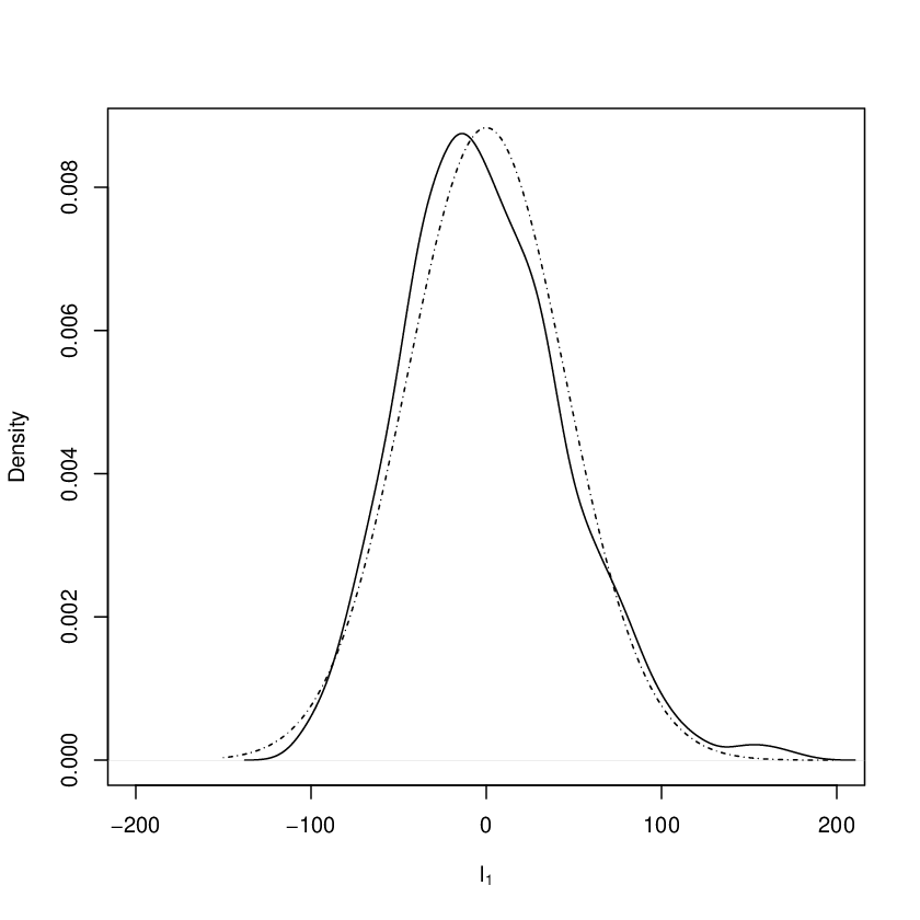
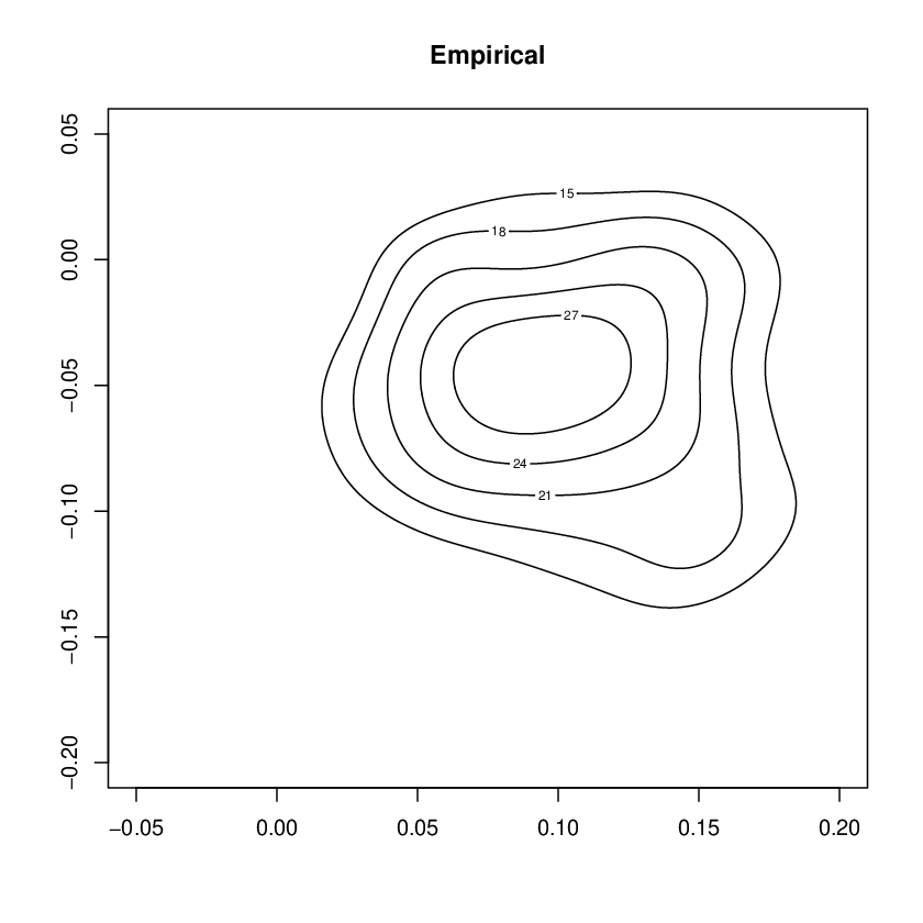
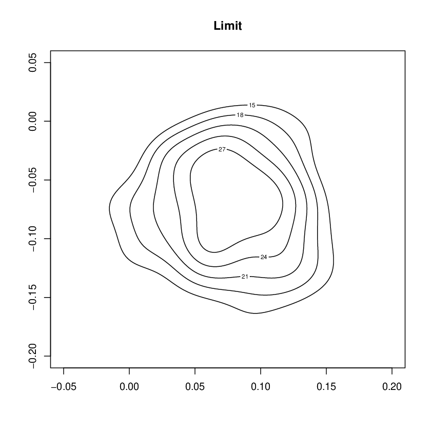
Figure 2: Upper panels show the empirical densities of l1l_{1} and lpl_{p} (solid lines, after centralisation and scaling) compared to their Gaussian limits (dashed lines). Lower panels show contour plots of empirical joint density function of (lp−2,lp−1)(l_{p-2},l_{p-1}) (left plot, after centralisation and scaling) and contour plots of their limits (right plot). Both the empirical and limit joint density functions are displayed using the two-dimensional kernel density estimates. Samples are from i.i.d. standard Gaussian distribution with U=I4U=I_{4} with 1000 independent replications.

First, we assume all the zi​jz_{ij} and wi​jw_{ij} are i.i.d. standard Gaussian, thus v4−3=0v_{4}-3=0. And according to (• ‣ 5.1), Rm​n/0.04R_{mn}/\sqrt{0.04} is the standard 2×22\times 2 Gaussian Wigner matrix (GOE). Therefore, we have

  • •

    p​{l1−42.67}→N⁡(0,4246.8)\sqrt{p}\{l_{1}-42.67\}\rightarrow N(0,4246.8) ,

  • •

    p​{lp−0.07}→N⁡(0,7.2×10−3)\sqrt{p}\{l_{p}-0.07\}\rightarrow N(0,7.2\times 10^{-3}) ,

  • •

    The two-dimensional random vector p​{lp−2−0.13,lp−1−0.13}\sqrt{p}\{l_{p-2}-0.13,l_{p-1}-0.13\} converges to the eigenvalues of the random matrix −0.138⋅W-0.138\cdot W, here WW is a 2×22\times 2 GOE.

Figure 2, upper panels, show the empirical kernel density estimates (in solid lines) of p​{l1−42.67}\sqrt{p}\{l_{1}-42.67\} and p​{lp−0.07}\sqrt{p}\{l_{p}-0.07\} from 1000 independent replications, compared to their Gaussian limits N⁡(0,4246.8)N(0,4246.8) and N⁡(0,7.2×10−3)N(0,7.2\times 10^{-3}), respectively (dashed lines). When considering the empirical distribution of the two-dimensional random vector p​{lp−2−0.13,lp−1−0.13}\sqrt{p}\{l_{p-2}-0.13,l_{p-1}-0.13\}, we run the two-dimensional kernel density estimation from 1000 independent replications and display their contour lines, see the lower-left panel of the figure, while the lower-right panel plot shows the contour lines of the kernel density estimation of the eigenvalues of the 2×22\times 2 random matrix −0.138⋅GOE-0.138\cdot GOE (their limits).

5.1.2 Binary case

Refer to caption
Refer to caption

Refer to caption Refer to caption

Figure 3: Upper panels show the empirical densities of l1l_{1} and lpl_{p} (solid lines, after centralisation and scaling) compared to their Gaussian limits (dashed lines). Lower panels show contour plots of empirical joint density function of (lp−2,lp−1)(l_{p-2},l_{p-1}) (left plot, after centralisation and scaling) and contour plots of their limits (right plot). Both the empirical and limit joint density functions are displayed using the two-dimensional kernel density estimates. Samples are from i.i.d. binary distribution with U=I4U=I_{4} and 1000 independent replications.

Second, we assume all the zi​jz_{ij} and wi​jw_{ij} are i.i.d. binary variables taking values {1,−1}\{1,-1\} with probability 1/21/2, and in this case we have v4=1v_{4}=1. Similarly, we have

  • •

    p​{l1−42.67}→N⁡(0,2039.8)\sqrt{p}\{l_{1}-42.67\}\rightarrow N(0,2039.8) ,

  • •

    p​{lp−0.07}→N⁡(0,9×10⁻⁴)\sqrt{p}\{l_{p}-0.07\}\rightarrow N(0,9\times 10^{-4}) ,

  • •

    The two-dimensional random vector p​{lp−2−0.13,lp−1−0.13}\sqrt{p}\{l_{p-2}-0.13,l_{p-1}-0.13\} converges to the eigenvalues of the random matrix −Rm​n/1.45-R_{mn}/1.45. Here, Rm​nR_{mn} is the 2×22\times 2 symmetric random matrix, made with independent Gaussian entries of mean zero and variance

    𝕍​ar​(Rm​n)={0.008,m=n,0.02,m≠n.\displaystyle\mathbb{V\text{ar}}(R_{mn})=\left\{\begin{array}[]{ll}0.008\penalty\ ,&m=n\penalty\ ,\\ 0.02\penalty\ ,&m\neq n\penalty\ .\end{array}\right.

Figure 3, upper panels, show the empirical kernel density estimates of p​{l1−42.67}\sqrt{p}\{l_{1}-42.67\} and p​{lp−0.07}\sqrt{p}\{l_{p}-0.07\} from 1000 independent replications (in solid lines), compared to their Gaussian limits (in dashed lines). Also, the lower panel on the figure show the contour lines of the empirical joint density of the p​{lp−2−0.13,lp−1−0.13}\sqrt{p}\{l_{p-2}-0.13,l_{p-1}-0.13\} (the left plot), with the right plot displaying the contour lines of their limit.

5.2 Case of general U

In this subsection, we consider the following non unit orthogonal matrix

U=(100001000012120012−12),\displaystyle U=\begin{pmatrix}1&0&0&0\\ 0&1&0&0\\ 0&0&\frac{1}{\sqrt{2}}&\frac{1}{\sqrt{2}}\\ 0&0&\frac{1}{\sqrt{2}}&\frac{-1}{\sqrt{2}}\\ \end{pmatrix}\penalty\ , (5.3)

i.e., we have

U1=(1000),U2=(0010012012),U3=(0012−12).\displaystyle U_{1}=\begin{pmatrix}1\\ 0\\ 0\\ 0\\ \end{pmatrix}\penalty\ ,\quad U_{2}=\begin{pmatrix}0&0\\ 1&0\\ 0&\frac{1}{\sqrt{2}}\\ 0&\frac{1}{\sqrt{2}}\\ \end{pmatrix}\penalty\ ,\quad U_{3}=\begin{pmatrix}0\\ 0\\ \frac{1}{\sqrt{2}}\\ \frac{-1}{\sqrt{2}}\\ \end{pmatrix}\penalty\ .

Since Gaussian distribution is invariant under orthogonal transformation, we only consider the case that all the zi​jz_{ij} and wi​jw_{ij} to be i.i.d. binary variables taking values {1,−1}\{1,-1\} with probability 1/21/2, with all the other settings fixed as in Section 5.1. Then according to Theorem 4.1, we have

  • •

    p​{l1−42.67}→N⁡(0,2039.8)\sqrt{p}\{l_{1}-42.67\}\rightarrow N(0,2039.8) ,

  • •

    p​{lp−0.07}→N⁡(0,0.004)\sqrt{p}\{l_{p}-0.07\}\rightarrow N(0,0.004) ,

  • •

    The two-dimensional random vector p​{lp−2−0.13,lp−1−0.13}\sqrt{p}\{l_{p-2}-0.13,l_{p-1}-0.13\} converges to the eigenvalues of the random matrix −U2∗R(λ2)U2/1.45-U^{*}_{2}R(\lambda_{2})U_{2}/1.45. Here, R⁡(λ2)R(\lambda_{2}) is the 4×44\times 4 symmetric random matrix, made with independent Gaussian entries of mean zero and variance

    𝕍​ar​(Rm​n)={0.008,m=n,0.02,m≠n.\displaystyle\mathbb{V\text{ar}}(R_{mn})=\left\{\begin{array}[]{ll}0.008\penalty\ ,&m=n\penalty\ ,\\ 0.02\penalty\ ,&m\neq n\penalty\ .\end{array}\right.

Figure 4, upper panels, show the empirical kernel density estimates of p​{l1−42.67}\sqrt{p}\{l_{1}-42.67\} and p​{lp−0.07}\sqrt{p}\{l_{p}-0.07\} from 1000 independent replications (in solid lines), compared to their Gaussian limits (in dashed lines). Also, the lower panel of the figure shows the contour lines of the empirical joint density of p​{lp−2−0.13,lp−1−0.13}\sqrt{p}\{l_{p-2}-0.13,l_{p-1}-0.13\} (the lower-left plot), with the lower-right plot showing the contour lines of their limit.

Refer to caption
Refer to caption

Refer to caption Refer to caption

Figure 4: Upper panels show the empirical densities of l1l_{1} and lpl_{p} (solid lines, after centralisation and scaling) compared to their Gaussian limits (dashed lines). Lower panels show contour plots of empirical joint density function of (lp−2,lp−1)(l_{p-2},l_{p-1}) (left plot, after centralisation and scaling) and contour plots of their limits (right plot). Both the empirical and limit joint density functions are displayed using the two-dimensional kernel density estimates. Samples are from i.i.d. binary distribution with UU given by (5.3) and 1000 independent replications.

6 Joint distribution of the outlier eigenvalues

In the previous section, we have obtained the following result for the outlier eigenvalues: the nin_{i}-dimensional real random vector p​{lp,j−λi,j∈Ji}\sqrt{p}\{l_{p,j}-\lambda_{i},j\in J_{i}\} converges to the distribution of the eigenvalues of random matrix −Ui∗R(λi)Ui/Δ(λi)-U^{*}_{i}R(\lambda_{i})U_{i}/\Delta(\lambda_{i}). It is in fact possible to derive their joint distribution, i.e. the limit of the MM-dimensional real random vector

(p​{lp,j1−λ1,j1∈J1}⋮p​{lp,jk−λk,jk∈Jk}).\displaystyle\left(\begin{array}[]{c}\sqrt{p}\{l_{p,j_{1}}-\lambda_{1},j_{1}\in J_{1}\}\\ \vdots\\ \sqrt{p}\{l_{p,j_{k}}-\lambda_{k},j_{k}\in J_{k}\}\end{array}\right)\penalty\ .

Such joint convergence results are useful for inference procedures where consecutive sample eigenvalues are used such as their differences or ratios, see e.g. Onatski (2009) and Passemier and Yao (2014).

Theorem 6.1.

Assume the same condition as in Theorem 4.1 and that all the population spikes aia_{i} satisfy the condition |ai−γ|>γ​c+y−c​y|a_{i}-\gamma|>\gamma\sqrt{c+y-cy}. Then the MM-dimensional vector in (6) converges in distribution to the eigenvalues of the M×MM\times M random matrix

(−U1∗​R​(λ1)​U1Δ⁡(λ1)…0⋮⋱⋮0⋯−Uk∗​R​(λk)​UkΔ⁡(λk)),\displaystyle\left(\begin{array}[]{ccc}\frac{-U^{*}_{1}R(\lambda_{1})U_{1}}{\Delta(\lambda_{1})}&\ldots&0\\ \vdots&\ddots&\vdots\\ 0&\cdots&\frac{-U^{*}_{k}R(\lambda_{k})U_{k}}{\Delta(\lambda_{k})}\end{array}\right)\penalty\ ,

where the matrices R⁡(λi)R(\lambda_{i}), made with zero-mean independent Gaussian random variables, are defined in Theorem 4.1, with the the following covariance function between different blocks (l≠sl\neq s): for 1≤i≤j≤M1\leq i\leq j\leq M,

Cov​(R⁡(λl)​(i,j),R⁡(λs)​(i,j))={θ⁡(l,s),i≠j,ω⁡(l,s)​(v4−3)+2​θ​(l,s),i=j,\displaystyle\text{Cov}(R(\lambda_{l})(i,j),R(\lambda_{s})(i,j))=\left\{\begin{array}[]{ll}\theta(l,s)\penalty\ ,&i\neq j\penalty\ ,\\ \omega(l,s)(v_{4}-3)+2\theta(l,s)\penalty\ ,&i=j\penalty\ ,\end{array}\right.

where

θ⁡(l,s)\displaystyle\theta(l,s) =lim1n+T​tr⁡An​(λl)​An​(λs),\displaystyle=\lim\frac{1}{n+T}\mathop{\text{tr}}A_{n}(\lambda_{l})A_{n}(\lambda_{s})\penalty\ ,
ω⁡(l,s)\displaystyle\omega(l,s) =lim1n+T​∑i=1n+TAn​(λl)​(i,i)​An​(λs)​(i,i),\displaystyle=\lim\frac{1}{n+T}\sum_{i=1}^{n+T}A_{n}(\lambda_{l})(i,i)A_{n}(\lambda_{s})(i,i)\penalty\ ,

and An​(λ)A_{n}(\lambda) is defined in (A).

The proof of this theorem is very close to that of Theorem 2.3 in Wang et al. (2014), thus omitted.

In principle, the limiting parameters θ⁡(l,s)\theta(l,s) and ω⁡(l,s)\omega(l,s) can be completely specified for a given spiked structure. However, this will lead to quite complex formula. Here, we prefer explain a simple case where Ωp\Omega_{p} is diagonal whose eigenvalues |ai−γ|>γ​c+y−c​y|a_{i}-\gamma|>\gamma\sqrt{c+y-cy} (i=1,⋯,Mi=1,\cdots,M) are all simple, we have U=IMU=I_{M}, M=kM=k and ni=1n_{i}=1 (i=1,⋯,Mi=1,\cdots,M). Therefore, Ui∗​R​(λi)​UiU^{*}_{i}R(\lambda_{i})U_{i} in (6.1) reduces to the (i,i)(i,i)-th element of R⁡(λi)R(\lambda_{i}), which is a Gaussian random variable. Besides, from Theorem 6.1, we see that the random variables {R⁡(λi)​(i,i)}i=1,⋯,M\{R(\lambda_{i})(i,i)\}_{i=1,\cdots,M} are jointly independent since the index sets (i,i)(i,i) are disjoint. Finally, we have the following joint distribution of the MM outlier eigenvalues of S2−1​S1S_{2}^{-1}S_{1}.

Proposition 6.1.

Under the same assumptions as in Theorem 4.1, when Ωp\Omega_{p} is diagonal with all its eigenvalues |ai−γ|>γ​c+y−c​y|a_{i}-\gamma|>\gamma\sqrt{c+y-cy} being simple, the MM outlier eigenvalues lp,jl_{p,j} (j=1,⋯,Mj=1,\cdots,M) of S2−1​S1S_{2}^{-1}S_{1} are asymptotically independent Gaussian:

(p​(lp,1−λ1)⋮p​(lp,M−λM))⟹𝒩⁡(𝟎M,(σ12⋯0⋱0⋯σM2)),\displaystyle\left(\begin{array}[]{c}\sqrt{p}(l_{p,1}-\lambda_{1})\\ \vdots\\ \sqrt{p}(l_{p,M}-\lambda_{M})\end{array}\right)\Longrightarrow\mathcal{N}\left({\bf 0}_{M},\begin{pmatrix}\sigma^{2}_{1}&\cdots&0\\ \vdots&\ddots&\vdots\\ 0&\cdots&\sigma^{2}_{M}\\ \end{pmatrix}\right)\penalty\ ,

where

σi2\displaystyle\sigma^{2}_{i} =2​ai2​(c​y−c−y)​(ai−1)2​(−1+2​ai+c+ai2​(y−1))(1+ai​(y−1))4\displaystyle=\frac{2a^{2}_{i}(cy-c-y)(a_{i}-1)^{2}(-1+2a_{i}+c+a^{2}_{i}(y-1))}{(1+a_{i}(y-1))^{4}}
+(v4−3)⋅ai2​(c+y)​(−1+2​ai+c+ai2​(y−1))2(1+ai​(y−1))4.\displaystyle\quad+(v_{4}-3)\cdot\frac{a^{2}_{i}(c+y)(-1+2a_{i}+c+a^{2}_{i}(y-1))^{2}}{(1+a_{i}(y-1))^{4}}\penalty\ .

7 Application to large-dimensional signal detection

In this section, we develop an application of the previous results to an inference problem where spiked Fisher matrices arise naturally. In a signal detection equipment, records are of form

xi=Asi+ei,i=1,…,Tx_{i}=As_{i}+e_{i}\penalty\ ,\quad i=1,\ldots,T (7.1)

where xix_{i} is pp-dimensional, sis_{i} is a k×1k\times 1 low-dimensional signal (k≪p)(k\ll p) with unit covariance matrix, AA a p×kp\times k mixing matrix, and (ei)(e_{i}) is an i.i.d. noise with covariance matrix Σ2\Sigma_{2}. Therefore, the covariance matrix of xix_{i} can be considered as a kk-dimensional perturbation of Σ2\Sigma_{2}, denoted as Σp\Sigma_{p} in the following. Notice that none of the quantities in the r.h.s. of (7.1) is observed. One of the fundamental problem here is to estimate kk, the number of signals present in the system. This problem is challenging when the dimension pp is large, say has a comparable magnitude with the sample size TT. When the noise has the simplest covariance structure, i.e. Σ2=σe2​Ip\Sigma_{2}=\sigma^{2}_{e}I_{p}, this problem has been much investigated recently and several solutions are proposed, see e.g. Kritchman and Nadler (2008), Nadler (2010), Passemier and Yao (2012); Passemier and Yao (2014). However the problem with an arbitrary noise covariance matrix Σ2\Sigma_{2}, say diagonal to simplify, remains unsolved in the large-dimensional context (to the best of our knowledge). Nevertheless, there exists an astute engineering device where the system can be tuned in a signal-free environment, for example in laboratory: that is we can directly record a sequence of pure-noise observations zjz_{j}, j=1,…,nj=1,\ldots,n, which have the same distribution as the (ei)(e_{i}) above. These signal-free records can then be used to whiten the observations (xi)(x_{i}) as follows. Let S1=T−1​∑i=1Txi​xi∗S_{1}=T^{-1}\sum_{i=1}^{T}x_{i}x_{i}^{*}, S2=n−1​∑i=1nzi​zi∗S_{2}=n^{-1}\sum_{i=1}^{n}z_{i}z_{i}^{*} and li,i=1,⋯,pl_{i},i=1,\cdots,p be the eigenvalues of S2−1​S1S_{2}^{-1}S_{1}. Notice that the eigenvalues {li}\{l_{i}\} are invariant under the transformation S1↦Σ2−1/2S1Σ2−1/2S_{1}\mapsto\Sigma_{2}^{-1/2}S_{1}\Sigma_{2}^{-1/2}, S2↦Σ2−1/2S2Σ2−1/2S_{2}\mapsto\Sigma_{2}^{-1/2}S_{2}\Sigma_{2}^{-1/2}; they are in fact independent of Σ2\Sigma_{2}. Therefore, these eigenvalues can be thought as if Σ2=Ip\Sigma_{2}=I_{p}, that is S2−1​S1S_{2}^{-1}S_{1} becomes a spiked Fisher matrix as introduced in Section 2. This is actually the reason why the two sample procedure developed here can deal with an arbitrary covariance matrix of the noise while the existing one-sample procedures cannot. Based on Theorem 3.1, we propose our estimator of the number of signals as the number of eigenvalues of S2−1​S1S_{2}^{-1}S_{1} larger than the right edge point of the support of its LSD:

k^=max⁡{i:li≥b+dn},\displaystyle\hat{k}=\max\{i:l_{i}\geq b+d_{n}\}\penalty\ , (7.2)

where (dn)(d_{n}) is a sequence of vanishing constants.

Theorem 7.1.

Assume all the spike eigenvalues aia_{i} (i=1,⋯,ki=1,\cdots,k) satisfy ai>γ+γ​c+y−c​ya_{i}>\gamma+\gamma\sqrt{c+y-cy}. Let dnd_{n} be a sequence of positive numbers such that dn→0d_{n}\rightarrow 0, p⋅dn→0\sqrt{p}\cdot d_{n}\rightarrow 0 and p2/3⋅dn→+∞p^{2/3}\cdot d_{n}\rightarrow+\infty as p→+∞p\rightarrow+\infty, then the estimator k^\hat{k} is constant, i.e. k^→k\hat{k}\rightarrow k in probability as p→+∞p\rightarrow+\infty.

Remark 7.1.

Notice here that there’s no need for those spikes aia_{i} to be simple, the only requirement is that they should be properly strong enough (ai>γ+γ​c+y−c​y)(a_{i}>\gamma+\gamma\sqrt{c+y-cy}) for detection.

Proof.

(of Theorem 7.1). Since

{k^=k}={k=max{i:li≥b+dn}}={∀j∈{1,⋯,k},lj≥b+dn}⋂{lk+1<b+dn},\displaystyle\{\hat{k}=k\}=\big\{k=\max\{i:l_{i}\geq b+d_{n}\}\big\}=\big\{\forall j\in\{1,\cdots,k\},l_{j}\geq b+d_{n}\big\}\bigcap\big\{l_{k+1}<b+d_{n}\big\}\penalty\ ,

we have

P{k^=k}\displaystyle P\{\hat{k}=k\} =P(⋂1≤j≤k{lj≥b+dn}⋂{lk+1<b+dn})\displaystyle=P\left(\bigcap_{1\leq j\leq k}\{l_{j}\geq b+d_{n}\big\}\bigcap\big\{l_{k+1}<b+d_{n}\big\}\right)
=1−P(⋃1≤j≤k{lj<b+dn}⋃{lk+1≥b+dn})\displaystyle=1-P\left(\bigcup_{1\leq j\leq k}\{l_{j}<b+d_{n}\big\}\bigcup\big\{l_{k+1}\geq b+d_{n}\big\}\right)
≥1−∑j=1kP⁡(lj<b+dn)−P⁡(lk+1≥b+dn).\displaystyle\geq 1-\sum_{j=1}^{k}P(l_{j}<b+d_{n})-P(l_{k+1}\geq b+d_{n})\penalty\ . (7.3)

For j=1,⋯,kj=1,\cdots,k,

P⁡(lj<b+dn)\displaystyle P(l_{j}<b+d_{n}) =P⁡(p​(lj−ϕ⁡(aj))<p​(b+dn−ϕ⁡(aj)))\displaystyle=P\Big(\sqrt{p}(l_{j}-\phi(a_{j}))<\sqrt{p}(b+d_{n}-\phi(a_{j}))\Big)
→P⁡(p​(lj−ϕ⁡(aj))<p​(b−ϕ⁡(aj))),\displaystyle\rightarrow P\Big(\sqrt{p}(l_{j}-\phi(a_{j}))<\sqrt{p}(b-\phi(a_{j}))\Big)\penalty\ , (7.4)

which is due to the assumption that p⋅dn→0\sqrt{p}\cdot d_{n}\rightarrow 0. Then the part p​(b−ϕ​(aj))\sqrt{p}(b-\phi(a_{j})) in (7.4) will tend to −∞-\infty since we have always ϕ⁡(aj)>b\phi(a_{j})>b when ai>γ+γ​c+y−c​ya_{i}>\gamma+\gamma\sqrt{c+y-cy}. On the other hand, by Theorem 4.1, p​(lj−ϕ⁡(aj))\sqrt{p}(l_{j}-\phi(a_{j})) in (7.4) has a limiting distribution; it is then bounded in probability. Therefore, we have

P⁡(lj<b+dn)→0for​j=1,⋯,k.\displaystyle P(l_{j}<b+d_{n})\rightarrow 0\penalty\ \quad\quad\text{for}\penalty\ j=1,\cdots,k\penalty\ . (7.5)

Also

P⁡(lk+1≥b+dn)=P⁡(p2/3​(lk+1−b)≥p2/3⋅dn),\displaystyle P(l_{k+1}\geq b+d_{n})=P\Big(p^{2/3}(l_{k+1}-b)\geq p^{2/3}\cdot d_{n}\Big)\penalty\ ,

and the part p2/3​(lk+1−b)p^{2/3}(l_{k+1}-b) is asymptotically Tracy-Widom distributed (see Bao et al. (2015) where the Tracy-Widom distribution for the largest eigenvalue of general sample covariance matrix is derived). As p2/3⋅dnp^{2/3}\cdot d_{n} tend to infinity as assumed, we have

P⁡(lk+1≥b+dn)=0.\displaystyle P(l_{k+1}\geq b+d_{n})=0\penalty\ . (7.6)

Combine (7.3), (7.5) and (7.6), we have P{k^=k}→1P\{\hat{k}=k\}\rightarrow 1 as p→+∞p\rightarrow+\infty. The proof of Theorem 7.1 is complete. ∎

We conduct a short simulation to illustrate the performance of our estimator. We fix y=1/2y=1/2 and c=1/5c=1/5 as in Section 5, and the value of pp varies from 5050 to 250250, therefore, the critical value for aia_{i} in the model (2.4) (after whitening) is ai>γ⁡{1+c+y−c​y}=3.55a_{i}>\gamma\{1+\sqrt{c+y-cy}\}=3.55. For each given pair of (p,n,T)(p,n,T), we repeat 10001000 times. The tuning parameter dnd_{n} is chosen to be (log⁡log⁡p)/p2/3(\log\log p)/p^{2/3}.

Next, suppose k=3k=3 and AA is a p×3p\times 3 matrix of form A=(c1​v1,c2​v2)A=(\sqrt{c_{1}}v_{1},\sqrt{c_{2}}v_{2}), where c1=10c_{1}=10, c2=5c_{2}=5,

v1=(10⋯0)∗andv2=(01/21/20⋯001/2−1/20⋯0)∗.\displaystyle v_{1}=\begin{pmatrix}1&0&\cdots&0\\ \end{pmatrix}^{*}\quad\text{and}\quad v_{2}=\begin{pmatrix}0&1/\sqrt{2}&1/\sqrt{2}&0&\cdots&0\\ 0&1/\sqrt{2}&-1/\sqrt{2}&0&\cdots&0\\ \end{pmatrix}^{*}\penalty\ .

Besides, assume Cov​(si)=Ik\text{Cov}(s_{i})=I_{k}. In this setting, we have two spike eigenvalues c1=10c_{1}=10, c2=5c_{2}=5 (before whitening) with multiplicity n1=1n_{1}=1, n2=2n_{2}=2, respectively. Finally, we choose Cov​(ei)\text{Cov}(e_{i}) to be either diagonal or non-diagonal as below.

Table 1: Frequency of our estimator in Model 1.
pp 50 100 150 200 250
nn 100 200 300 400 500
TT 250 500 750 1000 1250
k^=1\hat{k}=1 0.038 0.003 0 0 0.001
k^=2\hat{k}=2 0.578 0.317 0.166 0.103 0.047
k^=3{\hat{k}=3} 0.381 0.675 0.818 0.883 0.937
k^=4\hat{k}=4 0.003 0.005 0.016 0.014 0.015
  • •

    For Model 1: set Cov​(ei)=diag⁡(1,⋯,1⏟p/2,2,⋯,2⏟p/2)\text{Cov}(e_{i})=\mathop{\text{diag}}(\underbrace{1,\cdots,1}_{p/2},\underbrace{2,\cdots,2}_{p/2}) . In this case, we have the three non-zero eigenvalues of (c1​v1​v1∗+c2​v2​v2∗)⋅[Cov​(ei)]−1(c_{1}v_{1}v^{*}_{1}+c_{2}v_{2}v^{*}_{2})\cdot[\text{Cov}(e_{i})]^{-1} equal 10,5,510,5,5, respectively, which are all larger than the critical value 3.55−13.55-1, therefore, the number of detectable signals is three;

  • •

    For Model 2: set Cov​(ei)\text{Cov}(e_{i}) be compound symmetric with all the diagonal elements equal 11 and all the off-diagonal elements equal 0.10.1. In this case, we have for each given pp, the three non-zero eigenvalues of (c1​v1​v1∗+c2​v2​v2∗)⋅[Cov​(ei)]−1(c_{1}v_{1}v^{*}_{1}+c_{2}v_{2}v^{*}_{2})\cdot[\text{Cov}(e_{i})]^{-1} are all larger than 5.36(>3.55−1)5.36(>3.55-1). The number of detectable signals is again three.

Table 2: Frequency of our estimator in Model 2.
pp 50 100 150 200 250
nn 100 200 300 400 500
TT 250 500 750 1000 1250
k^=1\hat{k}=1 0.016 0 0 0 0
k^=2\hat{k}=2 0.475 0.186 0.053 0.028 0.008
k^=3{\hat{k}}=3 0.505 0.806 0.926 0.950 0.971
k^=4\hat{k}=4 0.004 0.008 0.021 0.022 0.021

Tables 1 and 2 report the empirical frequency of our estimator k^=1,2,3,4\hat{k}=1,2,3,4 in Model 1 and Model 2, respectively, where the true number of signals is k=3k=3. Also, Figure 5 shows more clearly the trends of the frequency of correct estimation in both cases. We can see the frequency both increase as pp gets larger, which confirms the consistency of our estimator.

Refer to caption Refer to caption

Figure 5: Frequency of true estimation k^=k=3\hat{k}=k=3.

References

  • Bai (2005) Bai, Z. (2005). High dimensional data analysis. Cosmos, 1(1), 17–27.
  • Bai and Ding (2012) Bai, Z. and Ding, X. (2012). Estimation of spiked eigenvalues in spiked models. Random Matrices Theory Appl., 1(2), 1150011, 21.
  • Bai and Yao (2008) Bai, Z. and Yao, J. (2008). Central limit theorems for eigenvalues in a spiked population model. Ann. Inst. Henri Poincaré Probab. Stat., 44(3), 447–474.
  • Bai and Yao (2012) Bai, Z. and Yao, J. (2012). On sample eigenvalues in a generalized spiked population model. J. Multivariate. Anal., 106, 167–177.
  • Bai et al. (1987) Bai, Z., Yin, Y.Q. and Krishnaiah P.R., (1987). On the limiting empirical distribution function of the eigenvalues of a multivariate FF-matrix. Probab. Theo. Appli. 32, 490–500.
  • Baik et al. (2005) Baik, J., Ben Arous, G., and Péché, S. 2005. Phase transition of the largest eigenvalue for nonnull complex sample covariance matrices. Ann. Probab., 33(5), 1643–1697.
  • Baik and Silverstein (2006) Baik, J. and Silverstein, J.W. (2006). Eigenvalues of Large Sample Covariance Matrices of Spiked Population Models. J. Multivariate. Anal., 97, 1382–1408.
  • Bao et al. (2015) Bao, Z. G., Pan, G.M. and Zhou, W. 2014. Universality for the largest eigenvalue of sample covariance matrices with general population. Ann. Statistics, 43(1), 382–421.
  • Benaych-Georges et al. (2011) Benaych-Georges, F., Guionnet, A. and Maïda, M. (2011). Fluctuations of the extreme eigenvalues of finite rank deformations of random matrices. Electron. J. Probab. 16(60), 1621–1662.
  • Benaych-Georges and Nadakuditi (2011) Benaych-Georges, F. and Nadakuditi, R.R. (2011). The eigenvalues and eigenvectors of finite, low rank perturbations of large random matrices. Adv. Math., 227(2), 494–521.
  • Capitaine et al. (2009) Capitaine, M., Donati-Martin, C. and Féral, D. (2009). The largest eigenvalues of finite rank deformation of large Wigner matrices: convergence and nonuniversality of the fluctuations. Ann. Probab., 37(1), 1–47.
  • Dharmawansa et al. (2014) Dharmawansa, P., Johnstone, I.M. and Onatski, A. (2014). Local asymptotic normality of the spectrum of high-dimensional spiked F-ratios. Preprint, available at arXiv:1411.3875.
  • Féral and Péché (2007) Féral, D. and Péché, S. (2007). The largest eigenvalue of rank one deformation of large Wigner matrices. Comm. Math. Phys., 272(1), 185–228.
  • Hu and Bai (2014) Hu, J. and Bai, Z.D. (2014). Strong representation of weak convergence. Science China (Mathematics) 57(11), 2399-2406.
  • Johnstone (2001) Johnstone, I. (2001). On the distribution of the largest eigenvalue in principal components analysis. Ann. Statistics, 29(2), 295–327.
  • Johnstone (2007) Johnstone, I. (2007). High dimensional statistical inference and random matrices. Pages 307–333 of: International Congress of Mathematicians. Vol. I. Eur. Math. Soc., Zürich.
  • Johnstone and Titterington (2009) Johnstone, I. and Titterington, D. (2009). Statistical challenges of high-dimensional data. Philos. Trans. R. Soc. Lond. Ser. A Math. Phys. Eng. Sci., 367(1906), 4237–4253.
  • Kritchman and Nadler (2008) Kritchman, S. and Nadler, B. (2008). Determining the number of components in a factor model from limited noisy data. Chem. Int. Lab. Syst., 94, 19–32.
  • Nadler (2010) Nadler, B. (2010). Nonparametric detection of signals by information theoretic criteria: performance analysis and an improved estimator. IEEE Trans. Signal Process., 58(5), 2746–2756.
  • Onatski (2009) Onatski, A. (2009). Testing hypotheses about the numbers of factors in large factor models. Econometrica 77, 1447–1479.
  • Passemier and Yao (2012) Passemier, D. and Yao, J. (2012). On determining the number of spikes in a high-dimensional spiked population model. Random Matrix: Theory and Applciations, doi, 10.1142/S201032631150002X.
  • Passemier and Yao (2014) Passemier, D. and Yao, J. 2014. On the detection of the number of spikes, possibly equal, in the high-dimensional case. J. Multivariate Analysis, 127, 173–183.
  • Paul (2007) Paul, D. (2007). Asymptotics of sample eigenstruture for a large dimensional spiked covariance mode. Statistica Sinica, 17, 1617–1642.
  • Paul and Aue (2014) Paul, D. and Aue, A. (2014). Random matrix theory in statistics: A review. J. Statist. Planning and Inference 150, 1-29.
  • Péché (2006) Péché, S. (2006). The largest eigenvalue of small rank perturbations of Hermitian random matrices. Probab. Theory Related Fields, 134(1), 127–173.
  • Pizzo et al. (2013) Pizzo, A., Renfrew, D. and Soshnikov, A. (2013). On finite rank deformations of Wigner matrices. Ann. Inst. Henri Poincaré Probab. Stat., 49(1), 64–94.
  • Renfrew and Soshnikov (2013) Renfrew, D., and Soshnikov, A. (2013). On finite rank deformations of Wigner matrices II: Delocalized perturbations. Random Matrices Theory Appl., 2(1), 1250015, 36.
  • Silverstein (1985) Silverstein, J. W. (1985). The limiting eigenvalue distribution of a multivariate FF matrix. SIAM J. Math. Anal. 16 (3), 641–646.
  • Skorokhod (1956) Skorokhod A. V. (1956). Limit theorems for stochastic processes. Theory Probab. Appli. 1, 261-290.
  • Wachter (1980) Wachter K. W. (1980). The limiting empirical measure of multiple discriminant ratios. Ann. Statist. 8(5), 937-957.
  • Wang et al. (2014) Wang, Q.W., Su, Z.G. and Yao, J.F. (2014). Joint CLT for several random sesquilinear forms with applications to large-dimensional spiked population models. Electron. J. Probab. 19(103), 1–28.
  • Zheng (2012) Zheng, S.R. (2012). Central Limit Theorem for Linear Spectral Statistics of Large Dimensional FF Matrix. journal=Ann. Institut Henri Poincaré Probab. Statist. 48, 444-476.
  • Zheng et al. (2013) Zheng, S.R., Bai, Z.D. and Yao, J.F. (2013). CLT for linear spectral statistics of random matrix S−1​TS^{-1}T. Preprint, available at arXiv:1305.1376.

A Some lemmas

Lemma A.1.

Let R be a M×MM\times M real-valued matrix, U=(U1⋯Uk)U=\begin{pmatrix}U_{1}&\cdots&U_{k}\\ \end{pmatrix} and V=(V1⋯Vk)V=\begin{pmatrix}V_{1}&\cdots&V_{k}\\ \end{pmatrix} are two orthogonal bases of some subspace E⊆ℝME\subseteq\mathbb{R}^{M} of dimension MM, where both UiU_{i} and ViV_{i} are of size M×niM\times n_{i}, satisfying n1+⋯nk=Mn_{1}+\cdots n_{k}=M. Then the two ni×nin_{i}\times n_{i} matrices Ui∗​R​UiU^{*}_{i}RU_{i} and Vi∗​R​ViV^{*}_{i}RV_{i} have the same eigenvalues.

Proof.

(of Lemma A.1) It is sufficient to prove that there exists a ni×nin_{i}\times n_{i} orthogonal matrix AA, such that Vi=Ui⋅AV_{i}=U_{i}\cdot A. If it is true, then Vi∗​R​Vi=A∗​(Ui∗​R​Ui)​AV^{*}_{i}RV_{i}=A^{*}(U^{*}_{i}RU_{i})A, and since AA is orthogonal, we have the eigenvalues of Vi∗​R​ViV^{*}_{i}RV_{i} and Ui∗​R​UiU^{*}_{i}RU_{i} are the same. Now let Ui=(u1⋯uni)U_{i}=\begin{pmatrix}u_{1}&\cdots&u_{n_{i}}\\ \end{pmatrix} and Vi=(v1⋯vni).V_{i}=\begin{pmatrix}v_{1}&\cdots&v_{n_{i}}\\ \end{pmatrix}. Define A=(al​s)1≤l,s≤niA=(a_{ls})_{1\leq l,s\leq n_{i}}, such that

{v1=a11u1+⋯ani​ 1uni⋮vni=a1​niu1+⋯ani​niuni.\displaystyle\left\{\begin{array}[]{c}v_{1}=a_{11}u_{1}+\cdots a_{n_{i}\,1}u_{n_{i}}\\ \vdots\\ v_{n_{i}}=a_{1n_{i}}u_{1}+\cdots a_{n_{i}\,n_{i}}u_{n_{i}}\end{array}\right.\penalty\ .

Put in matrix form:

(v1⋯vni)=(u1⋯uni)​(a11⋯a1​ni⋱0⋯ani​ni),\displaystyle\begin{pmatrix}v_{1}&\cdots&v_{n_{i}}\\ \end{pmatrix}=\begin{pmatrix}u_{1}&\cdots&u_{n_{i}}\\ \end{pmatrix}\begin{pmatrix}a_{11}&\cdots&a_{1\,n_{i}}\\ \vdots&\ddots&\vdots\\ 0&\cdots&a_{n_{i}\,n_{i}}\\ \end{pmatrix}\penalty\ ,

i.e. Vi=Ui⋅AV_{i}=U_{i}\cdot A. Since <vi,vj>=<a⋅i,a⋅j><v_{i},v_{j}>\penalty\ =\penalty\ <a_{\cdot i},a_{\cdot j}> by orthogonality of {uj}\{u_{j}\}, where a⋅k=(al​k)1≤k≤nia_{\cdot k}=(a_{lk})_{1\leq k\leq n_{i}}, therefore, the matrix AA is orthogonal. ∎

Lemma A.2.

Suppose X=(x1,⋯,xn)X=(x_{1},\cdots,x_{n}) is a p×np\times n matrix, whose columns {xi}\{x_{i}\} are independent random vectors. Y=(y1,⋯,yn)Y=(y_{1},\cdots,y_{n}) is also similarly defined. Let Σp\Sigma_{p} be the covariance matrix of xix_{i} and yiy_{i}, AA is a deterministic matrix, then we have

X​A​Y∗⟶tr⁡A⋅Σp.\displaystyle XAY^{*}\longrightarrow\mathop{\text{tr}}A\cdot\Sigma_{p}\penalty\ .

Moreover, if A is random but independent of XX and YY, then we have

X​A​Y∗⟶𝔼​tr⁡A⋅Σp.\displaystyle XAY^{*}\longrightarrow\mathbb{E}\mathop{\text{tr}}A\cdot\Sigma_{p}\penalty\ . (A.1)
Proof.

We consider the (i,j)(i,j)-th entry of X​A​Y∗XAY^{*}:

X​A​Y∗​(i,j)=∑k,l=1nX⁡(i,k)​A​(k,l)​Y∗​(l,j)=∑k,l=1nXi​k​Yj​l​Ak​l.\displaystyle XAY^{*}(i,j)=\sum_{k,l=1}^{n}X(i,k)A(k,l)Y^{*}(l,j)=\sum_{k,l=1}^{n}X_{ik}Y_{jl}A_{kl}\penalty\ . (A.2)

Since Xi​k​Yj​l→Σp​(i,j)X_{ik}Y_{jl}\rightarrow\Sigma_{p}(i,j) when k=lk=l. Therefore, the right hand side of (A.2) tends to Σp​(i,j)⋅∑k=1nAk​k\Sigma_{p}(i,j)\cdot\sum_{k=1}^{n}A_{kk}, which is equivalent to say that

X​A​Y∗→tr⁡A⋅Σp.\displaystyle XAY^{*}\rightarrow\mathop{\text{tr}}A\cdot\Sigma_{p}\penalty\ .

Then (A.1) is simply due to the conditional expectation. The proof of Lemma A.2 is complete. ∎

In all the following, λ\lambda refers to the outlier limit that

λ=a⁡(a−1+c)a−1−a​y.\lambda=\frac{a(a-1+c)}{a-1-ay}\penalty\ .
Lemma A.3.

We have

s⁡(λ)=a⁡(y−1)+1(a−1)​(a+c−1),\displaystyle s(\lambda)=\frac{a(y-1)+1}{(a-1)(a+c-1)}\penalty\ ,
m1​(λ)=(a⁡(y−1)+1)2​(−1+2​a+a2​(y−1)+y⁡(c−1))(a−1)2​(a+c−1)2​(−1+2​a+c+a2​(y−1)),\displaystyle m_{1}(\lambda)=\frac{(a(y-1)+1)^{2}(-1+2a+a^{2}(y-1)+y(c-1))}{(a-1)^{2}(a+c-1)^{2}(-1+2a+c+a^{2}(y-1))}\penalty\ ,
m2​(λ)=1a−1,\displaystyle m_{2}(\lambda)=\frac{1}{a-1}\penalty\ ,
m3​(λ)=−(a⁡(y−1)+1)2(a−1)2​(−1+2​a+c+a2​(y−1)),\displaystyle m_{3}(\lambda)=\frac{-(a(y-1)+1)^{2}}{(a-1)^{2}(-1+2a+c+a^{2}(y-1))}\penalty\ ,
m4​(λ)=−1+2​a+c+a2​(−1+c⁡(y−1))(a−1)2​(−1+2​a+c+a2​(y−1)).\displaystyle m_{4}(\lambda)=\frac{-1+2a+c+a^{2}(-1+c(y-1))}{(a-1)^{2}(-1+2a+c+a^{2}(y-1))}\penalty\ .
Proof.

(sketch of the proof of Lemma A.3) In this short proof, we skip all the detailed calculations. Recall the definition of s¯​(z)\underline{s}(z) in (3.22), its value at λ\lambda is

s¯​(λ)=a⁡(y−1)+1(a−1)​(a+c−1).\displaystyle\underline{s}(\lambda)=\frac{a(y-1)+1}{(a-1)(a+c-1)}\penalty\ . (A.3)

Also, (3.22) says that s¯​(z)\underline{s}(z) is the solution of the following equation:

z⁡(c+z​y)​s¯2​(z)+(c⁡(z⁡(1−y)+1−c)+2​z​y)​s¯​(z)+c+y−c​y=0.\displaystyle z(c+zy)\underline{s}^{2}(z)+(c(z(1-y)+1-c)+2zy)\underline{s}(z)+c+y-cy=0\penalty\ . (A.4)

Taking derivatives on both sides of (A.4) and combing with (A.3) will give the value of s¯′​(λ)\underline{s}^{\prime}(\lambda). On the other hand, since it holds

s¯​(z)+1z​(1−c)=c​s​(z),\displaystyle\underline{s}(z)+\frac{1}{z}(1-c)=cs(z)\penalty\ , (A.5)

see (3.21), taking derivatives on both sides again will give the value of s′​(λ)s^{\prime}(\lambda). Finally, the above five values is just a combination of s⁡(λ)s(\lambda) and s′​(λ)s^{\prime}(\lambda).

The proof of Lemma A.3 is complete. ∎

Lemma A.4.

Under assumptions (a)-(d),

1p​tr⁡{(λ⋅1n​Z2​Z2∗−1T​X2​X2∗)−1}​⟶a.s.​1a+c−1.\frac{1}{p}\mathop{\text{tr}}\left\{\Big(\lambda\cdot\frac{1}{n}Z_{2}Z^{*}_{2}-\frac{1}{T}X_{2}X^{*}_{2}\Big)^{-1}\right\}\overset{a.s.}{\longrightarrow}\frac{1}{a+c-1}\penalty\ .
Proof.

(of Lemma A.4) We first fix 1n​Z2​Z2∗\frac{1}{n}Z_{2}Z^{*}_{2}, then we can use the result in Zheng et al. (2013) (Lemma 4.3), which says that

1p​tr⁡(1z⋅1n​Z2​Z2∗−1T​X2​X2∗)−1→m~​(z),a.s.\displaystyle\frac{1}{p}\mathop{\text{tr}}\left(\frac{1}{z}\cdot\frac{1}{n}Z_{2}Z^{*}_{2}-\frac{1}{T}X_{2}X^{*}_{2}\right)^{-1}\rightarrow\tilde{m}(z),\quad a.s.

where m~​(z)\tilde{m}(z) is the unique solution to the equation

m~​(z)=∫1xz−11−c​m~​(z)​d​Fy​(x)\displaystyle\tilde{m}(z)=\int\frac{1}{\frac{x}{z}-\frac{1}{1-c\tilde{m}(z)}}dF_{y}(x) (A.6)

satisfying

ℑ⁡(z)⋅ℑ⁡(m~​(z))≥0,\Im(z)\cdot\Im(\tilde{m}(z))\geq 0\penalty\ ,

here, Fy​(x)F_{y}(x) is the LSD of 1n​Z2​Z2∗\frac{1}{n}Z_{2}Z^{*}_{2} (deterministic), which is the standard M-P law with parameter yy. Besides, if we denote its Stieltjes transform as s⁡(z):=∫1x−z​d​Fy​(x)s(z):=\int\frac{1}{x-z}dF_{y}(x), then (A.6) could be written as

m~​(z)=∫zx−z1−c​m~​(z)​d​Fy​(x)=z⋅s⁡(z1−c​m~​(z)).\displaystyle\tilde{m}(z)=\int\frac{z}{x-\frac{z}{1-c\tilde{m}(z)}}dF_{y}(x)=z\cdot s\left(\frac{z}{1-c\tilde{m}(z)}\right)\penalty\ . (A.7)

Since we know that the Stieltjes transform of the LSD of a standard sample covariance matrix satisfies:

s⁡(z)=11−y−y​z​s​(z)−z,\displaystyle s(z)=\frac{1}{1-y-yzs(z)-z}\penalty\ , (A.8)

then we bring (A.7) into (A.8) leads to

m~​(z)z=11−y−y⋅z1−c​m~​(z)⋅m~​(z)z−z1−c​m~​(z),\displaystyle\frac{\tilde{m}(z)}{z}=\frac{1}{1-y-y\cdot\frac{z}{1-c\tilde{m}(z)}\cdot\frac{\tilde{m}(z)}{z}-\frac{z}{1-c\tilde{m}(z)}}\penalty\ ,

whose nonnegative solution is unique, which is

m~​(z)=−1+y+z−z​c+(1−y−z+z​c)2+4​z​(y​c−y−c)2​(y​c−y−c).\displaystyle\tilde{m}(z)=\frac{-1+y+z-zc+\sqrt{(1-y-z+zc)^{2}+4z(yc-y-c)}}{2(yc-y-c)}\penalty\ . (A.9)

Therefore, we have for fixed 1n​Z2​Z2∗\frac{1}{n}Z_{2}Z^{*}_{2},

1p​tr⁡(λ⋅1n​Z2​Z2∗−1T​X2​X2∗)−1→m~​(1λ)=1a+c−1\displaystyle\frac{1}{p}\mathop{\text{tr}}\Big(\lambda\cdot\frac{1}{n}Z_{2}Z^{*}_{2}-\frac{1}{T}X_{2}X^{*}_{2}\Big)^{-1}\rightarrow\tilde{m}\left(\frac{1}{\lambda}\right)=\frac{1}{a+c-1}\penalty\

almost surely. Finally, due to the fact that for each ω\omega, the ESD of 1n​Z2​Z2∗​(ω)\frac{1}{n}Z_{2}Z^{*}_{2}(\omega) will tend to the same limit (standard M-P distribution), which is independent of the choice of ω\omega. Therefore, we have for all 1n​Z2​Z2∗\frac{1}{n}Z_{2}Z^{*}_{2} (not necessarily deterministic but independent of 1T​X2​X2∗\frac{1}{T}X_{2}X^{*}_{2}),

1p​tr⁡(λ⋅1n​Z2​Z2∗−1T​X2​X2∗)−1→1a+c−1\displaystyle\frac{1}{p}\mathop{\text{tr}}\Big(\lambda\cdot\frac{1}{n}Z_{2}Z^{*}_{2}-\frac{1}{T}X_{2}X^{*}_{2}\Big)^{-1}\rightarrow\frac{1}{a+c-1}\penalty\

almost surely.

The proof of Lemma A.4 is complete. ∎

Lemma A.5.

A⁡(λ)A(\lambda), B⁡(λ)B(\lambda), C⁡(λ)C(\lambda) and D⁡(λ)D(\lambda) are defined in (4.6), then

(l−λ)⋅1n​Z1​A​(l)​Z1∗→(l−λ)⋅(1+y​λ​s​(λ))⋅IM,\displaystyle(l-\lambda)\cdot\frac{1}{n}Z_{1}A(l)Z^{*}_{1}\rightarrow(l-\lambda)\cdot(1+y\lambda s(\lambda))\cdot I_{M}\penalty\ , (A.10)
λn​Z1​[A⁡(l)−A⁡(λ)]​Z1∗→(l−λ)⋅(λ​y​s​(λ)+λ2​y​m1​(λ))⋅IM,\displaystyle\frac{\lambda}{n}Z_{1}[A(l)-A(\lambda)]Z^{*}_{1}\rightarrow(l-\lambda)\cdot(\lambda ys(\lambda)+\lambda^{2}ym_{1}(\lambda))\cdot I_{M}\penalty\ , (A.11)
1TX1(B(l)−B(λ))X1∗→−(l−λ)⋅cm3(λ)⋅U(a1⋱ak)U∗,\displaystyle\frac{1}{T}X_{1}(B(l)-B(\lambda))X^{*}_{1}\rightarrow-(l-\lambda)\cdot cm_{3}(\lambda)\cdot U\left(\begin{array}[]{c}a_{1}\\ \quad\ddots\\ \quad\quad a_{k}\end{array}\right)U^{*}\penalty\ ,
ln​Z1​(C⁡(l)−C⁡(λ))​X1∗+l−λn​Z1​C​(λ)​X1∗→(l−λ)⋅𝟎M×M,\displaystyle\frac{l}{n}Z_{1}(C(l)-C(\lambda))X^{*}_{1}+\frac{l-\lambda}{n}Z_{1}C(\lambda)X^{*}_{1}\rightarrow(l-\lambda)\cdot{\bf 0}_{M\times M}\penalty\ , (A.15)
lT​X1​(D⁡(l)−D⁡(λ))​Z1∗+l−λT​X1​D​(λ)​Z1∗→(l−λ)⋅𝟎M×M.\displaystyle\frac{l}{T}X_{1}(D(l)-D(\lambda))Z^{*}_{1}+\frac{l-\lambda}{T}X_{1}D(\lambda)Z^{*}_{1}\rightarrow(l-\lambda)\cdot{\bf 0}_{M\times M}\penalty\ . (A.16)
Proof.

(of Lemma A.5)

Proof of (A.10): Since Z1Z_{1} is independent of AA and Cov​(Z1)=IM\text{Cov}(Z_{1})=I_{M}, we combine this fact with Lemma A.2:

(l−λ)⋅1nZ1A(l)Z1∗→(l−λ)⋅1n𝔼trA(l)⋅IM.\displaystyle(l-\lambda)\cdot\frac{1}{n}Z_{1}A(l)Z^{*}_{1}\rightarrow(l-\lambda)\cdot\frac{1}{n}\mathbb{E}\mathop{\text{tr}}A(l)\cdot I_{M}\penalty\ . (A.17)

Considering the expression of A⁡(l)A(l), we have

1n​𝔼​tr⁡A⁡(λ)\displaystyle\frac{1}{n}\mathbb{E}\mathop{\text{tr}}A(\lambda) =1n​𝔼​tr⁡[In−Z2∗​(λ​Ip−S)−1​(1n​Z2​Z2∗)−1​λn​Z2]\displaystyle=\frac{1}{n}\mathbb{E}\mathop{\text{tr}}\left[I_{n}-Z^{*}_{2}(\lambda I_{p}-S)^{-1}\Big(\frac{1}{n}Z_{2}Z^{*}_{2}\Big)^{-1}\frac{\lambda}{n}Z_{2}\right]
=1−λn​𝔼​tr⁡(λ​Ip−S)−1\displaystyle=1-\frac{\lambda}{n}\mathbb{E}\mathop{\text{tr}}(\lambda I_{p}-S)^{-1}
=1−y​λ​∫1λ−x​d​Fc,y​(x)\displaystyle=1-y\lambda\int\frac{1}{\lambda-x}dF_{c,y}(x)
=1+y​λ​s​(λ).\displaystyle=1+y\lambda s(\lambda)\penalty\ .

Therefore, combine with (A.17), we have

(l−λ)⋅1n​Z1​A​(l)​Z1∗→(l−λ)​(1+y​λ​s​(λ))⋅IM.\displaystyle(l-\lambda)\cdot\frac{1}{n}Z_{1}A(l)Z^{*}_{1}\rightarrow(l-\lambda)(1+y\lambda s(\lambda))\cdot I_{M}\penalty\ .

Proof of (A.11): Bringing the expression of A⁡(l)A(l) into consideration, we first have

A⁡(l)−A⁡(λ)\displaystyle\quad A(l)-A(\lambda)
=Z2∗​(λ​Ip−S)−1​(1n​Z2​Z2∗)−1​λn​Z2−Z2∗​(l​Ip−S)−1​(1n​Z2​Z2∗)−1​ln​Z2\displaystyle=Z^{*}_{2}(\lambda I_{p}-S)^{-1}\Big(\frac{1}{n}Z_{2}Z^{*}_{2}\Big)^{-1}\frac{\lambda}{n}Z_{2}-Z^{*}_{2}(lI_{p}-S)^{-1}\Big(\frac{1}{n}Z_{2}Z^{*}_{2}\Big)^{-1}\frac{l}{n}Z_{2}
=Z2∗​(λ​Ip−S)−1​(1n​Z2​Z2∗)−1​λ−ln​Z2+Z2∗​[(λ​Ip−S)−1−(l​Ip−S)−1]​(1n​Z2​Z2∗)−1​ln​Z2\displaystyle=Z^{*}_{2}(\lambda I_{p}-S)^{-1}\Big(\frac{1}{n}Z_{2}Z^{*}_{2}\Big)^{-1}\frac{\lambda-l}{n}Z_{2}+Z^{*}_{2}\left[(\lambda I_{p}-S)^{-1}-(lI_{p}-S)^{-1}\right]\Big(\frac{1}{n}Z_{2}Z^{*}_{2}\Big)^{-1}\frac{l}{n}Z_{2}
=(l−λ)⋅[−Z2∗​(λ​Ip−S)−1​(1n​Z2​Z2∗)−1​1n​Z2+Z2∗​(λ​Ip−S)−1​(l​Ip−S)−1​(1n​Z2​Z2∗)−1​ln​Z2].\displaystyle=(l-\lambda)\cdot\left[-Z^{*}_{2}(\lambda I_{p}-S)^{-1}\Big(\frac{1}{n}Z_{2}Z^{*}_{2}\Big)^{-1}\frac{1}{n}Z_{2}+Z^{*}_{2}(\lambda I_{p}-S)^{-1}(lI_{p}-S)^{-1}\Big(\frac{1}{n}Z_{2}Z^{*}_{2}\Big)^{-1}\frac{l}{n}Z_{2}\right]\penalty\ .

Then using Lemma A.2 for the same reason, we have

λn​Z1​[A⁡(l)−A⁡(λ)]​Z1∗→λn​{𝔼​tr⁡(A⁡(l)−A⁡(λ))}⋅IM,\displaystyle\quad\frac{\lambda}{n}Z_{1}[A(l)-A(\lambda)]Z^{*}_{1}\rightarrow\frac{\lambda}{n}\left\{\mathbb{E}\mathop{\text{tr}}\left(A(l)-A(\lambda)\right)\right\}\cdot I_{M}\penalty\ ,

and

1n𝔼tr(A(l)−A(λ))=(l−λ)⋅[−1n𝔼tr{Z2∗(λIp−S)−1(1nZ2Z2∗)−11nZ2}\displaystyle\quad\frac{1}{n}\mathbb{E}\mathop{\text{tr}}\left(A(l)-A(\lambda)\right)=(l-\lambda)\cdot\bigg[-\frac{1}{n}\mathbb{E}\mathop{\text{tr}}\left\{Z^{*}_{2}(\lambda I_{p}-S)^{-1}\Big(\frac{1}{n}Z_{2}Z^{*}_{2}\Big)^{-1}\frac{1}{n}Z_{2}\right\}
+1n𝔼tr{Z2∗(λIp−S)−1(lIp−S)−1(1nZ2Z2∗)−1lnZ2}]\displaystyle\quad\quad\quad\quad\quad\quad\quad\quad+\frac{1}{n}\mathbb{E}\mathop{\text{tr}}\left\{Z^{*}_{2}(\lambda I_{p}-S)^{-1}(lI_{p}-S)^{-1}\Big(\frac{1}{n}Z_{2}Z^{*}_{2}\Big)^{-1}\frac{l}{n}Z_{2}\right\}\bigg]
=(l−λ)⋅[−1n𝔼tr(λIp−S)−1+λn𝔼tr(λIp−S)−2+o(1)]\displaystyle=(l-\lambda)\cdot\bigg[-\frac{1}{n}\mathbb{E}\mathop{\text{tr}}(\lambda I_{p}-S)^{-1}+\frac{\lambda}{n}\mathbb{E}\mathop{\text{tr}}(\lambda I_{p}-S)^{-2}+o(1)\bigg]
=(l−λ)⋅[y​∫1x−λ​d​Fc,y​(x)+λ​y​∫1(λ−x)2​d​Fc,y​(x)+o⁡(1)]\displaystyle=(l-\lambda)\cdot\Big[y\int\frac{1}{x-\lambda}dF_{c,y}(x)+\lambda y\int\frac{1}{(\lambda-x)^{2}}dF_{c,y}(x)+o(1)\Big]
=(l−λ)⋅[y​s​(λ)+λ​y​m1​(λ)+o⁡(1)].\displaystyle=(l-\lambda)\cdot\Big[ys(\lambda)+\lambda ym_{1}(\lambda)+o(1)\Big]\penalty\ .

Therefore, we have

λn​Z1​[A⁡(l)−A⁡(λ)]​Z1∗→(l−λ)⋅(y​λ​s​(λ)+λ2​y​m1​(λ))⋅IM.\displaystyle\quad\frac{\lambda}{n}Z_{1}[A(l)-A(\lambda)]Z^{*}_{1}\rightarrow(l-\lambda)\cdot(y\lambda s(\lambda)+\lambda^{2}ym_{1}(\lambda))\cdot I_{M}\penalty\ .

Proof of (A.5):
First recall the fact that Cov​(X1)=U​(a1⋱ak)​U∗\text{Cov}(X_{1})=U\left(\begin{array}[]{c}a_{1}\\ \quad\ddots\\ \quad\quad a_{k}\end{array}\right)U^{*}\penalty\ and X1X_{1} is independent of BB. Using Lemma A.2,we have

1T​X1​(B⁡(l)−B⁡(λ))​X1∗→1T​𝔼​tr⁡(B⁡(l)−B⁡(λ))⋅U​(a1⋱ak)​U∗.\displaystyle\frac{1}{T}X_{1}(B(l)-B(\lambda))X^{*}_{1}\rightarrow\frac{1}{T}\mathbb{E}\mathop{\text{tr}}(B(l)-B(\lambda))\cdot U\left(\begin{array}[]{c}a_{1}\\ \quad\ddots\\ \quad\quad a_{k}\end{array}\right)U^{*}\penalty\ .

The part

1T​𝔼​tr⁡(B⁡(l)−B⁡(λ))\displaystyle\quad\frac{1}{T}\mathbb{E}\mathop{\text{tr}}(B(l)-B(\lambda))
=1T​𝔼​tr⁡{X2∗​[(l​Ip−S)−1−(λ​Ip−S)−1]​(1n​Z2​Z2∗)−1​1T​X2}\displaystyle=\frac{1}{T}\mathbb{E}\mathop{\text{tr}}\left\{X^{*}_{2}\bigg[(lI_{p}-S)^{-1}-(\lambda I_{p}-S)^{-1}\bigg]\Big(\frac{1}{n}Z_{2}Z^{*}_{2}\Big)^{-1}\frac{1}{T}X_{2}\right\}
=(l−λ)⋅[−1T𝔼tr{(λIp−S)−2S}+o(1)]\displaystyle=(l-\lambda)\cdot\left[-\frac{1}{T}\mathbb{E}\mathop{\text{tr}}\left\{(\lambda I_{p}-S)^{-2}S\right\}+o(1)\right]
=(l−λ)⋅[−c∫x(λ−x)2dFc,y(x)+o(1)]\displaystyle=(l-\lambda)\cdot\left[-c\int\frac{x}{(\lambda-x)^{2}}dF_{c,y}(x)+o(1)\right]
=(l−λ)⋅(−c​m3​(λ)+o⁡(1)).\displaystyle=(l-\lambda)\cdot(-cm_{3}(\lambda)+o(1))\penalty\ .

Therefore, we have

1TX1(B(l)−B(λ))X1∗→−c(l−λ)m3(λ)⋅U(a1⋱ak)U∗.\displaystyle\frac{1}{T}X_{1}(B(l)-B(\lambda))X^{*}_{1}\rightarrow-c(l-\lambda)m_{3}(\lambda)\cdot U\left(\begin{array}[]{c}a_{1}\\ \quad\ddots\\ \quad\quad a_{k}\end{array}\right)U^{*}\penalty\ .

Proof of (A.15) and (A.16): (A.15) and (A.16) are derived simply due to the fact that Cov​(X1,Z1)=𝟎M×M\text{Cov}(X_{1},Z_{1})={\bf 0}_{M\times M} .

The proof of Lemma A.5 is complete. ∎

Lemma A.6.

Define

R~n​(λi):=(Z1S1)​(λi​p​A​(λi)nλi​ai​p​C​(λi)nλi​ai​p​D​(λi)T−ai​p​B​(λi)T)​(Z1∗S1∗)−𝔼⁡[⋅].\displaystyle\tilde{R}_{n}(\lambda_{i}):=\begin{pmatrix}Z_{1}&S_{1}\\ \end{pmatrix}\left(\begin{array}[]{cc}\frac{\lambda_{i}\sqrt{p}A(\lambda_{i})}{n}&\frac{\lambda_{i}\sqrt{a_{i}p}C(\lambda_{i})}{n}\\[5.69054pt] \frac{\lambda_{i}\sqrt{a_{i}p}D(\lambda_{i})}{T}&\frac{-a_{i}\sqrt{p}B(\lambda_{i})}{T}\end{array}\right)\begin{pmatrix}Z^{*}_{1}\\[8.53581pt] S^{*}_{1}\\ \end{pmatrix}-\mathbb{E}[\cdot]\penalty\ .

then R~n​(λi)\tilde{R}_{n}(\lambda_{i}) weakly converges to a M×MM\times M symmetric random matrix R⁡(λi)=(Rm​n)R(\lambda_{i})=(R_{mn}), which is made with independent Gaussian entries of mean zero and variance

𝕍​ar​(Rm​n)={2​θi+(v4−3)​ωi,m=n,θi,m≠n,\displaystyle\mathbb{V\text{ar}}(R_{mn})=\left\{\begin{array}[]{ll}2\theta_{i}+(v_{4}-3)\omega_{i}\penalty\ ,&m=n\penalty\ ,\\ \theta_{i}\penalty\ ,&m\neq n\penalty\ ,\end{array}\right.

where

ωi=ai2​(ai+c−1)2​(c+y)(ai−1)2,\displaystyle\omega_{i}=\frac{a_{i}^{2}(a_{i}+c-1)^{2}(c+y)}{(a_{i}-1)^{2}}\penalty\ ,
θi=ai2​(ai+c−1)2​(c​y−c−y)−1+2​ai+c+ai2​(y−1).\displaystyle\theta_{i}=\frac{a_{i}^{2}(a_{i}+c-1)^{2}(cy-c-y)}{-1+2a_{i}+c+a_{i}^{2}(y-1)}\penalty\ .
Proof.

Since Z1Z_{1} and S1S_{1} are independent, having the same first four moments, both are made with i.i.d. components, we can now view (Z1S1)\left(\begin{array}[]{cc}Z_{1}&S_{1}\end{array}\right) as a M×(n+T)M\times(n+T) table ξ\xi, made with i.i.d elements of mean 0 and variance 1. Besides, we can rewrite the expression of A⁡(λ)A(\lambda), B⁡(λ)B(\lambda), C⁡(λ)C(\lambda) and D⁡(λ)D(\lambda) as follows:

A⁡(λ)\displaystyle A(\lambda) =In−Z2∗​(λ⋅1n​Z2​Z2∗−1T​X2​X2∗)−1​λn​Z2,\displaystyle=I_{n}-Z^{*}_{2}\Big(\lambda\cdot\frac{1}{n}Z_{2}Z^{*}_{2}-\frac{1}{T}X_{2}X^{*}_{2}\Big)^{-1}\frac{\lambda}{n}Z_{2}\penalty\ ,
B⁡(λ)\displaystyle B(\lambda) =IT+X2∗​(λ⋅1n​Z2​Z2∗−1T​X2​X2∗)−1​1T​X2,\displaystyle=I_{T}+X^{*}_{2}\Big(\lambda\cdot\frac{1}{n}Z_{2}Z^{*}_{2}-\frac{1}{T}X_{2}X^{*}_{2}\Big)^{-1}\frac{1}{T}X_{2}\penalty\ ,
C⁡(λ)\displaystyle C(\lambda) =Z2∗​(λ⋅1n​Z2​Z2∗−1T​X2​X2∗)−1​1T​X2,\displaystyle=Z^{*}_{2}\Big(\lambda\cdot\frac{1}{n}Z_{2}Z^{*}_{2}-\frac{1}{T}X_{2}X^{*}_{2}\Big)^{-1}\frac{1}{T}X_{2}\penalty\ ,
D⁡(λ)\displaystyle D(\lambda) =X2∗​(λ⋅1n​Z2​Z2∗−1T​X2​X2∗)−1​1n​Z2.\displaystyle=X^{*}_{2}\Big(\lambda\cdot\frac{1}{n}Z_{2}Z^{*}_{2}-\frac{1}{T}X_{2}X^{*}_{2}\Big)^{-1}\frac{1}{n}Z_{2}\penalty\ .

It holds

A​(λ)∗=A⁡(λ),B​(λ)∗=B⁡(λ),T⋅C​(λ)∗=n⋅D⁡(λ),\displaystyle A(\lambda)^{*}=A(\lambda)\penalty\ ,\penalty\ B(\lambda)^{*}=B(\lambda)\penalty\ ,\penalty\ T\cdot C(\lambda)^{*}=n\cdot D(\lambda)\penalty\ ,

therefore, the matrix

(λi​p​A​(λi)nλi​ai​p​C​(λi)nλi​ai​p​D​(λi)T−ai​p​B​(λi)T)\displaystyle\left(\begin{array}[]{cc}\frac{\lambda_{i}\sqrt{p}A(\lambda_{i})}{n}&\frac{\lambda_{i}\sqrt{a_{i}p}C(\lambda_{i})}{n}\\[5.69054pt] \frac{\lambda_{i}\sqrt{a_{i}p}D(\lambda_{i})}{T}&\frac{-a_{i}\sqrt{p}B(\lambda_{i})}{T}\end{array}\right)

is symmetric. Define

An​(λi)=n+T⋅(λi​p​A​(λi)nλi​ai​p​C​(λi)nλi​ai​p​D​(λi)T−ai​p​B​(λi)T).\displaystyle A_{n}(\lambda_{i})=\sqrt{n+T}\cdot\left(\begin{array}[]{cc}\frac{\lambda_{i}\sqrt{p}A(\lambda_{i})}{n}&\frac{\lambda_{i}\sqrt{a_{i}p}C(\lambda_{i})}{n}\\[5.69054pt] \frac{\lambda_{i}\sqrt{a_{i}p}D(\lambda_{i})}{T}&\frac{-a_{i}\sqrt{p}B(\lambda_{i})}{T}\end{array}\right)\penalty\ .

Now we can apply the results in Bai and Yao (2008) (Proposition 3.1 and Remark 1), which says that R~n​(λi)\tilde{R}_{n}(\lambda_{i}) weakly converges to a M×MM\times M symmetric random matrix R⁡(λi)=(Rm​n)R(\lambda_{i})=(R_{mn}), which is made with i.i.d. Gaussian entries of mean zero and variance

𝕍​ar​(Rm​n)={2​θi+(v4−3)​ωi,m=n,θi,m≠n,\displaystyle\mathbb{V\text{ar}}(R_{mn})=\left\{\begin{array}[]{ll}2\theta_{i}+(v_{4}-3)\omega_{i}\penalty\ ,&m=n\penalty\ ,\\ \theta_{i}\penalty\ ,&m\neq n\penalty\ ,\end{array}\right.

The following is devoted to the calculation of the values of θi\theta_{i} and ωi\omega_{i}.

Calculating of θi\theta_{i}: From the definition of θ\theta (see Bai and Yao (2008) for details), we have

θi\displaystyle\theta_{i} =lim1n+T​tr⁡An2​(λi)\displaystyle=\lim\frac{1}{n+T}\mathop{\text{tr}}A^{2}_{n}(\lambda_{i})
=limtr⁡(λi​p​A​(λi)nλi​ai​p​C​(λi)nλi​ai​p​D​(λi)T−ai​p​B​(λi)T)​(λi​p​A​(λi)nλi​ai​p​C​(λi)nλi​ai​p​D​(λi)T−ai​p​B​(λi)T)\displaystyle=\lim\mathop{\text{tr}}\left(\begin{array}[]{cc}\frac{\lambda_{i}\sqrt{p}A(\lambda_{i})}{n}&\frac{\lambda_{i}\sqrt{a_{i}p}C(\lambda_{i})}{n}\\[5.69054pt] \frac{\lambda_{i}\sqrt{a_{i}p}D(\lambda_{i})}{T}&\frac{-a_{i}\sqrt{p}B(\lambda_{i})}{T}\end{array}\right)\left(\begin{array}[]{cc}\frac{\lambda_{i}\sqrt{p}A(\lambda_{i})}{n}&\frac{\lambda_{i}\sqrt{a_{i}p}C(\lambda_{i})}{n}\\[5.69054pt] \frac{\lambda_{i}\sqrt{a_{i}p}D(\lambda_{i})}{T}&\frac{-a_{i}\sqrt{p}B(\lambda_{i})}{T}\end{array}\right)
=limtr⁡(p​λi2n2​A2​(λi)+λi2​ai​pn​T​C​(λi)​D​(λi)⋆⋆λi2​ai​pn​T​D​(λi)​C​(λi)+ai2​pT2​B2​(λi))\displaystyle=\lim\mathop{\text{tr}}\left(\begin{array}[]{cc}\frac{p\lambda_{i}^{2}}{n^{2}}A^{2}(\lambda_{i})+\frac{\lambda_{i}^{2}a_{i}p}{nT}C(\lambda_{i})D(\lambda_{i})&\star\\[5.69054pt] \star&\frac{\lambda_{i}^{2}a_{i}p}{nT}D(\lambda_{i})C(\lambda_{i})+\frac{a^{2}_{i}p}{T^{2}}B^{2}(\lambda_{i})\end{array}\right)
=lim[p​λi2n2​tr⁡A2​(λi)+2​λi2​ai​pn​T​tr⁡C⁡(λi)​D​(λi)+ai2​pT2​tr⁡B2​(λi)].\displaystyle=\lim\left[\frac{p\lambda_{i}^{2}}{n^{2}}\mathop{\text{tr}}A^{2}(\lambda_{i})+\frac{2\lambda_{i}^{2}a_{i}p}{nT}\mathop{\text{tr}}C(\lambda_{i})D(\lambda_{i})+\frac{a^{2}_{i}p}{T^{2}}\mathop{\text{tr}}B^{2}(\lambda_{i})\right]\penalty\ . (A.26)
tr⁡A2​(λi)\displaystyle\mathop{\text{tr}}A^{2}(\lambda_{i}) =tr[In+Z2∗(λiIp−S)−1(1nZ2Z2∗)−1λinZ2Z2∗(λiIp−S)−1(1nZ2Z2∗)−1λinZ2\displaystyle=\mathop{\text{tr}}\left[I_{n}+Z^{*}_{2}(\lambda_{i}I_{p}-S)^{-1}\left(\frac{1}{n}Z_{2}Z^{*}_{2}\right)^{-1}\frac{\lambda_{i}}{n}Z_{2}Z^{*}_{2}(\lambda_{i}I_{p}-S)^{-1}\left(\frac{1}{n}Z_{2}Z^{*}_{2}\right)^{-1}\frac{\lambda_{i}}{n}Z_{2}\right.
−2Z2∗(λiIp−S)−1(1nZ2Z2∗)−1λinZ2]\displaystyle\quad\quad\left.-2Z^{*}_{2}(\lambda_{i}I_{p}-S)^{-1}\left(\frac{1}{n}Z_{2}Z^{*}_{2}\right)^{-1}\frac{\lambda_{i}}{n}Z_{2}\right]
=n+λi2​tr⁡(λi​Ip−S)−2−2​λi​tr⁡(λi​Ip−S)−1\displaystyle=n+\lambda_{i}^{2}\mathop{\text{tr}}(\lambda_{i}I_{p}-S)^{-2}-2\lambda_{i}\mathop{\text{tr}}(\lambda_{i}I_{p}-S)^{-1}
=n+p​λi2​m1​(λi)+2​p​λi​s​(λi),\displaystyle=n+p\lambda_{i}^{2}m_{1}(\lambda_{i})+2p\lambda_{i}s(\lambda_{i})\penalty\ , (A.27)
tr⁡C⁡(λi)​D​(λi)\displaystyle\mathop{\text{tr}}C(\lambda_{i})D(\lambda_{i}) =tr⁡{Z2∗​(λi​Ip−S)−1​(1n​Z2​Z2∗)−1​1T​X2​X2∗​(λi​Ip−S)−1​(1n​Z2​Z2∗)−1​1n​Z2}\displaystyle=\mathop{\text{tr}}\left\{Z^{*}_{2}(\lambda_{i}I_{p}-S)^{-1}\left(\frac{1}{n}Z_{2}Z^{*}_{2}\right)^{-1}\frac{1}{T}X_{2}X^{*}_{2}(\lambda_{i}I_{p}-S)^{-1}\left(\frac{1}{n}Z_{2}Z^{*}_{2}\right)^{-1}\frac{1}{n}Z_{2}\right\}
=tr⁡(λi​Ip−S)−1​S​(λi​Ip−S)−1=p​m3​(λi)\displaystyle=\mathop{\text{tr}}(\lambda_{i}I_{p}-S)^{-1}S(\lambda_{i}I_{p}-S)^{-1}=pm_{3}(\lambda_{i}) (A.28)
tr⁡B2​(λi)\displaystyle\mathop{\text{tr}}B^{2}(\lambda_{i}) =tr[IT+X2∗(λiIp−S)−1(1nZ2Z2∗)−11TX2X2∗(λiIp−S)−1(1nZ2Z2∗)−11TX2\displaystyle=\mathop{\text{tr}}\left[I_{T}+X^{*}_{2}(\lambda_{i}I_{p}-S)^{-1}\left(\frac{1}{n}Z_{2}Z^{*}_{2}\right)^{-1}\frac{1}{T}X_{2}X^{*}_{2}(\lambda_{i}I_{p}-S)^{-1}\left(\frac{1}{n}Z_{2}Z^{*}_{2}\right)^{-1}\frac{1}{T}X_{2}\right.
+2X2∗(λiIp−S)−1(1nZ2Z2∗)−11TX2]\displaystyle\quad\quad\left.+2X^{*}_{2}(\lambda_{i}I_{p}-S)^{-1}\left(\frac{1}{n}Z_{2}Z^{*}_{2}\right)^{-1}\frac{1}{T}X_{2}\right]
=T+tr⁡(λi​Ip−S)−1​F​(λi​Ip−S)−1​S+2​tr⁡(λi​Ip−S)−1​S\displaystyle=T+\mathop{\text{tr}}(\lambda_{i}I_{p}-S)^{-1}F(\lambda_{i}I_{p}-S)^{-1}S+2\mathop{\text{tr}}(\lambda_{i}I_{p}-S)^{-1}S
=T+p​m4​(λi)+2​p​m2​(λi),\displaystyle=T+pm_{4}(\lambda_{i})+2pm_{2}(\lambda_{i})\penalty\ , (A.29)

Combining (A.26), (A.27), (A.28) and (A.29), we have

θi\displaystyle\theta_{i} =λi2​y​(1+y​λi2​m1​(λi)+2​y​λi​s​(λi))+2​λi2​ai​c​y​m3​(λi)+ai2​c​(1+c​m4​(λi)+2​c​m2​(λi))\displaystyle=\lambda_{i}^{2}y(1+y\lambda_{i}^{2}m_{1}(\lambda_{i})+2y\lambda_{i}s(\lambda_{i}))+2\lambda_{i}^{2}a_{i}cym_{3}(\lambda_{i})+a^{2}_{i}c(1+cm_{4}(\lambda_{i})+2cm_{2}(\lambda_{i}))
=ai2​(ai+c−1)2​(c​y−c−y)−1+2​ai+c+ai2​(y−1).\displaystyle=\frac{a^{2}_{i}(a_{i}+c-1)^{2}(cy-c-y)}{-1+2a_{i}+c+a^{2}_{i}(y-1)}.

Calculating of ωi\omega_{i}:

ωi=lim1n+T​∑i=1n+T(An​(λi)​(i,i))2=lim[∑i=1nλi2​pn2​A2​(i,i)+∑i=1Tai2​pT2​B2​(i,i)].\displaystyle\omega_{i}=\lim\frac{1}{n+T}\sum_{i=1}^{n+T}(A_{n}(\lambda_{i})(i,i))^{2}=\lim\left[\sum_{i=1}^{n}\frac{\lambda_{i}^{2}p}{n^{2}}A^{2}(i,i)+\sum_{i=1}^{T}\frac{a^{2}_{i}p}{T^{2}}B^{2}(i,i)\right]\penalty\ . (A.30)

In the following, we will show that A⁡(i,i)A(i,i) and B⁡(i,i)B(i,i) both tend to some limits that is independent of ii.

A⁡(i,i)\displaystyle A(i,i) =1−[Z2∗​[λi​Ip−(1n​Z2​Z2∗)−1​1T​X2​X2∗]−1​(1n​Z2​Z2∗)−1​λin​Z2]​(i,i)\displaystyle=1-\bigg[Z^{*}_{2}\Big[\lambda_{i}I_{p}-\big(\frac{1}{n}Z_{2}Z^{*}_{2}\big)^{-1}\frac{1}{T}X_{2}X^{*}_{2}\Big]^{-1}\big(\frac{1}{n}Z_{2}Z^{*}_{2}\big)^{-1}\frac{\lambda_{i}}{n}Z_{2}\bigg](i,i)
=1−λin​[Z2∗​[λi⋅1n​Z2​Z2∗−1T​X2​X2∗]−1​Z2]​(i,i)\displaystyle=1-\frac{\lambda_{i}}{n}\bigg[Z^{*}_{2}\Big[\lambda_{i}\cdot\frac{1}{n}Z_{2}Z^{*}_{2}-\frac{1}{T}X_{2}X^{*}_{2}\Big]^{-1}Z_{2}\bigg](i,i) (A.31)

If we denote ηi\eta_{i} as the ii-th column of Z2Z_{2}, we have

1n​Z2​Z2∗=1n​(η1⋯ηn)⋅(η1∗ηn∗)=1n​ηi​ηi∗+1n​Z2​i​Z2​i∗,\displaystyle\frac{1}{n}Z_{2}Z^{*}_{2}=\frac{1}{n}\begin{pmatrix}\eta_{1}&\cdots&\eta_{n}\\ \end{pmatrix}\cdot\begin{pmatrix}\eta^{*}_{1}\\ \vdots\\ \eta^{*}_{n}\\ \end{pmatrix}=\frac{1}{n}\eta_{i}\eta^{*}_{i}+\frac{1}{n}Z_{2i}Z^{*}_{2i}\penalty\ ,

where Z2​iZ_{2i} is independent of ηi\eta_{i}. Since

(λi⋅1n​Z2​Z2∗−1T​X2​X2∗)−1−(λi⋅1n​Z2​i​Z2​i∗−1T​X2​X2∗)−1\displaystyle\quad\Big(\lambda_{i}\cdot\frac{1}{n}Z_{2}Z^{*}_{2}-\frac{1}{T}X_{2}X^{*}_{2}\Big)^{-1}-\Big(\lambda_{i}\cdot\frac{1}{n}Z_{2i}Z^{*}_{2i}-\frac{1}{T}X_{2}X^{*}_{2}\Big)^{-1}
=−(λi⋅1n​Z2​Z2∗−1T​X2​X2∗)−1​λin​ηi​ηi∗​(λi⋅1n​Z2​i​Z2​i∗−1T​X2​X2∗)−1,\displaystyle=-\Big(\lambda_{i}\cdot\frac{1}{n}Z_{2}Z^{*}_{2}-\frac{1}{T}X_{2}X^{*}_{2}\Big)^{-1}\frac{\lambda_{i}}{n}\eta_{i}\eta^{*}_{i}\Big(\lambda_{i}\cdot\frac{1}{n}Z_{2i}Z^{*}_{2i}-\frac{1}{T}X_{2}X^{*}_{2}\Big)^{-1}\penalty\ ,

we have

(λi⋅1n​Z2​Z2∗−1T​X2​X2∗)−1=(λi⋅1n​Z2​i​Z2​i∗−1T​X2​X2∗)−11+λin​ηi∗​(λi⋅1n​Z2​i​Z2​i∗−1T​X2​X2∗)−1​ηi.\displaystyle\Big(\lambda_{i}\cdot\frac{1}{n}Z_{2}Z^{*}_{2}-\frac{1}{T}X_{2}X^{*}_{2}\Big)^{-1}=\frac{\Big(\lambda_{i}\cdot\frac{1}{n}Z_{2i}Z^{*}_{2i}-\frac{1}{T}X_{2}X^{*}_{2}\Big)^{-1}}{1+\frac{\lambda_{i}}{n}\eta^{*}_{i}\Big(\lambda_{i}\cdot\frac{1}{n}Z_{2i}Z^{*}_{2i}-\frac{1}{T}X_{2}X^{*}_{2}\Big)^{-1}\eta_{i}}\penalty\ . (A.32)

Bringing (A.32) into (A.31),

A⁡(i,i)\displaystyle A(i,i) =1−λin​ηi∗​[λi⋅1n​Z2​Z2∗−1T​X2​X2∗]−1​ηi\displaystyle=1-\frac{\lambda_{i}}{n}\eta^{*}_{i}\Big[\lambda_{i}\cdot\frac{1}{n}Z_{2}Z^{*}_{2}-\frac{1}{T}X_{2}X^{*}_{2}\Big]^{-1}\eta_{i}
=1−λin​ηi∗​(λi⋅1n​Z2​i​Z2​i∗−1T​X2​X2∗)−1​ηi1+λin​ηi∗​(λi⋅1n​Z2​i​Z2​i∗−1T​X2​X2∗)−1​ηi\displaystyle=1-\frac{\frac{\lambda_{i}}{n}\eta^{*}_{i}\Big(\lambda_{i}\cdot\frac{1}{n}Z_{2i}Z^{*}_{2i}-\frac{1}{T}X_{2}X^{*}_{2}\Big)^{-1}\eta_{i}}{1+\frac{\lambda_{i}}{n}\eta^{*}_{i}\Big(\lambda_{i}\cdot\frac{1}{n}Z_{2i}Z^{*}_{2i}-\frac{1}{T}X_{2}X^{*}_{2}\Big)^{-1}\eta_{i}}
=11+λin​ηi∗​(λi⋅1n​Z2​i​Z2​i∗−1T​X2​X2∗)−1​ηi,\displaystyle=\frac{1}{1+\frac{\lambda_{i}}{n}\eta^{*}_{i}\Big(\lambda_{i}\cdot\frac{1}{n}Z_{2i}Z^{*}_{2i}-\frac{1}{T}X_{2}X^{*}_{2}\Big)^{-1}\eta_{i}}\penalty\ ,

whose denominator of (A.33) equals

1+λin​tr⁡(λi⋅1n​Z2​i​Z2​i∗−1T​X2​X2∗)−1​ηi​ηi∗.\displaystyle 1+\frac{\lambda_{i}}{n}\mathop{\text{tr}}\Big(\lambda_{i}\cdot\frac{1}{n}Z_{2i}Z^{*}_{2i}-\frac{1}{T}X_{2}X^{*}_{2}\Big)^{-1}\eta_{i}\eta^{*}_{i}\penalty\ . (A.33)

Since ηi\eta_{i} is independent of (λi⋅1n​Z2​i​Z2​i∗−1T​X2​X2∗)−1\Big(\lambda_{i}\cdot\frac{1}{n}Z_{2i}Z^{*}_{2i}-\frac{1}{T}X_{2}X^{*}_{2}\Big)^{-1}, (A.33) converges to the value 1+λi​y⋅1ai+c−11+\lambda_{i}y\cdot\frac{1}{a_{i}+c-1} according to Lemma A.4. Therefore, we have

A⁡(i,i)→11+λi​y⋅1ai+c−1,\displaystyle A(i,i)\rightarrow\frac{1}{1+\lambda_{i}y\cdot\frac{1}{a_{i}+c-1}}\penalty\ , (A.34)

which is independent of the choice of ii.

For the same reason, we have

B⁡(i,i)\displaystyle B(i,i) =1+[X2∗​[λi​Ip−(1n​Z2​Z2∗)−1​1T​X2​X2∗]−1​(1n​Z2​Z2∗)−1​1T​X2]​(i,i)\displaystyle=1+\bigg[X^{*}_{2}\Big[\lambda_{i}I_{p}-\big(\frac{1}{n}Z_{2}Z^{*}_{2}\big)^{-1}\frac{1}{T}X_{2}X^{*}_{2}\Big]^{-1}\big(\frac{1}{n}Z_{2}Z^{*}_{2}\big)^{-1}\frac{1}{T}X_{2}\bigg](i,i)
=1+[X2∗​[λi⋅1n​Z2​Z2∗−1T​X2​X2∗]−1​1T​X2]​(i,i).\displaystyle=1+\bigg[X^{*}_{2}\Big[\lambda_{i}\cdot\frac{1}{n}Z_{2}Z^{*}_{2}-\frac{1}{T}X_{2}X^{*}_{2}\Big]^{-1}\frac{1}{T}X_{2}\bigg](i,i)\penalty\ . (A.35)

If we denote δi\delta_{i} as the ii-th column of X2X_{2}, then we have

1T​X2​X2∗=1T​(δ1⋯δT)⋅(δ1∗δT∗)=1T​δi​δi∗+1T​X2​i​X2​i∗,\displaystyle\frac{1}{T}X_{2}X^{*}_{2}=\frac{1}{T}\begin{pmatrix}\delta_{1}&\cdots&\delta_{T}\\ \end{pmatrix}\cdot\begin{pmatrix}\delta^{*}_{1}\\ \vdots\\ \delta^{*}_{T}\\ \end{pmatrix}=\frac{1}{T}\delta_{i}\delta^{*}_{i}+\frac{1}{T}X_{2i}X^{*}_{2i}\penalty\ ,

and

(λi⋅1n​Z2​Z2∗−1T​X2​X2∗)−1−(λi⋅1n​Z2​Z2∗−1T​X2​i​X2​i∗)−1\displaystyle\quad\Big(\lambda_{i}\cdot\frac{1}{n}Z_{2}Z^{*}_{2}-\frac{1}{T}X_{2}X^{*}_{2}\Big)^{-1}-\Big(\lambda_{i}\cdot\frac{1}{n}Z_{2}Z^{*}_{2}-\frac{1}{T}X_{2i}X^{*}_{2i}\Big)^{-1}
=(λi⋅1n​Z2​Z2∗−1T​X2​X2∗)−1​1T​δi​δi∗​(λi⋅1n​Z2​Z2∗−1T​X2​i​X2​i∗)−1.\displaystyle=\Big(\lambda_{i}\cdot\frac{1}{n}Z_{2}Z^{*}_{2}-\frac{1}{T}X_{2}X^{*}_{2}\Big)^{-1}\frac{1}{T}\delta_{i}\delta^{*}_{i}\Big(\lambda_{i}\cdot\frac{1}{n}Z_{2}Z^{*}_{2}-\frac{1}{T}X_{2i}X^{*}_{2i}\Big)^{-1}\penalty\ .

So we have

(λi⋅1n​Z2​Z2∗−1T​X2​X2∗)−1=(λi⋅1n​Z2​Z2∗−1T​X2​i​X2​i∗)−11−1T​δi∗​(λi⋅1n​Z2​Z2∗−1T​X2​i​X2​i∗)−1​δi.\displaystyle\Big(\lambda_{i}\cdot\frac{1}{n}Z_{2}Z^{*}_{2}-\frac{1}{T}X_{2}X^{*}_{2}\Big)^{-1}=\frac{\Big(\lambda_{i}\cdot\frac{1}{n}Z_{2}Z^{*}_{2}-\frac{1}{T}X_{2i}X^{*}_{2i}\Big)^{-1}}{1-\frac{1}{T}\delta^{*}_{i}\Big(\lambda_{i}\cdot\frac{1}{n}Z_{2}Z^{*}_{2}-\frac{1}{T}X_{2i}X^{*}_{2i}\Big)^{-1}\delta_{i}}\penalty\ . (A.36)

Combine (A.35) and (A.36), we have

B⁡(i,i)\displaystyle B(i,i) =1+δi∗​[λi⋅1n​Z2​Z2∗−1T​X2​X2∗]−1​1T​δi\displaystyle=1+\delta^{*}_{i}\Big[\lambda_{i}\cdot\frac{1}{n}Z_{2}Z^{*}_{2}-\frac{1}{T}X_{2}X^{*}_{2}\Big]^{-1}\frac{1}{T}\delta_{i}
=1+1T​δi∗​(λi⋅1n​Z2​Z2∗−1T​X2​i​X2​i∗)−1​δi1−1T​δi∗​(λi⋅1n​Z2​Z2∗−1T​X2​i​X2​i∗)−1​δi\displaystyle=1+\frac{\frac{1}{T}\delta^{*}_{i}\Big(\lambda_{i}\cdot\frac{1}{n}Z_{2}Z^{*}_{2}-\frac{1}{T}X_{2i}X^{*}_{2i}\Big)^{-1}\delta_{i}}{1-\frac{1}{T}\delta^{*}_{i}\Big(\lambda_{i}\cdot\frac{1}{n}Z_{2}Z^{*}_{2}-\frac{1}{T}X_{2i}X^{*}_{2i}\Big)^{-1}\delta_{i}}
=11−1T​δi∗​(λi⋅1n​Z2​Z2∗−1T​X2​i​X2​i∗)−1​δi.\displaystyle=\frac{1}{1-\frac{1}{T}\delta^{*}_{i}\Big(\lambda_{i}\cdot\frac{1}{n}Z_{2}Z^{*}_{2}-\frac{1}{T}X_{2i}X^{*}_{2i}\Big)^{-1}\delta_{i}}\penalty\ . (A.37)

Using the independence between δi\delta_{i} and (λi⋅1n​Z2​Z2∗−1T​X2​i​X2​i∗)−1\Big(\lambda_{i}\cdot\frac{1}{n}Z_{2}Z^{*}_{2}-\frac{1}{T}X_{2i}X^{*}_{2i}\Big)^{-1} and Lemma A.4 again, we have

1T​δi∗​(λi⋅1n​Z2​Z2∗−1T​X2​i​X2​i∗)−1​δi→c⋅1ai+c−1.\frac{1}{T}\delta^{*}_{i}\Big(\lambda_{i}\cdot\frac{1}{n}Z_{2}Z^{*}_{2}-\frac{1}{T}X_{2i}X^{*}_{2i}\Big)^{-1}\delta_{i}\rightarrow c\cdot\frac{1}{a_{i}+c-1}\penalty\ .

Therefore, we have

B⁡(i,i)→11−cai+c−1,B(i,i)\rightarrow\frac{1}{1-\frac{c}{a_{i}+c-1}}\penalty\ ,

which is also independent of the choice of ii.

Finally, taking the definition of ωi\omega_{i} in (A.30) into consideration, we have

ωi=λi2​y(1+y​λi⋅1ai+c−1)2+ai2​c(1−cai+c−1)2=ai2​(ai+c−1)2​(c+y)(ai−1)2.\displaystyle\omega_{i}=\frac{\lambda_{i}^{2}y}{\left(1+y\lambda_{i}\cdot\frac{1}{a_{i}+c-1}\right)^{2}}+\frac{a^{2}_{i}c}{\left(1-\frac{c}{a_{i}+c-1}\right)^{2}}=\frac{a^{2}_{i}(a_{i}+c-1)^{2}(c+y)}{(a_{i}-1)^{2}}\penalty\ . (A.38)

The proof of Lemma A.6 is complete.

∎