跳到论文正文
W Papers独立论文阅读器 arXiv:1504.04900 论文正文 计算阅读时间 · 0%
引用这篇论文根据当前论文元数据生成,正式投稿前建议核对。


License: arXiv.org perpetual non-exclusive license
arXiv:1504.04900v1 [math.AP] 19 Apr 2015

Sensitivity analysis for active control of the Helmholtz equation

Mark Hubenthal Affiliation: Department of Mathematics, University of Houston, Houston, Texas 77004    Daniel Onofrei Affiliation: Department of Mathematics, University of Houston, Houston, Texas 77004
Abstract

The results in [36] (see [35] for the quasistatics regime) consider the Helmholtz equation with fixed frequency kk and, in particular imply that, for kk outside a discrete set of resonant frequencies and given a source region Da⊂ℝdD_{a}\subset{\mathbb{R}}^{d} (d=2,3¯d=\overline{2,3}) and u0u_{0}, a solution of the homogeneous scalar Helmholtz equation in a set containing the control region Dc⊂ℝdD_{c}\subset{\mathbb{R}}^{d}, there exists an infinite class of boundary data on ∂Da\partial D_{a} so that the radiating solution to the corresponding exterior scalar Helmholtz problem in ℝd∖Da{\mathbb{R}}^{d}\setminus D_{a} will closely approximate u0u_{0} in DcD_{c}. Moreover, it will have vanishingly small values beyond a certain large enough “far-field” radius RR (see Figure 1 for a geometric description).

In this paper we study the minimal energy solution of the above problem (e.g. the solution obtained by using Tikhonov regularization with the Morozov discrepancy principle) and perform a detailed sensitivity analysis. In this regard we discuss the stability of the the minimal energy solution with respect to measurement errors as well as the feasibility of the active scheme (power budget and accuracy) depending on: the mutual distances between the antenna, control region and far field radius RR, value of regularization parameter, frequency, location of the source.

1 Introduction

During recent years, there has been a growing interest in the development of feasible strategies for the control of acoustic and electromagnetic fields with one possible application being the construction of robust schemes for sonar or radar cloaking.

One main approach controls fields in the regions of interest by changing the material properties of the medium in certain surrounding regions ([3, 4, 6, 11, 12, 13, 38] and references therein). Several alternative techniques are proposed in the literature (other than transformation optics strategies) such as: plasmonic designs (see [1] and references therein), strategies based on anomalous resonance phenomena (see [30, 31, 32]), conformal mapping techniques (see [22, 23]), and complementary media strategies (see [21]).

In the applied community, active designs for the manipulation of fields appear to have occurred initially in the context of low-frequency acoustics (or active noise cancellation). Especially notable are the pioneering works of Lueg [26] (feed-forward control of sound) and Olson & May [34] (feedback control of sound). The reviews [8, 10, 24, 25, 37, 39], provide detailed accounts of past and recent developments in acoustic active control.

In the context of cloaking, the interior strategy proposed in [29] employs a continuous active layer on the boundary of the control region while the exterior scheme discussed in [17, 14, 15, 16] (see also [42]), uses a discrete number of active sources located in the exterior of the control region to manipulate the fields. The active exterior strategy for 2D quasistatics cloaking was introduced in [14], and, based on a priori information about the incoming field, the authors constructively described how one can create an almost zero field control region with very small effect in the far field. However, the proposed strategy did not work for control regions close to the active source. It “cloaked” large objects only when they are far enough from the source region (see [17]) and was not adaptable to three space dimensions. The finite frequency case was studied in the last section of [14] and in [16] (see also [17] for a recent review) where three (or four in 3D) active sources were needed to create a zero field region in the interior of their convex hull, while creating a very small scattering effect in the far field. The broadband character of the proposed scheme was numerically observed in [15]. All the above results were obtained assuming large amplitude and highly oscillatory currents on the active source regions. In this regard, in [33] (see also [28, 29]) the authors presented theoretical and numerical evidence that increasing the number of sources will decrease the power needed on each source and thus increase the feasibility of the scheme. Experimental designs and testing of active cloaking schemes in various regimes are reported in [7, 27, 40, 41].

In a recent development in [35], a general analytical approach based on the theory of boundary layer potentials is proposed for the active control problem in the quasi-static regime. By using the same integral equation approach, in [36] we extended the results presented in [35] to the active control problem for the exterior scalar Helmholtz equation. In particular, we characterized an infinite class of boundary functions on the source boundary ∂Da\partial D_{a} so that we achieve the desired manipulation effects in several mutually disjoint exterior regions. The method is novel in the sense that instead of using microstructures, exterior active sources modeled with the help of the above boundary controls are employed for the desired control effects. Such exterior active sources can represent velocity potential, pressure or currents.

In the current paper we study the active control problem in the context of cloaking, where one antenna DaD_{a} protects a given control region DcD_{c} from far field interrogation on ∂BR​(𝟎)\partial B_{R}(\mathbf{0}), with R≫1R\gg 1 (see Figure 1). We make use of the results in [36] and present a detailed sensitivity and feasibility study for the minimal norm solution of the problem.

The paper is organized as follows: In Section 2 we recall the general result obtained in [36] in the context of exterior active cloaking. In Section 3 we present an L2L^{2} conditional stability result for the minimal norm solution with respect to measurement errors of the incoming field. In Section 4 we present the numerical details of the Tikhonov regularization algorithm with the Morozov discrepancy principle for the computation of the minimal norm solution of the exterior active cloaking problem in two dimensions. We will numerically observe the fact that the scheme requires large antenna powers in the far field and we will provide numerical support for our theoretical stability results. An important part of this section will be focused on the sensitivity analysis, where we will study: the dependence of the control results as a function of mutual distances between the antenna, control region and far field region; and the broadband character of our scheme in the near field region. Finally, in Section 5 we highlight the main results of the paper and discuss current and future challenges and extensions of our research.

2 Background

D a B R D c
Figure 1: An antenna defined by ∂Da\partial D_{a} with a control region DcD_{c} and far field region BR​(𝟎)B_{R}({\bf 0}).

In this section we will recall the main result regarding the active exterior control problem for the Helmholtz equation obtained in [36]. We will focus only on the case where one active external source (antenna) DaD_{a} protects a control region DcD_{c} from an interrogating far field and maintains an overall small signature beyond a disk of large enough radius RR.

The general setup for this question will be as follows. Let BR⊂ℝdB_{R}\subset\mathbb{R}^{d} be the ball of radius R>0R>0. We assume 𝟎∈Da⊂BR{\bf 0}\in D_{a}\subset B_{R} is the region inside a single antenna with sufficiently smooth boundary ∂Da\partial D_{a}. We also let Dc⋐BRD_{c}\Subset B_{R} be the control region, which is assumed to satisfy Dc¯∩Da¯=∅\overline{D_{c}}\cap\overline{D_{a}}=\emptyset (see Figure 1). The numerical simulations in the current work are performed for the two dimensional case but the methods are adaptable to the three dimensional setting as well. Consider the function space

Ξ=L2​(∂Dc)×L2​(∂BR),\Xi=L^{2}(\partial D_{c})\times L^{2}(\partial B_{R}),

endowed with the scalar product

(ϕ,ψ)Ξ=∫∂Dcϕ1​(𝐲)​ψ¯1​(𝐲)​d​S𝐲+∫∂BRϕ2​(𝐲)​ψ¯2​(𝐲)​d​S𝐲,(\phi,\psi)_{\Xi}=\int_{\partial D_{c}}\phi_{1}(\mathbf{y})\overline{\psi}_{1}(\mathbf{y})\,dS_{\mathbf{y}}+\int_{\partial B_{R}}\phi_{2}(\mathbf{y})\overline{\psi}_{2}(\mathbf{y})\,dS_{\mathbf{y}}, (2.1)

which is a Hilbert space. For the remainder of the paper we will assume that every L2L^{2} space of complex valued functions will be endowed with the usual inner product. As in [36] consider K:L2​(∂Da)→ΞK:L^{2}(\partial D_{a})\to\Xi, the double layer potential operator restricted to ∂Dc\partial D_{c} and ∂BR\partial B_{R}, respectively, defined by

K​ϕ​(𝐱,𝐳)=(K1​ϕ​(𝐱),K2​ϕ​(𝐳)),ϕ∈L2​(∂Da),K\phi({\bf x},{\bf z})=(K_{1}\phi({\bf x}),K_{2}\phi({\bf z})),\quad\phi\in L^{2}(\partial D_{a}), (2.2)

where

K1:L2​(∂Da)→L2​(∂Dc),K1​ϕ​(𝐱)\displaystyle K_{1}:L^{2}(\partial D_{a})\rightarrow L^{2}(\partial D_{c}),\,K_{1}\phi({\bf x}) =∫∂Daϕ⁡(𝐲)​∂Φ⁡(𝐱,𝐲)∂𝝂𝐲​d​s𝐲, for ​𝐱∈∂Dc,\displaystyle=\int_{\partial D_{a}}\phi({\bf y})\frac{\partial\Phi({\bf x},{\bf y})}{\partial\mbox{\boldmath${\nu}$}_{{\bf y}}}ds_{{\bf y}},\mbox{ for }{\bf x}\in\partial D_{c},
K2:L2​(∂Da)→L2​(∂BR),K2​ϕ​(𝐳)\displaystyle K_{2}:L^{2}(\partial D_{a})\rightarrow L^{2}(\partial B_{R}),\,K_{2}\phi({\bf z}) =∫∂Daϕ⁡(𝐲)​∂Φ⁡(𝐳,𝐲)∂𝝂𝐲​d​s𝐲, for ​𝐳∈∂BR​(𝟎).\displaystyle=\int_{\partial D_{a}}\phi({\bf y})\frac{\partial\Phi({\bf z},{\bf y})}{\partial\mbox{\boldmath${\nu}$}_{{\bf y}}}ds_{{\bf y}},\mbox{ for }{\bf z}\in\partial B_{R}({\bf 0}). (2.3)

Here Φ⁡(𝐱,𝐲)\Phi({\bf x},{\bf y}) represents the fundamental solution of the relevant Helmholtz operator, i.e.,

Φ⁡(𝐱,𝐲)={ei​k​|𝐱−𝐲|4​π​|𝐱−𝐲|, for ​d=3i4​H0(1)​(k​|𝐱−𝐲|), for ​d=2\Phi({\bf x},{\bf y})=\vskip 4.26773pt\left\{\begin{array}[]{ll}\vskip 4.26773pt\displaystyle\frac{e^{ik|{\bf x}-{\bf y}|}}{4\pi|{\bf x}-{\bf y}|},\mbox{ for }d=3\\ \frac{i}{4}H_{0}^{(1)}(k|{\bf x}-{\bf y}|),\mbox{ for }d=2\end{array}\right. (2.4)

with H0(1)=J0+i​Y0H_{0}^{(1)}=J_{0}+iY_{0} representing the Hankel function of first type. Note that in (2.3) the integrals are to be understood as singular integrals defined through an operator extension from C⁡(∂Da)C(\partial D_{a}). We will also consider kk such that

OPEN𝟏)−k2​ is not a Neumann eigenvalue for the Laplace operator in Da or BR​(𝟎),\displaystyle\mathbf{1)}\,-k^{2}\mbox{ is not a Neumann eigenvalue for the Laplace operator in $D_{a}$ or $B_{R}({\bf 0})$},
OPEN𝟐)−k2​ is not a Dirichlet eigenvalue for the Laplace operator in Dc.\displaystyle\mathbf{2)}\,-k^{2}\mbox{ is not a Dirichlet eigenvalue for the Laplace operator in $D_{c}$}. (2.5)

As in [36] we introduce the adjoint operator K∗:Ξ→L2​(∂Da)K^{*}:\Xi\to L^{2}(\partial D_{a}), which can be shown to satisfy

K∗​ψ​(𝐱)=∫∂Dcψ1​(𝐲)​∂Φ⁡(𝐲,𝐱)∂ν𝐱¯​d​S𝐲+∫∂BRψ2​(𝐲)​∂Φ⁡(𝐲,𝐱)∂ν𝐱¯​d​S𝐲,𝐱∈∂Da.K^{*}\psi(\mathbf{x})=\int_{\partial D_{c}}\psi_{1}(\mathbf{y})\overline{\frac{\partial\Phi(\mathbf{y},\mathbf{x})}{\partial\nu_{\mathbf{x}}}}\,dS_{\mathbf{y}}+\int_{\partial B_{R}}\psi_{2}(\mathbf{y})\overline{\frac{\partial\Phi(\mathbf{y},\mathbf{x})}{\partial\nu_{\mathbf{x}}}}\,dS_{\mathbf{y}},\quad\mathbf{x}\in\partial D_{a}. (2.6)

This paper proposes a sensitivity study for the following problem: Let V⋐DcV\Subset D_{c} and R′>RR^{\prime}>R. For a fixed wave number k>0k>0 and fixed 0<μ≪10<\mu\ll 1, find a function h∈C⁡(∂Da)h\in C(\partial D_{a}) such that there exists u∈C2​(ℝn∖Da¯)∩C1​(ℝn∖Da)u\in C^{2}({\mathbb{R}}^{n}\setminus\overline{D_{a}})\cap C^{1}({\mathbb{R}}^{n}\setminus D_{a}) solving

{(Δ+k2)​u​(𝐱)=0𝐱∈ℝn∖Da¯u=h on ∂Da‖u−f1‖C⁡(V¯)=𝒪⁡(μ)​ and ​‖u‖C⁡(ℝn∖BR′​(𝟎))=𝒪⁡(μ),\left\{\begin{array}[]{rl}(\Delta+k^{2})u(\mathbf{x})&=0\quad\mathbf{x}\in{\mathbb{R}}^{n}\setminus\overline{D_{a}}\\ u&=h\quad\textrm{ on $\partial D_{a}$}\\ \|u-f_{1}\|_{C(\overline{V})}&=\mathcal{O}(\mu)\mbox{ and }\|u\|_{C({\mathbb{R}}^{n}\setminus B_{R^{\prime}}(\mathbf{0}))}=\mathcal{O}(\mu),\end{array}\right. (2.7)

where f1f_{1} is a solution of the Helmholtz equation in a neighborhood of the control region DcD_{c}. In fact, by using the operator KK and regularity arguments it is shown in [36] that a class of solutions for problem (2.7) can be obtained by considering the following problem: for a fixed wave number k>0k>0 satisfying conditions (2.5), a given function f=(f1,0)∈Ξf=(f_{1},0)\in\Xi and μ>0\mu>0, find a density function ϕ∈C⁡(∂Da)\phi\in C(\partial D_{a}) such that

‖K​ϕ−f‖Ξ≤μ.\|K\phi-f\|_{\Xi}\leq\mu. (2.8)

Problem (2.8) is in fact a Fredholm integral equation of the first kind, and it was studied in a very general setting in [36]. There the authors proved that the bounded and compact operator KK is also one-to-one and has a dense (but not closed) range, thus proving the existence of a class of solutions for (2.8) (and thus for (2.7)). However, the fact that KK is compact and that its range is not closed also implies that problem (2.8) is ill-posed. By using regularization, one can approximate a solution to problem (2.8) with an arbitrary level of accuracy μ≪1\mu\ll 1. There are several methods known in the literature, but we will use in this paper the Tikhonov regularization method [9, 2]. This method, when applied to the operator K:L2​(∂Da)→ΞK:L^{2}(\partial D_{a})\rightarrow\Xi, proposes a solution ϕα∈C⁡(∂Da)\phi_{\alpha}\in C(\partial D_{a}) of the form

ϕα=(α​I+K∗​K)−1​K∗​f, for ​0<α≪1,\phi_{\alpha}=(\alpha I+K^{*}K)^{-1}K^{*}f,\textrm{ for }0<\alpha\ll 1, (2.9)

where α\alpha is a suitably chosen regularization parameter.

It is known that ‖K​ϕα−f‖Ξ→0\|K\phi_{\alpha}-f\|_{\Xi}\rightarrow 0 as α→0\alpha\rightarrow 0, (see [19], Theorem 2.16), but the optimal choice of α\alpha is an essential step in designing a feasible method (e.g., finding a minimal norm solution), and there are various modalities to do this. In this paper we will use the Morozov discrepancy principle associated to the following weighted residual:

E⁡(ϕ,h)=1‖h1‖L2​(∂Dc)2​‖K1​ϕ−h1‖L2​(∂Dc)2+12​π​R​‖K2​ϕ‖L2​(∂BR)2,E(\phi,h)=\displaystyle\frac{1}{\|h_{1}\|_{L^{2}(\partial D_{c})}^{2}}\|K_{1}\phi-h_{1}\|_{L^{2}(\partial D_{c})}^{2}+\frac{1}{2\pi R}\|K_{2}\phi\|_{L^{2}(\partial B_{R})}^{2}, (2.10)

for every given h=(h1,0)∈Ξh=(h_{1},0)\in\Xi. The reasoning behind using the weighted residual discrepancy functional defined at 2.10 is as follows. Due to the asymptotic behavior of ∂Φ⁡(𝐱,𝐲)∂ν𝐲=𝒪(|𝐱−𝐲|−1/2)\frac{\partial\Phi(\mathbf{x},\,\mathbf{y})}{\partial\nu_{\mathbf{y}}}=\mathcal{O}(|\mathbf{x}-\mathbf{y}|^{-1/2}) as |𝐱−𝐲|→∞|\mathbf{x}-\mathbf{y}|\to\infty, we have that given a fixed density ϕ\phi, ‖K​ϕ‖L2​(∂BR)=𝒪⁡(1)\|K\phi\|_{L^{2}(\partial B_{R})}=\mathcal{O}(1) as R→∞R\to\infty. In other words, using the space L2​(∂BR)L^{2}(\partial B_{R}) with the standard surface measure is not really suited to the decay properties of double layer potential solutions, because the decay of the normal derivative ∂νΦ\partial_{\nu}\Phi is too weak. Similarly, we use the relative norm

‖K1​ϕ−h1‖L2​(∂Dc)‖h1‖L2​(∂Dc)\frac{\|K_{1}\phi-h_{1}\|_{L^{2}(\partial D_{c})}}{\|h_{1}\|_{L^{2}(\partial D_{c})}} (2.11)

on ∂Dc\partial D_{c} because this is a useful quantity for determining how good the control is, regardless of the norm of h1h_{1}. Thus our procedure for finding an approximate solution for problem (2.8) is to first make use of the Tikhonov regularization for the operator K:L2​(∂Da)→ΞK:L^{2}(\partial D_{a})\rightarrow\Xi as described in (2.9) to obtain ϕα\phi_{\alpha} and then apply the Morozov’s discrepancy principle for the unique choice of α\alpha ([20]), i.e. such that

E⁡(ϕα,f)=δ2,E(\phi_{\alpha},f)=\delta^{2}, (2.12)

with δ2≤μ2​min⁡{12​‖f1‖L2​(∂Dc)2,14​π​R}\displaystyle\delta^{2}\leq\mu^{2}\min\left\{\frac{1}{2\|f_{1}\|^{2}_{L^{2}(\partial D_{c})}},\frac{1}{4\pi R}\right\}.

In what follows, we will account for noise and measurement errors and will consider (2.12) with f=(f1,0)∈Ξf=(f_{1},0)\in\Xi replaced by fϵ=(fϵ,1,fϵ,2)∈Ξf_{\epsilon}=(f_{\epsilon,1},f_{\epsilon,2})\in\Xi, given by

fϵ=(f1+ϵ​s, 0)∈Ξ,f_{\epsilon}=(f_{1}+\epsilon s,\,0)\in\Xi, (2.13)

where s∈L2​(∂Dc)s\in L^{2}(\partial D_{c}) is a random perturbation with ‖s‖L2​(∂Dc)≤2​‖f1‖L2​(∂Dc)\|s\|_{L^{2}(\partial D_{c})}\leq 2\|f_{1}\|_{L^{2}(\partial D_{c})} and f1f_{1} is a solution of the Helmholtz equation in a neighborhood of the control region DcD_{c}. We mention that in the numerical experiments of Section 4, f1f_{1} denotes the kk frequency component of the far field of a far field observer. Note that this assumption about the interrogating signal ensures that f1f_{1} is a solution of the Helmholtz equation in BRB_{R}. In the noisy case (i.e. when ff is replaced by fϵf_{\epsilon}) equation (2.12) becomes

E⁡(ϕα,fϵ)=δ2,E(\phi_{\alpha},f_{\epsilon})=\delta^{2}, (2.14)

where ϕα=(α​I+K∗​K)−1​K∗​fϵ\phi_{\alpha}=(\alpha I+K^{*}K)^{-1}K^{*}f_{\epsilon} is the Tikhonov regularization solution. From the definition of EE and classical results, [19, 20], it follows that (2.14) admits at least a solution α\alpha. Moreover, as we will discuss in Section 3, motivated by numerical evidence, we formulate the hypothesis that there exists ϵ0>0\epsilon_{0}>0 such that for each ϵ∈(0,ϵ0)\epsilon\in(0,\epsilon_{0}), problem (2.14) has a unique solution α⁡(ϵ)\alpha(\epsilon) which uniquely defines a differentiable function ϵ↝α⁡(ϵ)\epsilon\rightsquigarrow\alpha(\epsilon). We will study the minimal norm solution uniquely determined by (2.14), discuss its stability for given noisy data in Ξ\Xi and, in the case of data corresponding to a point source, analyze its sensitivity with respect to parameters such as: mutual distances between DaD_{a}, DcD_{c} and BR​(𝟎)B_{R}({\bf 0}); wave number kk; and the location of the point source.

3 Stability estimate for the Tikhonov regularization

In this section we present analytical and numerical arguments which indicate the stability of the minimum norm solution ϕα\phi_{\alpha} with respect to noise level ϵ\epsilon for a given fixed discrepancy level δ\delta. Next, we present below Lemma 3.1 which will provide bounds for ‖f1‖L2​(∂DC)\|f_{1}\|_{L^{2}(\partial D_{C})} and α\alpha in terms of the operatorial norm of K1∗K_{1}^{*}.

Lemma 3.1.

Let 0<δ<120<\delta<\frac{1}{\sqrt{2}} and z=(z1,0)∈Ξ′z=(z_{1},0)\in\Xi^{\prime} with z1≠0z_{1}\neq 0. Consider the Tikhonov regularization solution ϕα=(α​I+K∗​K)−1​K∗​z∈C⁡(∂Da)\phi_{\alpha}=(\alpha I+K^{*}K)^{-1}K^{*}z\in C(\partial D_{a}), with α\alpha such that ‖K​ϕα−z‖Ξ′≤δ\|K\phi_{\alpha}-z\|_{\Xi^{\prime}}\leq\delta. Then we have

‖z1‖L2​(∂Dc)\displaystyle\|z_{1}\|_{L^{2}(\partial D_{c})} ≤4​‖K1∗‖𝒪​‖ϕα‖L2​(∂Da),\displaystyle\leq 4\|K_{1}^{*}\|_{\mathcal{O}}\|\phi_{\alpha}\|_{L^{2}(\partial D_{a})}, (3.15)
α\displaystyle\alpha ≤4​δ​‖K1∗‖𝒪2,\displaystyle\leq 4\delta\|K_{1}^{*}\|^{2}_{\mathcal{O}}, (3.16)

where K1∗K_{1}^{*} is the adjoint operator for K1K_{1} defined by (2.3) and ∥⋅∥𝒪\|\cdot\|_{\mathcal{O}} denotes the operatorial norm.

Proof.

We will start with the proof of (3.15). Note that since E⁡(ϕα,z)=δ2E(\phi_{\alpha},z)=\delta^{2}, we have

‖K1​ϕα−z1‖L2​(∂Dc)2≤δ2​‖z1‖L2​(∂Dc)2.\|K_{1}\phi_{\alpha}-z_{1}\|_{L^{2}(\partial D_{c})}^{2}\leq\delta^{2}\|z_{1}\|_{L^{2}(\partial D_{c})}^{2}. (3.17)

From (3.17) we obtain

‖K1​ϕα‖L2​(∂Dc)2−2​Re​(K1​ϕα,z1)L2​(∂Dc)+‖z1‖L2​(∂Dc)2≤δ2​‖z1‖L2​(∂Dc)2,\|K_{1}\phi_{\alpha}\|_{L^{2}(\partial D_{c})}^{2}-2\,\textrm{Re}(K_{1}\phi_{\alpha},\,z_{1})_{L^{2}(\partial D_{c})}+\|z_{1}\|_{L^{2}(\partial D_{c})}^{2}\leq\delta^{2}\|z_{1}\|_{L^{2}(\partial D_{c})}^{2}, (3.18)

and this implies

‖z1‖L2​(∂Dc)2​(1−δ2)≤2​Re​(ϕα,K1∗​z1)L2​(∂Da)≤2​‖ϕα‖L2​(∂Da)​‖K1∗​z1‖L2​(∂Da).\|z_{1}\|_{L^{2}(\partial D_{c})}^{2}(1-\delta^{2})\leq 2\,\textrm{Re}(\phi_{\alpha},\,K_{1}^{*}z_{1})_{L^{2}(\partial D_{a})}\leq 2\|\phi_{\alpha}\|_{L^{2}(\partial D_{a})}\|K_{1}^{*}z_{1}\|_{L^{2}(\partial D_{a})}. (3.19)

Then (3.19) gives

‖ϕα‖L2​(∂Da)\displaystyle\|\phi_{\alpha}\|_{L^{2}(\partial D_{a})} ≥‖z1‖L2​(∂Dc)2​(1−δ2)2​‖K1∗​z1‖L2​(∂Da)=(1−δ22)​(‖z1‖L2​(∂Dc)‖K1∗​z1‖L2​(∂Da))​‖z1‖L2​(∂Dc)\displaystyle\geq\frac{\|z_{1}\|_{L^{2}(\partial D_{c})}^{2}(1-\delta^{2})}{2\|K_{1}^{*}z_{1}\|_{L^{2}(\partial D_{a})}}=\left(\frac{1-\delta^{2}}{2}\right)\left(\frac{\|z_{1}\|_{L^{2}(\partial D_{c})}}{\|K_{1}^{*}z_{1}\|_{L^{2}(\partial D_{a})}}\right)\|z_{1}\|_{L^{2}(\partial D_{c})}
≥1−δ22​(‖z1‖L2​(∂Dc)‖K1∗‖𝒪)\displaystyle\geq\frac{1-\delta^{2}}{2}\left(\frac{\|z_{1}\|_{L^{2}(\partial D_{c})}}{\|K_{1}^{*}\|_{\mathcal{O}}}\right)
≥‖z1‖L2​(∂Dc)4​‖K1∗‖𝒪.\displaystyle\geq\frac{\|z_{1}\|_{L^{2}(\partial D_{c})}}{4\|K_{1}^{*}\|_{\mathcal{O}}}. (3.20)

Next we proceed towards proving (3.16). From the definition of ϕα\phi_{\alpha} we have

α​ϕα+K∗​K​ϕα\displaystyle\alpha\phi_{\alpha}+K^{*}K\phi_{\alpha} =\displaystyle= K∗​z=K1∗​z1,\displaystyle K^{*}z=K_{1}^{*}z_{1},
α​ϕα+K2∗​K2​ϕα\displaystyle\alpha\phi_{\alpha}+K_{2}^{*}K_{2}\phi_{\alpha} =\displaystyle= K1∗​(z1−K1​ϕα).\displaystyle K_{1}^{*}(z_{1}-K_{1}\phi_{\alpha}). (3.21)

Here we have used from (2.3) and (2.6) that

K∗​ψ=K1∗​ψ1+K2∗​ψ2, for all ​ψ∈Ξ,\displaystyle K^{*}\psi=K_{1}^{*}\psi_{1}+K^{*}_{2}\psi_{2},\mbox{ for all }\psi\in\Xi,
K∗​K​v=K1∗​K1​v+K2∗​K2​v, for all ​v∈L2​(∂Da).\displaystyle K^{*}Kv=K_{1}^{*}K_{1}v+K_{2}^{*}K_{2}v,\mbox{ for all }v\in L^{2}(\partial D_{a}). (3.22)

Multiplying (3.21) with ϕα\phi_{\alpha} in the sense of the usual scalar product in L2​(∂Da)L^{2}(\partial D_{a}), we obtain

α​‖ϕα‖L2​(∂Da)2+‖K2​ϕα‖L2​(∂Da)2=(K1∗​(z1−K1​ϕα),ϕα)L2​(∂Da).\alpha\|\phi_{\alpha}\|^{2}_{L^{2}(\partial D_{a})}+\|K_{2}\phi_{\alpha}\|^{2}_{L^{2}(\partial D_{a})}=(K_{1}^{*}(z_{1}-K_{1}\phi_{\alpha}),\phi_{\alpha})_{L^{2}(\partial D_{a})}. (3.23)

Using (3.17), (3.20) and (3.22) in (3.23) we then have

α​‖ϕα‖L2​(∂Da)≤δ​‖K1∗‖𝒪​‖z1‖L2​(∂Dc)⟹α≤4​δ​‖K1∗‖𝒪2.\alpha\|\phi_{\alpha}\|_{L^{2}(\partial D_{a})}\leq\delta\|K_{1}^{*}\|_{\mathcal{O}}\|z_{1}\|_{L^{2}(\partial D_{c})}\Longrightarrow\alpha\leq 4\delta\|K_{1}^{*}\|^{2}_{\mathcal{O}}.

∎

Next, before presenting the main stability result of this section, i.e., Proposition 3.26 below, we must understand the conditions on ϵ>0\epsilon>0 under which (2.14) admits a unique solution α⁡(ϵ)\alpha(\epsilon) with the property that the resulting function ϵ↝α⁡(ϵ)\epsilon\rightsquigarrow\alpha(\epsilon) is differentiable. For this, we consider the function g:(0,∞)×(0,∞)→(0,∞)g:(0,\infty)\times(0,\infty)\rightarrow(0,\infty) defined by

g⁡(α,ϵ)=E⁡(ϕα,fϵ),g(\alpha,\epsilon)=E(\phi_{\alpha},f_{\epsilon}), (3.24)

where fϵ∈Ξf_{\epsilon}\in\Xi was introduced in (2.13), and ϕα\phi_{\alpha} is the Tikhonov regularization solution introduced in (2.14). With this notation, (2.14) can be rewritten as

g⁡(α,ϵ)=δ2,g(\alpha,\epsilon)=\delta^{2}, (3.25)

where δ\delta is the desired fixed discrepancy level. By using classical results (e.g., [19, 20]) it can be observed that for every ϵ\epsilon, (3.25) admits at least one solution in (0,∞)(0,\infty) and that gg defined by (3.24) is differentiable with respect to positive α\alpha and ϵ\epsilon, respectively. In fact, it follows from classical arguments that a maximum value of α\alpha for a given ϵ\epsilon exists. This solution of (3.25) corresponds to the L2L^{2} minimal energy solution and we will further refer to it as the Morozov solution.

For the remainder of the paper, unless otherwise specified, CC will denote a generic constant which depends only on the operator KK, dc=d​i​a​m​(Dc)d_{c}=diam(D_{c}) and d=d​i​s​t​(∂Dc,∂Da)d=dist(\partial D_{c},\partial D_{a}). The next Proposition states a central stability result concerning the Morozov solution of (3.25). We have,

Proposition 3.1.

Let 0<δ0<\delta be as above, and fϵf_{\epsilon} and f1f_{1} as defined in (2.13). For every ϵ≥0\epsilon\geq 0 consider ϕαϵ=(αϵ​I+K∗​K)−1​K∗​fϵ∈C⁡(∂Da)\phi_{\alpha_{\epsilon}}=(\alpha_{\epsilon}I+K^{*}K)^{-1}K^{*}f_{\epsilon}\in C(\partial D_{a}) with αϵ=α⁡(ϵ)\alpha_{\epsilon}=\alpha(\epsilon) the Morozov solution of (3.25). Then we have,

‖ϕαϵ−ϕα0‖L2​(∂Da)‖ϕαϵ‖L2​(∂Da)≤|αϵα0−1|+|αϵα0−1|2+16​ϵ⁡(2​δ+C​δ​ϵ+C​ϵ)α0​‖K1∗‖𝒪2.\displaystyle\frac{\|\phi_{\alpha_{\epsilon}}-\phi_{\alpha_{0}}\|_{L^{2}(\partial D_{a})}}{\|\phi_{\alpha_{\epsilon}}\|_{L^{2}(\partial D_{a})}}\leq\displaystyle\frac{\left|\displaystyle\frac{\alpha_{\epsilon}}{\alpha_{0}}-1\right|+\sqrt{\left|\displaystyle\frac{\alpha_{\epsilon}}{\alpha_{0}}-1\right|^{2}+16\displaystyle\frac{\epsilon\left(2\delta+C\delta\epsilon+C\epsilon\right)}{\alpha_{0}}\|K^{*}_{1}\|_{\mathcal{O}}}}{2}. (3.26)
Proof.

Fix ϵ>0\epsilon>0 and let f=fϵ​ for ​ϵ=0f=f_{\epsilon}\mbox{ for }\epsilon=0. Let us recall that α⁡(ϵ)\alpha(\epsilon) is uniquely implicitly defined by the equation E⁡((αϵ​I+K∗​K)−1​K∗​fϵ,fϵ)=δ2E((\alpha_{\epsilon}I+K^{*}K)^{-1}K^{*}f_{\epsilon},f_{\epsilon})=\delta^{2} and by Lemma 3.2 it will be differentiable in some interval (0,ϵ0)(0,\epsilon_{0}) for all wavenumbers kk. Next consider

αϵ​ϕαϵ+K∗​K​ϕαϵ\displaystyle\alpha_{\epsilon}\phi_{\alpha_{\epsilon}}+K^{*}K\phi_{\alpha_{\epsilon}} =K∗​fϵ,\displaystyle=K^{*}f_{\epsilon},
α0​ϕα0+K∗​K​ϕα0\displaystyle\alpha_{0}\phi_{\alpha_{0}}+K^{*}K\phi_{\alpha_{0}} =K∗​f.\displaystyle=K^{*}f.

Subtracting, we obtain

α0​ϕα0−αϵ​ϕαϵ+K∗​K​(ϕα0−ϕαϵ)\displaystyle\alpha_{0}\phi_{\alpha_{0}}-\alpha_{\epsilon}\phi_{\alpha_{\epsilon}}+K^{*}K(\phi_{\alpha_{0}}-\phi_{\alpha_{\epsilon}}) =K∗​(f−fϵ),\displaystyle=K^{*}(f-f_{\epsilon}),
α0​(ϕα0−ϕαϵ)+(α0−αϵ)​ϕαϵ+K∗​K​(ϕα0−ϕαϵ)\displaystyle\alpha_{0}(\phi_{\alpha_{0}}-\phi_{\alpha_{\epsilon}})+(\alpha_{0}-\alpha_{\epsilon})\phi_{\alpha_{\epsilon}}+K^{*}K(\phi_{\alpha_{0}}-\phi_{\alpha_{\epsilon}}) =K∗​(f−fϵ).\displaystyle=K^{*}(f-f_{\epsilon}). (3.27)

Integrating both sides of (3.27) against ϕα0−ϕαϵ\phi_{\alpha_{0}}-\phi_{\alpha_{\epsilon}} yields

α0​‖ϕα0−ϕαϵ‖L2​(∂Da)2+(α0−αϵ)​(ϕαϵ,ϕα0−ϕαϵ)L2​(∂Da)+‖K⁡(ϕα0−ϕαϵ)‖Ξ2\displaystyle\displaystyle\alpha_{0}\|\phi_{\alpha_{0}}-\phi_{\alpha_{\epsilon}}\|_{L^{2}(\partial D_{a})}^{2}+(\alpha_{0}-\alpha_{\epsilon})(\phi_{\alpha_{\epsilon}},\,\phi_{\alpha_{0}}-\phi_{\alpha_{\epsilon}})_{L^{2}(\partial D_{a})}+\|K(\phi_{\alpha_{0}}-\phi_{\alpha_{\epsilon}})\|_{\Xi}^{2}
=(K⁡(ϕα0−ϕαϵ),f−fϵ)Ξ=(K1​(ϕα0−ϕαϵ),f1−fϵ,1)L2​(∂Dc).\displaystyle\quad\quad=\displaystyle(K(\phi_{\alpha_{0}}-\phi_{\alpha_{\epsilon}}),\,f-f_{\epsilon})_{\Xi}=\displaystyle(K_{1}(\phi_{\alpha_{0}}-\phi_{\alpha_{\epsilon}}),\,f_{1}-f_{\epsilon,1})_{L^{2}(\partial D_{c})}. (3.28)

where, we have used (2.3) and the fact that f2=fϵ,2=0f_{2}=f_{\epsilon,2}=0 in the last equality above. Thus,

α0​‖ϕα0−ϕαϵ‖L2​(∂Da)2≤\displaystyle\!\!\!\!\!\!\!\!\!\alpha_{0}\|\phi_{\alpha_{0}}-\phi_{\alpha_{\epsilon}}\|_{L^{2}(\partial D_{a})}^{2}\leq |α0−αϵ|​‖ϕαϵ‖L2​(∂Da)​‖ϕα0−ϕαϵ‖L2​(∂Da)\displaystyle|\alpha_{0}-\alpha_{\epsilon}|\|\phi_{\alpha_{\epsilon}}\|_{L^{2}(\partial D_{a})}\|\phi_{\alpha_{0}}-\phi_{\alpha_{\epsilon}}\|_{L^{2}(\partial D_{a})}
+\displaystyle+ ‖f1−fϵ,1‖L2​(∂Dc)​‖K1​(ϕα0−ϕαϵ)‖L2​(∂Dc)\displaystyle\|f_{1}-f_{\epsilon,1}\|_{L^{2}(\partial D_{c})}\|K_{1}(\phi_{\alpha_{0}}-\phi_{\alpha_{\epsilon}})\|_{L^{2}(\partial D_{c})} (3.29)

Observe that

‖K1​(ϕα0−ϕαϵ)‖L2​(∂Dc)\displaystyle\|K_{1}(\phi_{\alpha_{0}}-\phi_{\alpha_{\epsilon}})\|_{L^{2}(\partial D_{c})} ≤‖K1​ϕα0−f1‖L2​(∂Dc)+‖K1​ϕαϵ−fϵ,1‖L2​(∂Dc)+‖f1−fϵ,1‖L2​(∂Dc)\displaystyle\leq\|K_{1}\phi_{\alpha_{0}}-f_{1}\|_{L^{2}(\partial D_{c})}+\|K_{1}\phi_{\alpha_{\epsilon}}-f_{\epsilon,1}\|_{L^{2}(\partial D_{c})}+\|f_{1}-f_{\epsilon,1}\|_{L^{2}(\partial D_{c})}
≤δ​‖f1‖L2​(∂Dc)+δ​‖fϵ,1‖L2​(∂Dc)+C​ϵ​‖f1‖L2​(∂Dc)\displaystyle\leq\delta\|f_{1}\|_{L^{2}(\partial D_{c})}+\delta\|f_{\epsilon,1}\|_{L^{2}(\partial D_{c})}+C\epsilon\|f_{1}\|_{L^{2}(\partial D_{c})}
=(2​δ+C​δ​ϵ+C​ϵ)​‖f1‖L2​(∂Dc).\displaystyle=\left(2\delta+C\delta\epsilon+C\epsilon\right)\|f_{1}\|_{L^{2}(\partial D_{c})}. (3.30)

where fϵ,1=f1+ϵ​sf_{\epsilon,1}=f_{1}+\epsilon s with ‖s‖L2​(∂Dc)≤C​‖f1‖L2​(∂Dc)\|s\|_{L^{2}(\partial D_{c})}\leq C\|f_{1}\|_{L^{2}(\partial D_{c})}, and we have used the definition of ϕαϵ\phi_{\alpha_{\epsilon}} and (2.10) in the inequalities above. Using (3.30) in (3.29) we obtain

α0​‖ϕα0−ϕαϵ‖L2​(∂Da)2\displaystyle\alpha_{0}\|\phi_{\alpha_{0}}-\phi_{\alpha_{\epsilon}}\|_{L^{2}(\partial D_{a})}^{2} ≤|α0−αϵ|​‖ϕαϵ‖L2​(∂Da)​‖ϕα0−ϕαϵ‖L2​(∂Da)\displaystyle\leq|\alpha_{0}-\alpha_{\epsilon}|\|\phi_{\alpha_{\epsilon}}\|_{L^{2}(\partial D_{a})}\|\phi_{\alpha_{0}}-\phi_{\alpha_{\epsilon}}\|_{L^{2}(\partial D_{a})}
+ϵ⁡(2​δ+C​δ​ϵ+C​ϵ)​‖f1‖L2​(∂Dc)2.\displaystyle+\epsilon\left(2\delta+C\delta\epsilon+C\epsilon\right)\|f_{1}\|^{2}_{L^{2}(\partial D_{c})}. (3.31)

If we define A:=‖ϕαϵ−ϕα0‖L2​(∂Da)‖ϕαϵ‖L2​(∂Da)A:=\frac{\|\phi_{\alpha_{\epsilon}}-\phi_{\alpha_{0}}\|_{L^{2}(\partial D_{a})}}{\|\phi_{\alpha_{\epsilon}}\|_{L^{2}(\partial D_{a})}}, inequality (3.31) implies that

α0​A2\displaystyle\alpha_{0}A^{2} ≤|α0−αϵ|​A+ϵ⁡(2​δ+C​δ​ϵ+C​ϵ)​‖f1‖L2​(∂Dc)2‖ϕαϵ‖L2​(∂Da)2\displaystyle\leq|\alpha_{0}-\alpha_{\epsilon}|A+\frac{\epsilon\left(2\delta+C\delta\epsilon+C\epsilon\right)\|f_{1}\|_{L^{2}(\partial D_{c})}^{2}}{\|\phi_{\alpha_{\epsilon}}\|_{L^{2}(\partial D_{a})}^{2}}
≤|α0−αϵ|​A+16​ϵ​(2​δ+C​δ​ϵ+C​ϵ)​‖K1∗‖𝒪2,\displaystyle\leq|\alpha_{0}-\alpha_{\epsilon}|A+16\epsilon\left(2\delta+C\delta\epsilon+C\epsilon\right)\|K^{*}_{1}\|^{2}_{\mathcal{O}}, (3.32)

where we have used (3.15) of Lemma 3.1 in the last inequality above. Next, consider

h⁡(A):=A2−|αϵα0−1|​A−16​‖K1∗‖𝒪2​ϵ⁡(2​δ+C​δ​ϵ+C​ϵ)α0.h(A):=A^{2}-\left|\displaystyle\frac{\alpha_{\epsilon}}{\alpha_{0}}-1\right|A-16\|K^{*}_{1}\|^{2}_{\mathcal{O}}\displaystyle\frac{\epsilon\left(2\delta+C\delta\epsilon+C\epsilon\right)}{\alpha_{0}}.

Then, from (3.32) we have h⁡(A)≤0h(A)\leq 0 and this implies that

A≤|αϵα0−1|+|αϵα0−1|2+64​‖K1∗‖𝒪2​ϵ⁡(2​δ+C​δ​ϵ+C​ϵ)α02A\leq\displaystyle\frac{\left|\displaystyle\frac{\alpha_{\epsilon}}{\alpha_{0}}-1\right|+\sqrt{\left|\displaystyle\frac{\alpha_{\epsilon}}{\alpha_{0}}-1\right|^{2}+64\|K^{*}_{1}\|^{2}_{\mathcal{O}}\displaystyle\frac{\epsilon\left(2\delta+C\delta\epsilon+C\epsilon\right)}{\alpha_{0}}}}{2}

which completes the proof.∎

Regarding the monotonic character of gg, we note that, as suggested by the numerics, gg is not in general globally monotonic with respect to α\alpha as can be seen in Figure 2, which considers an antenna of radius a=0.01a=0.01, region of control characterized in polar coordinates by r1=0.011r_{1}=0.011, r2=0.015r_{2}=0.015, θ∈[3​π/4,5​π/4]\theta\in[3\pi/4,5\pi/4], wave number k=10k=10, fϵf_{\epsilon} given by (2.13) with f1=14​H0(1)​(k​|𝐱−𝐱0|)f_{1}=\frac{1}{4}H^{(1)}_{0}(k|{\bf x}-{\bf x}_{0}|) with 𝐱0=[10000,0]T\mathbf{x}_{0}=[10000,0]^{T}, and noise level ϵ=0.005\epsilon=0.005. But on the other hand, for the same geometry and functional settings as in Figure 2, we observe in Figure 3 that for each ϵ<0.015\epsilon<0.015, g⁡(α,ϵ)=E⁡(ϕαϵ,fϵ)g(\alpha,\epsilon)=E(\phi_{\alpha_{\epsilon}},\,f_{\epsilon}) is strictly increasing with respect to α\alpha in the interval (10−4,1)(10^{-4},1). Moreover, for every ϵ<0.015\epsilon<0.015 the Morozov solution α⁡(ϵ)\alpha(\epsilon) is the unique solution of (3.25) in (10−4,1)(10^{-4},1).

Figure 2: Plot of F⁡(α)=E⁡(ϕα,fϵ)−δ2F(\alpha)=E(\phi_{\alpha},f_{\epsilon})-\delta^{2} for ϵ=0.005\epsilon=0.005 and α\alpha in a range where one can see its non-monotonic behavior below a particular threshold.

In fact, for the same geometry and functional settings as in Figure 3 and for k∈[1,100]k\in[1,100] and ϵ=0.005\epsilon=0.005, Table 1 summarizes the values of pk>0p_{k}>0 for which g⁡(α,ϵ)g(\alpha,\epsilon) is locally strictly monotonic with respect to α\alpha in an interval (10−pk,1)(10^{-p_{k}},1), as well as the value of the Morozov solution for each kk (also see Figure 4). Together with Figure 3 where k=10k=10 and ϵ\epsilon is varied in the interval [0,0.015][0,0.015], this suggests that the Morozov solution α⁡(ϵ)\alpha(\epsilon) of (3.25) satisfies α⁡(ϵ)∈(10−pk,1)\alpha(\epsilon)\in(10^{-p_{k}},1) at least for ϵ<0.015\epsilon<0.015. This in turn together with the strict monotonicity gg implies the existence of a unique solution α⁡(ϵ)\alpha(\epsilon) for (3.25). Then, uniqueness together with the fact that ∂∂α​g​(α,ϵ)≠0\frac{\partial}{\partial\alpha}g(\alpha,\epsilon)\neq 0 in (10−pk,1)×(0,0.015)(10^{-p_{k}},1)\times(0,0.015) (for k=10k=10 shown in Figure 3) implies the differentiability of the Morozov solution α⁡(ϵ)\alpha(\epsilon) by using the implicit function theorem.

Refer to caption
Figure 3: Plot of g⁡(α,ϵ)=E⁡(ϕαϵ,fϵ)g(\alpha,\epsilon)=E(\phi_{\alpha_{\epsilon}},f_{\epsilon}) and ∂∂α​g​(α,ϵ)\frac{\partial}{\partial\alpha}g(\alpha,\epsilon) with respect to α,ϵ\alpha,\epsilon together with the unique largest value α⁡(ϵ)\alpha(\epsilon) such that E⁡(ϕαϵ,fϵ)=δ2E(\phi_{\alpha_{\epsilon}},f_{\epsilon})=\delta^{2}, where δ=0.02\delta=0.02 is fixed.
kk −pk-p_{k} Morozov α\alpha kk −pk-p_{k} Morozov α\alpha
1.0 -5.74057337341 0.0021397 51.0 -5.63387601498 0.023987
6.0 -5.15371857022 0.0022445 56.0 -5.5538513243 0.028226
11.0 -4.61487654411 0.0027985 61.0 -5.58052339557 0.032734
16.0 -4.43348001737 0.0037643 66.0 -7.93866063316 0.038053
21.0 -7.22374205154 0.0052228 71.0 -7.78393971408 0.043891
26.0 -6.73292218326 0.0072707 76.0 -7.60786606025 0.048884
31.0 -6.41280555768 0.0098052 81.0 -7.41580451387 0.05425
36.0 -6.18339417827 0.012607 86.0 -7.2077344143 0.060871
41.0 -5.97530913764 0.015782 91.0 -7.00500135956 0.066982
46.0 -5.78858575492 0.01971 96.0 -6.90364624001 0.07278
Table 1: Table of values −pk-p_{k} such that g⁡(α,ϵ)g(\alpha,\epsilon) is increasing with respect to α\alpha for α≥10−pk\alpha\geq 10^{-p_{k}}. ϵ\epsilon is fixed at 0.0050.005 in this case.
Figure 4: Threshold value pkp_{k} for which F⁡(α)F(\alpha) is increasing when α>10−pk\alpha>10^{-p_{k}}. Also shows the value of α\alpha for which F⁡(α)=δ2F(\alpha)=\delta^{2} with the same setting as in Figure 3, where δ=0.02\delta=0.02 and the noise level ϵ=0.005\epsilon=0.005.

For simplicity of notation, in what follows we will write sometimes α\alpha instead of αϵ=α⁡(ϵ)\alpha_{\epsilon}=\alpha(\epsilon) and we will use α′\alpha^{\prime} and fϵ,i′f_{\epsilon,i}^{\prime} to denote d​αd​ϵ\frac{d\alpha}{d\epsilon} and d​fϵ,id​ϵ\frac{df_{\epsilon,i}}{d\epsilon} respectively. Motivated by the above numerics, we formulate the following more general hypothesis:

Hypothesis 1.

Assume the same geometrical setup as in Section 2 and let fϵ,f1f_{\epsilon},f_{1} be as in (2.13). Then there exists p0>0p_{0}>0 and ϵ0>0\epsilon_{0}>0 such that ∂∂α​g​(α,ϵ)≠0\frac{\partial}{\partial\alpha}g(\alpha,\epsilon)\neq 0 in (10−p0,1)×(0,ϵ0)(10^{-p_{0}},1)\times(0,\epsilon_{0}) for all wave numbers kk, and the Morozov solution α⁡(ϵ)\alpha(\epsilon) is the unique solution of (3.25) in (10−p0,1)(10^{-p_{0}},1).

For example, as shown in Table 1 and Figure 4, for fϵ,f1f_{\epsilon},f_{1} as in (2.13) with s=ν^​‖f1‖L2​(∂Dc)s=\widehat{\nu}\|f_{1}\|_{L^{2}(\partial D_{c})} where ν^∈L2​(∂Dc)\widehat{\nu}\in L^{2}(\partial D_{c}) is a random perturbation with ‖ν^‖L2​(∂Dc)=1\|\widehat{\nu}\|_{L^{2}(\partial D_{c})}=1, and for the same geometry and data as in Figure 3, we have that Hypothesis 1 is satisfied for p0=10−4p_{0}=10^{-4} and ϵ0=0.015\epsilon_{0}=0.015 for all k=1,100¯k=\overline{1,100}. Thus, whenever Hypothesis 1 is satisfied, the definition of α⁡(ϵ)\alpha(\epsilon) and the implicit function theorem imply:

Lemma 3.2.

There exists ϵ0>0\epsilon_{0}>0 such that for every ϵ∈(0,ϵ0)\epsilon\in(0,\epsilon_{0}), the function α:(0,ϵ0)→(0,∞)\alpha:(0,\epsilon_{0})\rightarrow(0,\infty), where for each ϵ∈(0,ϵ0)\epsilon\in(0,\epsilon_{0}), α⁡(ϵ)\alpha(\epsilon) represents the Morozov solution of (3.25), will be differentiable for all wave numbers kk.

The next Lemma is a technical result needed in the stability estimate obtained in Corollary 3.1.

Lemma 3.3.

Let f1f_{1} be a solution of the Helmholtz equation in a neighborhood of DcD_{c} satisfying the following source type condition:

‖K1​ψ0−f1‖f1‖L2​(∂Dc)‖L2​(∂Dc)≤C​δ​ for some ​ψ0∈L2​(∂Da)​ with ​‖ψ0‖L2​(∂Da)≤C​δ.\displaystyle\left\|K_{1}\psi_{0}-\frac{f_{1}}{\|f_{1}\|_{L^{2}(\partial D_{c})}}\right\|_{L^{2}(\partial D_{c})}\!\!\!\!\leq C\delta\mbox{ for some }\psi_{0}\in L^{2}(\partial D_{a})\mbox{ with }\|\psi_{0}\|_{L^{2}(\partial D_{a})}\leq C\delta. (3.33)

Assume RR (radius of BR​(𝟎)B_{R}({\bf 0})) is such that,

‖f1‖L2​(∂Dc)≤π​R.\|f_{1}\|_{L^{2}(\partial D_{c})}\leq\sqrt{\pi R}. (3.34)

Consider sϵ=f1+ϵ2​ν^​‖f1‖L2​(∂Dc)s_{\epsilon}=f_{1}+\frac{\epsilon}{2}\widehat{\nu}\|f_{1}\|_{L^{2}(\partial D_{c})} where ν^∈L2​(∂Dc)\widehat{\nu}\in L^{2}(\partial D_{c}) is a random perturbation with ‖ν^‖≤1\|\widehat{\nu}\|\leq 1. Assume the same functional framework as in Proposition 3.26 and that Hypothesis 1 holds true in the case when fϵf_{\epsilon} is given by

fϵ=(fϵ,1,fϵ,2)=(f1+ϵ​sϵ, 0).f_{\epsilon}=(f_{\epsilon,1},f_{\epsilon,2})=(f_{1}+\epsilon s_{\epsilon},\,0). (3.35)

Then, there exists ϵ0>0\epsilon_{0}>0 such that the Morozov solution of equation (3.25) α=α⁡(ϵ)\alpha=\alpha(\epsilon) satisfies

α​|α′|≤C​δ2α, for all ​ϵ<ϵ0.\alpha|\alpha^{\prime}|\leq C\frac{\delta^{2}}{\sqrt{\alpha}},\mbox{ for all }\epsilon<\epsilon_{0}. (3.36)
Proof.

Define the weights

w1\displaystyle w_{1} :=1‖fϵ,1‖L2​(∂Dc)2\displaystyle:=\frac{1}{\|f_{\epsilon,1}\|_{L^{2}(\partial D_{c})}^{2}}
w2\displaystyle w_{2} :=12​π​R.\displaystyle:=\frac{1}{2\pi R}.

and denote Tα:=(K∗​K+α​I)−1T_{\alpha}:=(K^{*}K+\alpha I)^{-1}, Rα:=Tα​K∗R_{\alpha}:=T_{\alpha}K^{*}. Then using the Einstein summation convention, we may write

E⁡(ϕα,fϵ)=wi​‖Ki​ϕα−fϵ,i‖L2​(Wi)2=wi​(Ki​ϕα−fϵ,i,Ki​ϕα−fϵ,i)L2​(Wi),E(\phi_{\alpha},f_{\epsilon})=w_{i}\|K_{i}\phi_{\alpha}-f_{\epsilon,i}\|_{L^{2}(W_{i})}^{2}=w^{i}\left(K_{i}\phi_{\alpha}-f_{\epsilon,i},\,K_{i}\phi_{\alpha}-f_{\epsilon,i}\right)_{L^{2}(W_{i})},

where W1=∂DcW_{1}=\partial D_{c}, W2=∂BRW_{2}=\partial B_{R}. Next, as in Lemma 3.2, we observe that Hypothesis 1 together with the implicit function theorem imply the uniqueness and differentiability of α⁡(ϵ)\alpha(\epsilon), on the interval ϵ∈(0,ϵ0)\epsilon\in(0,\epsilon_{0}) for some ϵ0>0\epsilon_{0}>0, where α⁡(ϵ)\alpha(\epsilon) is uniquely and implicitly defined by the equation E⁡((αϵ​I+K∗​K)−1​K∗​fϵ,fϵ)=δ2E((\alpha_{\epsilon}I+K^{*}K)^{-1}K^{*}f_{\epsilon},\,f_{\epsilon})=\delta^{2}. Differentiating the equation E⁡((αϵ​I+K∗​K)−1​K∗​fϵ,fϵ)=δ2E((\alpha_{\epsilon}I+K^{*}K)^{-1}K^{*}f_{\epsilon},\,f_{\epsilon})=\delta^{2} with respect to ϵ\epsilon and noting that δ\delta is fixed, we obtain

0=∂ϵE⁡(ϕα,fϵ)\displaystyle 0=\partial_{\epsilon}E(\phi_{\alpha},f_{\epsilon}) =2​wi​Re​(Ki​ϕα′−fϵ,i′,Ki​ϕα−fϵ,i)L2​(Wi)\displaystyle=2w_{i}\,\textrm{Re}{\left(K_{i}\phi_{\alpha}^{\prime}-f_{\epsilon,i}^{\prime},\,K_{i}\phi_{\alpha}-f_{\epsilon,i}\right)}_{L^{2}(W_{i})}
−2​(w1)2​Re​(fϵ,1′,fϵ,1)L2​(∂Dc)​‖K1​ϕα−fϵ,1‖L2​(∂Dc)2.\displaystyle\quad-2(w_{1})^{2}\,\textrm{Re}{\left(f_{\epsilon,1}^{\prime},f_{\epsilon,1}\right)}_{L^{2}(\partial D_{c})}\|K_{1}\phi_{\alpha}-f_{\epsilon,1}\|_{L^{2}(\partial D_{c})}^{2}. (3.37)

Next, from (K∗​K+α​I)​ϕα=K∗​fϵ(K^{*}K+\alpha I)\phi_{\alpha}=K^{*}f_{\epsilon} we observe that

ϕα′=Rα​fϵ′−α′​Tα​ϕα.\phi_{\alpha}^{\prime}=R_{\alpha}f_{\epsilon}^{\prime}-\alpha^{\prime}T_{\alpha}\phi_{\alpha}. (3.38)

Thus, we may write

Ki​ϕα′−fϵ,i′=−α′​Ki​Tα​ϕα+Ki​Rα​fϵ′−fϵ,i′.K_{i}\phi_{\alpha}^{\prime}-f_{\epsilon,i}^{\prime}=-\alpha^{\prime}K_{i}T_{\alpha}\phi_{\alpha}+K_{i}R_{\alpha}f_{\epsilon}^{\prime}-f_{\epsilon,i}^{\prime}. (3.39)

By using (3.39) and (3.38) we obtain that

2​(Ki​ϕα′−fϵ,i′,Ki​ϕα)L2​(Wi)\displaystyle\!\!\!\!\!\!\!\!\!2\left(K_{i}\phi_{\alpha}^{\prime}-f_{\epsilon,i}^{\prime},\,K_{i}\phi_{\alpha}\right)_{L^{2}(W_{i})} =−2​α′​(Tα​ϕα,Ki∗​Ki​ϕα)L2​(∂Da)\displaystyle=-2\alpha^{\prime}\left(T_{\alpha}\phi_{\alpha},\,K_{i}^{*}K_{i}\phi_{\alpha}\right)_{L^{2}(\partial D_{a})}
+2​(Ki​Rα​fϵ′−fϵ,i′,Ki​ϕα)L2​(Wi),\displaystyle+2\left(K_{i}R_{\alpha}f_{\epsilon}^{\prime}-f_{\epsilon,i}^{\prime},\,K_{i}\phi_{\alpha}\right)_{L^{2}(W_{i})}, (3.40)

and

−2​(fϵ,i,Ki​ϕα′−fϵ,i′)L2​(Wi)\displaystyle\!\!\!\!\!\!\!\!\!-2\left(f_{\epsilon,i},\,K_{i}\phi_{\alpha}^{\prime}-f_{\epsilon,i}^{\prime}\right)_{L^{2}(W_{i})} =2​α′​(fϵ,i,Ki​Tα​ϕα)L2​(Wi)−2​(fϵ,i,Ki​Rα​fϵ′−fϵ,i′)L2​(Wi)\displaystyle=2\alpha^{\prime}\left(f_{\epsilon,i},\,K_{i}T_{\alpha}\phi_{\alpha}\right)_{L^{2}(W_{i})}-2\left(f_{\epsilon,i},\,K_{i}R_{\alpha}f_{\epsilon}^{\prime}-f_{\epsilon,i}^{\prime}\right)_{L^{2}(W_{i})}
=2​α′​(Ki∗​fϵ,i,Tα​ϕα)L2​(∂Da)−2​(fϵ,i,Ki​Rα​fϵ′−fϵ,i′)L2​(Wi).\displaystyle=2\alpha^{\prime}\left(K_{i}^{*}f_{\epsilon,i},\,T_{\alpha}\phi_{\alpha}\right)_{L^{2}(\partial D_{a})}-2\left(f_{\epsilon,i},\,K_{i}R_{\alpha}f_{\epsilon}^{\prime}-f_{\epsilon,i}^{\prime}\right)_{L^{2}(W_{i})}. (3.41)

Let P,QP,Q be defined by

P\displaystyle P =2​wi​[(Ki​ϕα−fϵ,i,Ki​Rα​fϵ′−fϵ,i′)L2​(Wi)+α′​(Ki∗​fϵ,i−Ki∗​Ki​ϕα,Tα​ϕα)L2​(∂Da)]\displaystyle=2w_{i}\left[\left(K_{i}\phi_{\alpha}-f_{\epsilon,i},\,K_{i}R_{\alpha}f_{\epsilon}^{\prime}-f_{\epsilon,i}^{\prime}\right)_{L^{2}(W_{i})}+\alpha^{\prime}\left(K_{i}^{*}f_{\epsilon,i}-K_{i}^{*}K_{i}\phi_{\alpha},\,T_{\alpha}\phi_{\alpha}\right)_{L^{2}(\partial D_{a})}\right] (3.42)
Q\displaystyle Q =2​(w1)2​(fϵ,1′,fϵ,1)L2​(∂Dc)​‖K1​ϕα−fϵ,1‖2.\displaystyle=2(w_{1})^{2}\,\left(f_{\epsilon,1}^{\prime},f_{\epsilon,1}\right)_{L^{2}(\partial D_{c})}\|K_{1}\phi_{\alpha}-f_{\epsilon,1}\|^{2}. (3.43)

Then from (3.40), (3.41) used in (3.37) we obtain

0=∂ϵE⁡(ϕα,fϵ)=Re​(P)−Re​(Q).0=\partial_{\epsilon}E(\phi_{\alpha},f_{\epsilon})=\textrm{Re}(P)-\textrm{Re}(Q). (3.44)

We focus first on PP introduced in (3.42). In this regard, let us define

Li:=(Ki​ϕα−fϵ,i,Ki​Rα​fϵ′−fϵ,i′)L2​(Wi).L_{i}:=\left(K_{i}\phi_{\alpha}-f_{\epsilon,i},\,K_{i}R_{\alpha}f_{\epsilon}^{\prime}-f_{\epsilon,i}^{\prime}\right)_{L^{2}(W_{i})}. (3.45)

Observe that (3.35) implies

fϵ′=(fϵ,1′,fϵ,2′)=(f1+ϵ​ν^​‖f1‖L2​(∂Dc),0).f_{\epsilon}^{\prime}=(f^{\prime}_{\epsilon,1},f^{\prime}_{\epsilon,2})=(f_{1}+\epsilon\widehat{\nu}\|f_{1}\|_{L^{2}(\partial D_{c})},0). (3.46)

First note that by using classical arguments based on the singular value decomposition for K:L2​(∂Da)→ΞK:L^{2}(\partial D_{a})\rightarrow\Xi, one can adapt the results in [19] (Theorem 2.7) and obtain,

‖K​Rα​K​z−K​z‖Ξ≤C​α​‖z‖L2​(∂Da), for every ​z∈L2​(∂Da).\|KR_{\alpha}Kz-Kz\|_{\Xi}\leq C\sqrt{\alpha}\|z\|_{L^{2}(\partial D_{a})},\mbox{ for every }z\in L^{2}(\partial D_{a}). (3.47)

Let f=(f1‖f1‖L2​(∂Dc),0)\displaystyle f=\left(\frac{f_{1}}{\|f_{1}\|_{L^{2}(\partial D_{c})}},0\right) and v=fϵ′‖f1‖L2​(∂Dc)−f\displaystyle v=\frac{f_{\epsilon}^{\prime}}{\|f_{1}\|_{L^{2}(\partial D_{c})}}-f. By using the definition of EE and Ξ\Xi, (2.10), (3.33), (3.34), (3.46), (3.47), Cauchy’s inequality and the triangle inequality in (3.45), we obtain

2​|wi​Li|\displaystyle 2|w_{i}L_{i}| ≤\displaystyle\leq C​δ​(w1​‖K1​Rα​fϵ′−fϵ,1′‖L2​(∂Dc)+w2​‖K2​Rα​fϵ′−fϵ,2′‖L2​(∂BR​(𝟎)))\displaystyle C\delta(\sqrt{w_{1}}\|K_{1}R_{\alpha}f_{\epsilon}^{\prime}-f_{\epsilon,1}^{\prime}\|_{L^{2}(\partial D_{c})}+\sqrt{w_{2}}\|K_{2}R_{\alpha}f_{\epsilon}^{\prime}-f_{\epsilon,2}^{\prime}\|_{L^{2}(\partial B_{R}({\bf 0}))}) (3.48)
≤\displaystyle\leq C​δ​(‖K1​Rα​(v+f)−(v1+f1)‖L2​(∂Dc)+‖K2​Rα​(v+f)−(v2+f2)‖L2​(∂BR​(𝟎)))\displaystyle C\delta(\|K_{1}R_{\alpha}(v+f)-(v_{1}+f_{1})\|_{L^{2}(\partial D_{c})}+\|K_{2}R_{\alpha}(v+f)-(v_{2}+f_{2})\|_{L^{2}(\partial B_{R}({\bf 0}))})
≤\displaystyle\leq C​δ​‖K​Rα​(v+f)−(v+f)‖Ξ\displaystyle C\delta\|KR_{\alpha}(v+f)-(v+f)\|_{\Xi}
≤\displaystyle\leq C​δ​(‖K​Rα​f−f‖Ξ+‖K​Rα​v−v‖Ξ)\displaystyle C\delta(\|KR_{\alpha}f-f\|_{\Xi}\!+\!\|KR_{\alpha}v\!-\!v\|_{\Xi})
≤\displaystyle\leq C​δ​(‖K​Rα​K​ψ0−K​ψ0‖Ξ+‖K​Rα​(K​ψ0−f)‖Ξ+‖K​ψ0−f‖Ξ)+C​δ​ϵα\displaystyle C\delta(\|KR_{\alpha}K\psi_{0}-K\psi_{0}\|_{\Xi}+\|KR_{\alpha}(K\psi_{0}-f)\|_{\Xi}\!+\!\|K\psi_{0}-f\|_{\Xi})+C\frac{\delta\epsilon}{\sqrt{\alpha}}
≤\displaystyle\leq C​δ2​α+C​δ2α+C​δ2+C​δ​ϵα\displaystyle C\delta^{2}\sqrt{\alpha}+C\frac{\delta^{2}}{\sqrt{\alpha}}+C\delta^{2}+C\frac{\delta\epsilon}{\sqrt{\alpha}}
≤\displaystyle\leq C​δ2α,\displaystyle C\frac{\delta^{2}}{\sqrt{\alpha}},

where Einstein summation convention was used and where, in the second inequality above we make use of (3.34) to obtain w2w1≤1\sqrt{\frac{w_{2}}{w_{1}}}\leq 1 and w1​‖f1‖L2​(∂Dc)<C\sqrt{w_{1}}\|f_{1}\|_{L^{2}(\partial D_{c})}<C for small enough ϵ\epsilon, and in the fourth and fifth inequalities above we have used that ‖Rα‖𝒪≤12​α||R_{\alpha}||_{{\cal O}}\leq\frac{1}{2\sqrt{\alpha}} (e.g. see [19]), and respectively, that ϵ<δ\epsilon<\delta and ψ0\psi_{0} satisfies the source condition (3.33).

Expanding PP defined in (3.42) and using the fact that fϵ,2=0f_{\epsilon,2}=0 and ϕα=Tα​K∗​fϵ=Tα​K1∗​fϵ,1\phi_{\alpha}=T_{\alpha}K^{*}f_{\epsilon}=T_{\alpha}K_{1}^{*}f_{\epsilon,1}, we obtain

P\displaystyle P =2​α′‖fϵ,1‖L2​(∂Dc)2​(K1∗​fϵ,1,Tα​ϕα)L2​(∂Da)−2​α′‖fϵ,1‖L2​(∂Dc)2​(K1∗​K1​ϕα,Tα​ϕα)L2​(∂Da)\displaystyle=\frac{2\alpha^{\prime}}{\|f_{\epsilon,1}\|_{L^{2}(\partial D_{c})}^{2}}\left(K_{1}^{*}f_{\epsilon,1},\,T_{\alpha}\phi_{\alpha}\right)_{L^{2}(\partial D_{a})}-\frac{2\alpha^{\prime}}{\|f_{\epsilon,1}\|_{L^{2}(\partial D_{c})}^{2}}\left(K_{1}^{*}K_{1}\phi_{\alpha},\,T_{\alpha}\phi_{\alpha}\right)_{L^{2}(\partial D_{a})}
−2​α′2​π​R​(K2∗​K2​ϕα,Tα​ϕα)L2​(∂Da)+2​wi​Li\displaystyle\quad-\frac{2\alpha^{\prime}}{2\pi R}\left(K_{2}^{*}K_{2}\phi_{\alpha},\,T_{\alpha}\phi_{\alpha}\right)_{L^{2}(\partial D_{a})}+2w_{i}L_{i}
=2​α′‖fϵ,1‖2​(Tα−1​ϕα,Tα​ϕα)L2​(∂Da)−2​α′‖fϵ,1‖2​(K1∗​K1​ϕα,Tα​ϕα)L2​(∂Da)\displaystyle=\frac{2\alpha^{\prime}}{\|f_{\epsilon,1}\|^{2}}\left(T_{\alpha}^{-1}\phi_{\alpha},\,T_{\alpha}\phi_{\alpha}\right)_{L^{2}(\partial D_{a})}-\frac{2\alpha^{\prime}}{\|f_{\epsilon,1}\|^{2}}\left(K_{1}^{*}K_{1}\phi_{\alpha},T_{\alpha}\phi_{\alpha}\right)_{L^{2}(\partial D_{a})}
−2​α′2​π​R​(K2∗​K2​ϕα,Tα​ϕα)L2​(∂Da)+2​wi​Li\displaystyle\quad-\frac{2\alpha^{\prime}}{2\pi R}\left(K_{2}^{*}K_{2}\phi_{\alpha},\,T_{\alpha}\phi_{\alpha}\right)_{L^{2}(\partial D_{a})}+2w_{i}L_{i}
=2​α′‖fϵ,1‖2​((α​I+K2∗​K2)​ϕα,Tα​ϕα)L2​(∂Da)−2​α′2​π​R​(K2∗​K2​ϕα,Tα​ϕα)L2​(∂Da)+2​wi​Li\displaystyle=\frac{2\alpha^{\prime}}{\|f_{\epsilon,1}\|^{2}}\left((\alpha I+K_{2}^{*}K_{2})\phi_{\alpha},\,T_{\alpha}\phi_{\alpha}\right)_{L^{2}(\partial D_{a})}-\frac{2\alpha^{\prime}}{2\pi R}\left(K_{2}^{*}K_{2}\phi_{\alpha},\,T_{\alpha}\phi_{\alpha}\right)_{L^{2}(\partial D_{a})}+2w_{i}L_{i}
=2​α​α′‖fϵ,1‖2​(ϕα,Tα​ϕα)L2​(∂Da)+α′‖fϵ,1‖2​B​(K2∗​K2​ϕα,Tα​ϕα)L2​(∂Da)+2​wi​Li,\displaystyle=\frac{2\alpha\alpha^{\prime}}{\|f_{\epsilon,1}\|^{2}}\left(\phi_{\alpha},\,T_{\alpha}\phi_{\alpha}\right)_{L^{2}(\partial D_{a})}+\frac{\alpha^{\prime}}{\|f_{\epsilon,1}\|^{2}}B\left(K_{2}^{*}K_{2}\phi_{\alpha},\,T_{\alpha}\phi_{\alpha}\right)_{L^{2}(\partial D_{a})}+2w_{i}L_{i}, (3.49)

where B=2−‖fϵ,1‖L2​(∂Dc)2π​RB=2-\displaystyle\frac{\|f_{\epsilon,1}\|_{L^{2}(\partial D_{c})}^{2}}{\pi R} and we have used that Tα−1=α​I+K1∗​K1+K2∗​K2T_{\alpha}^{-1}=\alpha I+K_{1}^{*}K_{1}+K_{2}^{*}K_{2} in the third equality above. Observe that (3.34) implies B≥0B\geq 0. Introduce the notation K~2:=B​K2\widetilde{K}_{2}:=\sqrt{B}K_{2}, and denote vα:=ϕα‖fϵ,1‖L2​(∂Dc)\displaystyle v_{\alpha}:=\frac{\phi_{\alpha}}{\|f_{\epsilon,1}\|_{L^{2}(\partial D_{c})}}. Then (3.49) becomes

P\displaystyle P =2​α​α′​(vα,Tα​vα)L2​(∂Da)+α′​(K~2∗​K~2​vα,Tα​vα)L2​(∂Da)+2​wi​Li\displaystyle=2\alpha\alpha^{\prime}\left(v_{\alpha},\,T_{\alpha}v_{\alpha}\right)_{L^{2}(\partial D_{a})}+\alpha^{\prime}\left(\widetilde{K}_{2}^{*}\widetilde{K}_{2}v_{\alpha},\,T_{\alpha}v_{\alpha}\right)_{L^{2}(\partial D_{a})}+2w_{i}L_{i}
=α​α′​(vα,Tα​vα)L2​(∂Da)+α′​((α​I+K~2∗​K~2)​vα,Tα​vα)L2​(∂Da)+2​wi​Li.\displaystyle=\alpha\alpha^{\prime}\left(v_{\alpha},\,T_{\alpha}v_{\alpha}\right)_{L^{2}(\partial D_{a})}+\alpha^{\prime}\left((\alpha I+\widetilde{K}_{2}^{*}\widetilde{K}_{2})v_{\alpha},\,T_{\alpha}v_{\alpha}\right)_{L^{2}(\partial D_{a})}+2w_{i}L_{i}. (3.50)

From [18] (see Section V.3.10), for any self-adjoint linear operator A:H→HA:H\rightarrow H, where HH is a given Hilbert space (real or complex), we have that:

0<γ=infλ∈Sp⁡(A)λ⟹(A​x,x)H≥γ​(x,x)H,0<\gamma=\inf_{\lambda\in\mathrm{Sp}(A)}\lambda\Longrightarrow(Ax,x)_{H}\geq\gamma(x,x)_{H}, (3.51)

where (⋅,⋅)(\cdot,\cdot) in (3.51) denotes the usual Hilbert product and where Sp⁡(A)\mathrm{Sp}(A) denotes the real spectrum of the operator AA. Then, by using (3.51) for the operator TαT_{\alpha} we obtain

(vα,Tα​vα)L2​(∂Da)\displaystyle\left(v_{\alpha},\,T_{\alpha}v_{\alpha}\right)_{L^{2}(\partial D_{a})} ≥1α+μ12​‖vα‖L2​(∂Da)2≥11+μ12​‖vα‖L2​(∂Da)2\displaystyle\geq\frac{1}{\alpha+\mu_{1}^{2}}\|v_{\alpha}\|_{L^{2}(\partial D_{a})}^{2}\geq\frac{1}{1+\mu_{1}^{2}}\|v_{\alpha}\|_{L^{2}(\partial D_{a})}^{2}
≥C​‖vα‖L2​(∂Da)2,\displaystyle\geq C\|v_{\alpha}\|_{L^{2}(\partial D_{a})}^{2}, (3.52)

where we have used that 1α+μ12=infλ∈Sp⁡(Tα)λ\displaystyle\frac{1}{\alpha+\mu_{1}^{2}}=\inf_{\lambda\in\mathrm{Sp}(T_{\alpha})}\lambda with μ1\mu_{1} denoting the largest singular value of KK.

Next consider Dα:=α​I+K~2∗​K~2\displaystyle D_{\alpha}:=\alpha I+\widetilde{K}_{2}^{*}\widetilde{K}_{2}. Then, because DαD_{\alpha} and TαT_{\alpha} are linear, bounded, self-adjoint, invertible and positive definite operators, we have that Dα​TαD_{\alpha}T_{\alpha} will also be linear, bounded, self-adjoint, invertible and have strictly positive eigenvalues. Indeed, for any eigenvalue-eigenvector pair (x,λ)(x,\lambda) of Dα​T​αD_{\alpha}T\alpha we have

Dα​Tα​x=λ​x⇒Tα​x=λ​Dα−1​x⇒λ=(Tα​x,x)(Dα−1​x,x)≥0.D_{\alpha}T_{\alpha}x=\lambda x\Rightarrow T_{\alpha}x=\lambda D_{\alpha}^{-1}x\Rightarrow\lambda=\frac{(T_{\alpha}x,x)}{(D^{-1}_{\alpha}x,x)}\geq 0.

Observing that 0∉Sp⁡(Dα​Tα)0\notin\mathrm{Sp}(D_{\alpha}T_{\alpha}) we have the claim, and the positive definiteness of Dα​TαD_{\alpha}T_{\alpha} follows. Thus we have

((α​I+K~2∗​K~2)​vα,Tα​vα)L2​(∂Da)=(Dα​vα,Tα​vα)L2​(∂Da)≥0\left((\alpha I+\widetilde{K}_{2}^{*}\widetilde{K}_{2})v_{\alpha},\,T_{\alpha}v_{\alpha}\right)_{L^{2}(\partial D_{a})}=\left(D_{\alpha}v_{\alpha},\,T_{\alpha}v_{\alpha}\right)_{L^{2}(\partial D_{a})}\geq 0 (3.53)

From (3.50), (3.52) and (3.53) used in (3.44), we obtain

|2​wi​Li|+|Q|\displaystyle|2w_{i}L_{i}|+|Q| ≥|α′|​|α​(vα,Tα​vα)L2​(∂Da)+(Dα​vα,Tα​vα)L2​(∂Da)|\displaystyle\geq|\alpha^{\prime}|\left|\alpha\left(v_{\alpha},\,T_{\alpha}v_{\alpha}\right)_{L^{2}(\partial D_{a})}+\left(D_{\alpha}v_{\alpha},\,T_{\alpha}v_{\alpha}\right)_{L^{2}(\partial D_{a})}\right|
≥|α′|​C​α​‖vα‖L2​(∂Da)2\displaystyle\geq|\alpha^{\prime}|C\alpha\|v_{\alpha}\|_{L^{2}(\partial D_{a})}^{2}
≥C​α​|α′|​‖vα‖L2​(∂Da)2.\displaystyle\geq C\alpha|\alpha^{\prime}|\|v_{\alpha}\|_{L^{2}(\partial D_{a})}^{2}. (3.54)

From (3.43) and elementary algebraic manipulations we obtain,

|Q|≤2​‖f1‖L2​(∂Dc)‖fϵ,1‖L2​(∂Dc)4​‖fϵ,1‖L2​(∂Dc)⋅δ2​‖fϵ,1‖L2​(∂Dc)2=2​‖f1‖L2​(∂Dc)​δ2‖fϵ,1‖L2​(∂Dc)≤C​δ2|Q|\leq\frac{2\|f_{1}\|_{L^{2}(\partial D_{c})}}{\|f_{\epsilon,1}\|_{L^{2}(\partial D_{c})}^{4}}\|f_{\epsilon,1}\|_{L^{2}(\partial D_{c})}\cdot\delta^{2}\|f_{\epsilon,1}\|_{L^{2}(\partial D_{c})}^{2}=\frac{2\|f_{1}\|_{L^{2}(\partial D_{c})}\delta^{2}}{\|f_{\epsilon,1}\|_{L^{2}(\partial D_{c})}}\leq C\delta^{2} (3.55)

Recalling that vα:=ϕα‖fϵ,1‖L2​(∂Dc)\displaystyle v_{\alpha}:=\frac{\phi_{\alpha}}{\|f_{\epsilon,1}\|_{L^{2}(\partial D_{c})}}, Lemma 3.1 implies

‖vα‖L2​(∂Da)≥C.\|v_{\alpha}\|_{L^{2}(\partial D_{a})}\geq C. (3.56)

Then from (3.48), (3.55), and (3.56) used in (3.54) we finally obtain the statement of the Lemma:

α​|α′|≤C​δ2+C​δ2α≤C​δ2α, for ​ϵ<ϵ0.\alpha|\alpha^{\prime}|\leq C\delta^{2}+C\frac{\delta^{2}}{\sqrt{\alpha}}\leq C\frac{\delta^{2}}{\sqrt{\alpha}},\mbox{ for }\epsilon<\epsilon_{0}. (3.57)

∎

Remark 3.1.

Note that ‖sϵ‖L2​(∂Dc)≤(1+ϵ2)​‖f1‖L2​(∂Dc)\|s_{\epsilon}\|_{L^{2}(\partial D_{c})}\leq(1+\frac{\epsilon}{2})\|f_{1}\|_{L^{2}(\partial D_{c})} and thus fϵf_{\epsilon} as defined above satisfies (2.13).

The next result is a simple consequence of Proposition 3.26 and Lemma 3.3. We have,

Corollary 3.1.

Assume the same notation and the same framework as in Proposition 3.26. Assume also that for dc=d​i​a​m​(Dc)d_{c}=diam(D_{c}) small enough there exists d=d​i​s​t​(∂Dc,∂Da)d=dist(\partial D_{c},\partial D_{a}) small enough so that α⁡(0)=α0≈δ\alpha(0)=\alpha_{0}\approx\delta. Then we have

‖ϕαϵ−ϕα0‖L2​(∂Da)‖ϕαϵ‖L2​(∂Da)≤C​ϵ.\displaystyle\frac{\|\phi_{\alpha_{\epsilon}}-\phi_{\alpha_{0}}\|_{L^{2}(\partial D_{a})}}{\|\phi_{\alpha_{\epsilon}}\|_{L^{2}(\partial D_{a})}}\leq C\sqrt{\epsilon}. (3.58)
Proof.

From Lemma 3.3 we obtain that

|αϵ′|​αϵ32≤C​δ2.|\alpha_{\epsilon}^{\prime}|\alpha_{\epsilon}^{\frac{3}{2}}\leq C\delta^{2}. (3.59)

Estimate (3.59) and Cauchy’s theorem implies that

|αϵ52α052−1|=52​ϵ​|αϵ∗′​αϵ∗32​α0−52|≤C​ϵ​δ2​α0−52≤C​ϵ,\left|\frac{\alpha_{\epsilon}^{\frac{5}{2}}}{\alpha_{0}^{\frac{5}{2}}}-1\right|=\frac{5}{2}\epsilon\left|\alpha^{\prime}_{\epsilon_{*}}\alpha_{\epsilon_{*}}^{\frac{3}{2}}\alpha_{0}^{-\frac{5}{2}}\right|\leq C\epsilon\delta^{2}\alpha_{0}^{-\frac{5}{2}}\leq C\sqrt{\epsilon}, (3.60)

where ϵ∗∈(0,ϵ)\epsilon_{*}\in(0,\epsilon) and we used that ϵ<δ\epsilon<\delta. Next, simple algebraic manipulation and (3.60) imply

|αϵα0−1|≤|αϵ5α05−1|≤C​ϵ​(αϵ52α052+1)≤C​ϵ​(2+C​ϵ)≤C​ϵ.\left|\frac{\alpha_{\epsilon}}{\alpha_{0}}-1\right|\leq\left|\frac{\alpha_{\epsilon}^{5}}{\alpha_{0}^{5}}-1\right|\leq C\sqrt{\epsilon}\left(\frac{\alpha_{\epsilon}^{\frac{5}{2}}}{\alpha_{0}^{\frac{5}{2}}}+1\right)\leq C\sqrt{\epsilon}(2+C\sqrt{\epsilon})\leq C\sqrt{\epsilon}. (3.61)

This together with Proposition 3.26 imply the statement of the Corollary. ∎

Remark 3.2.

We note that all the above results can be adapted to three dimensions. The proof follows exactly the same steps by considering the natural extension of the definition of the discrepancy function EE in three dimensions.

Remark 3.3.

The assumption made in Corollary 3.1 that α0≈δ\alpha_{0}\approx\delta for dc=d​i​a​m​(Dc)d_{c}=diam(D_{c}) and d​i​s​t​(∂Dc,∂Da)=ddist(\partial D_{c},\partial D_{a})=d small enough is based on (3.16) of Lemma 3.1 and on the numerical results presented in Section 4. In particular, for the same settings as in Figure 2, Figure 5 shows that given small dcd_{c} for small enough dd, we have roughly that 10−2.5≤α0≤10−110^{-2.5}\leq\alpha_{0}\leq 10^{-1}. Since δ=2⋅10−2\delta=2\cdot 10^{-2} we have in this case that 12​5​δ≲α0≲5​δ\frac{1}{2\sqrt{5}}\delta\lesssim\alpha_{0}\lesssim 5\delta.

Remark 3.4.

As suggested by our numerical results in Section 4 we beleive that the constants (denoted by CC) in Proposition 3.26, Lemma 3.3 and Corollary 3.1 will only have small values for dc=d​i​a​m​(Dc)d_{c}=diam(D_{c}) and d​i​s​t​(∂Dc,∂Da)=ddist(\partial D_{c},\partial D_{a})=d small enough.

Refer to caption
Figure 5: Plot of α0\alpha_{0} with respect to kk and μ\mu with δ=0.02\delta=0.02.

4 Numerics

In this section we proceed with the numerical study of the minimal norm solution for (2.12) obtained through Tikhonov regularization with the Morozov discrepancy principle for the choice of the regularization parameter in two dimensions. First we focus on the general setup of our numerical approach, and then in Section 4.1 we discuss more specifically the parameters used in our numerical examples. In Sections 4.2 and 4.3 we present numerical data which demonstrates how stably ϕ\phi depends on ff and various control statistics for a spherical point source. All figures generally display their respective parameters in an offset legend.

For all of the numerical computations done in this section, we discretize the integral operator KK via the method of moment collocation. We refer to ([20], §17.4) for more details on the method. First we choose an approximate basis of functions for L2​(∂Da)L^{2}(\partial D_{a}). To do this we suppose the domain DaD_{a} can be parametrized in polar coordinates by points

OPEN(s⁡(τ)​cos⁡τ,s⁡(τ)​sin⁡τ)),τ∈[0,2​π],(s(\tau)\cos{\tau},\,s(\tau)\sin{\tau})),\quad\tau\in[0,2\pi],

where s:ℝ→ℝ+s:\mathbb{R}\to\mathbb{R}_{+} is a 2​π2\pi-periodic smooth function. Using these coordinates, any function ϕ\phi defined on ∂Da\partial D_{a} can be realized via the pullback as a function of τ\tau:

ϕ⁡(s⁡(τ)​cos⁡τ,s⁡(τ)​sin⁡τ).\phi(s(\tau)\cos{\tau},\,s(\tau)\sin{\tau}).

For convenience, let us use the notation τ^=(cos⁡τ,sin⁡τ)\widehat{\tau}=(\cos{\tau},\sin{\tau}) and τ^⟂=(−sin⁡τ,cos⁡τ)\widehat{\tau}^{\perp}=(-\sin{\tau},\cos{\tau}).

Now let na∈ℕn_{a}\in\mathbb{N} and let τj=2​π​jna\tau_{j}=\frac{2\pi j}{n_{a}}, 0≤j≤na−10\leq j\leq n_{a}-1 be nan_{a} equally spaced points on the interval [0,2​π)[0,2\pi). We then use the exponential basis functions {ei​l​τ}l=0na−1\{e^{il\tau}\}_{l=0}^{n_{a}-1} for L2​([0,2​π])L^{2}([0,2\pi]) and approximate a given ϕ∈L2​(∂Da)\phi\in L^{2}(\partial D_{a}) via interpolation at the points {τj}j=0na−1⊂[0,2​π]\{\tau_{j}\}_{j=0}^{n_{a}-1}\subset[0,2\pi]. Note that

∫∂Daϕ⁡(𝐲)​∂Φ∂ν𝐲​(𝐱,𝐲)​d​S𝐲\displaystyle\int_{\partial D_{a}}\phi(\mathbf{y})\frac{\partial\Phi}{\partial\nu_{\mathbf{y}}}(\mathbf{x},\,\mathbf{y})\,dS_{\mathbf{y}} =∫02​πϕ⁡(s⁡(τ)​cos⁡τ,s⁡(τ)​sin⁡τ)​∂Φ∂νy​(𝐱,(s⁡(τ)​cos⁡τ,s⁡(τ)​sin⁡τ))\displaystyle=\int_{0}^{2\pi}\phi(s(\tau)\cos{\tau},\,s(\tau)\sin{\tau})\frac{\partial\Phi}{\partial\nu_{y}}(\mathbf{x},(s(\tau)\cos{\tau},\,s(\tau)\sin{\tau}))
⋅s​(τ)2+s′​(τ)2​d​θ.\displaystyle\quad\cdot\sqrt{s(\tau)^{2}+s^{\prime}(\tau)^{2}}\,d\theta. (4.62)

Furthermore, since (s′​(τ)​cos⁡τ−s⁡(τ)​sin⁡τ,s⁡(τ)​cos⁡τ+s′​(τ)​sin⁡τ)\left(s^{\prime}(\tau)\cos{\tau}-s(\tau)\sin{\tau},\,s(\tau)\cos{\tau}+s^{\prime}(\tau)\sin{\tau}\right) is a tangent vector to ∂Da\partial D_{a}, we have that

ν⁡(𝐲)=ν⁡(τ)\displaystyle\nu(\mathbf{y})=\nu(\tau) =(s⁡(τ)​cos⁡τ+s′​(τ)​sin⁡τ,s⁡(τ)​sin⁡τ−s′​(τ)​cos⁡τ)s​(τ)2+s′​(τ)2\displaystyle=\frac{(s(\tau)\cos{\tau}+s^{\prime}(\tau)\sin{\tau},\,s(\tau)\sin{\tau}-s^{\prime}(\tau)\cos{\tau})}{\sqrt{s(\tau)^{2}+s^{\prime}(\tau)^{2}}}
=s⁡(τ)​τ^−s′​(τ)​τ^⟂s​(τ)2+s′​(τ)2\displaystyle=\frac{s(\tau)\widehat{\tau}-s^{\prime}(\tau)\widehat{\tau}^{\perp}}{\sqrt{s(\tau)^{2}+s^{\prime}(\tau)^{2}}}

is the unit outward normal vector to ∂Da\partial D_{a}. It is then straightforward to compute in the case of the Helmholtz equation in 2D that

∂Φ∂ν𝐲​(𝐱,(s⁡(τ)​cos⁡τ,s⁡(τ)​sin⁡τ))\displaystyle\quad\frac{\partial\Phi}{\partial\nu_{\mathbf{y}}}(\mathbf{x},\,(s(\tau)\cos{\tau},\,s(\tau)\sin{\tau}))
=∇yΦ​(𝐱,(s⁡(τ)​cos⁡τ,s⁡(τ)​sin⁡τ))⋅ν⁡(τ)\displaystyle=\nabla_{y}\Phi(\mathbf{x},(s(\tau)\cos{\tau},\,s(\tau)\sin{\tau}))\cdot\nu(\tau)
=i​k4​H0(1)′​(k​|𝐱−s⁡(τ)​τ^|)​s⁡(τ)​τ^−𝐱s​(τ)2+|𝐱|2−2​s​(τ)​𝐱⋅τ^⋅s⁡(τ)​τ^−s′​(τ)​τ^⟂s​(τ)2+s′​(τ)2.\displaystyle=\frac{ik}{4}H_{0}^{(1)^{\prime}}(k|\mathbf{x}-s(\tau)\widehat{\tau}|)\frac{s(\tau)\widehat{\tau}-\mathbf{x}}{\sqrt{s(\tau)^{2}+|\mathbf{x}|^{2}-2s(\tau)\mathbf{x}\cdot\widehat{\tau}}}\cdot\frac{s(\tau)\widehat{\tau}-s^{\prime}(\tau)\widehat{\tau}^{\perp}}{\sqrt{s(\tau)^{2}+s^{\prime}(\tau)^{2}}}.

Let na∈ℕn_{a}\in\mathbb{N} be the number of sample points on the antenna, ∂Da\partial D_{a}, and let nc∈ℕn_{c}\in\mathbb{N} be the total number of sample points on ∂Dc\partial D_{c}. Also let nRn_{R} be the total number of sample points on ∂BR\partial B_{R}. We write the 2×(nc+nR)2\times(n_{c}+n_{R}) matrix of points

𝐗:=[x1,…,xnc+nR],\mathbf{X}:=[x_{1},\ldots,x_{n_{c}+n_{R}}],

where each xjx_{j} is a 22-vector, {xj}j=1nc⊂∂Dc\{x_{j}\}_{j=1}^{n_{c}}\subset\partial D_{c} and {xj}j=nc+1nc+nR⊂∂BR\{x_{j}\}_{j=n_{c}+1}^{n_{c}+n_{R}}\subset\partial B_{R}. Approximations of all the integrals involved are then computed using a standard left endpoint sum with the appropriate quadrature weights. All the numerical examples presented herein take DcD_{c} to be an annular sector parametrized by r∈[r1,r2]r\in[r_{1},r_{2}] and θ∈[θ1,θ2]\theta\in[\theta_{1},\theta_{2}]. See Figure 6 for details.

r 1 r 2 B R D a d D c
Figure 6: Antenna and control region geometry used for numerical experiments.

For each 1≤j≤nc+nR1\leq j\leq n_{c}+n_{R} and each 0≤l≤na−10\leq l\leq n_{a}-1, we compute K⁡[ei​l​τ]​(xj)K[e^{il\tau}](x_{j}) via the approximation

2​πna​∑m=0na−1∂Φ(xj,[s(τm)cos(τm),s(τm)sinτm]T)∂ν𝐲​ei​l​τm​s​(τm)2+s′​(τm)2.\frac{2\pi}{n_{a}}\sum_{m=0}^{n_{a}-1}\frac{\partial\Phi(x_{j},[s(\tau_{m})\cos\left(\tau_{m}\right),\,s(\tau_{m})\sin{\tau_{m}}]^{T})}{\partial\nu_{\mathbf{y}}}e^{il\tau_{m}}\sqrt{s(\tau_{m})^{2}+s^{\prime}(\tau_{m})^{2}}.

If we fix jj and vary ll, we see that the above sum is equivalent to computing the discrete Fourier transform of the nan_{a}-vector

𝐯j:=[∂Φ(xj,[s(τm)cosτm,s(τm)sinτm]T)∂ν𝐲​s​(τm)2+s′​(τm)2]m=0na−1,\mathbf{v}_{j}:=\left[\frac{\partial\Phi(x_{j},[s(\tau_{m})\cos{\tau_{m}},\,s(\tau_{m})\sin{\tau_{m}}]^{T})}{\partial\nu_{\mathbf{y}}}\sqrt{s(\tau_{m})^{2}+s^{\prime}(\tau_{m})^{2}}\right]_{m=0}^{n_{a}-1}, (4.63)

which can be computed efficiently using the Fast Fourier Transform algorithm. In particular, for the vector 𝐯j\mathbf{v}_{j} in (4.63)

[K​{ei​l​τ}​(xj)]l=0na−1≈2​π​𝖥𝖥𝖳​(𝐯j),[K\{e^{il\tau}\}(x_{j})]_{l=0}^{n_{a}-1}\approx 2\pi\mathsf{FFT}(\mathbf{v}_{j}),

where 𝖥𝖥𝖳\mathsf{FFT} is defined on nan_{a}-vectors 𝐰=[w1,…,wna]T∈ℂna\mathbf{w}=[w_{1},\ldots,w_{n_{a}}]^{T}\in\mathbb{C}^{n_{a}} by

𝖥𝖥𝖳⁡(𝐰)=[1na​∑j=1nawj​e2​π​i​(j−1)​(l−1)na]l=1na.\mathsf{FFT}(\mathbf{w})=\left[\frac{1}{n_{a}}\sum_{j=1}^{n_{a}}w_{j}e^{\frac{2\pi i(j-1)(l-1)}{n_{a}}}\right]_{l=1}^{n_{a}}. (4.64)

So the matrix representation of KK is then the na×(nc+nR)n_{a}\times(n_{c}+n_{R}) matrix

A:=2​π​[𝖥𝖥𝖳⁡(𝐯1),⋯,𝖥𝖥𝖳⁡(𝐯nc+nR)].A:=2\pi[\mathsf{FFT}(\mathbf{v}_{1}),\cdots,\mathsf{FFT}(\mathbf{v}_{n_{c}+n_{R}})]. (4.65)

Now, in order to approximately solve the ill-posed problem K​ϕ=(f1,f2)K\phi=(f_{1},f_{2}), we attempt to solve the linear system

K1​ϕ​(xj)\displaystyle K_{1}\phi(x_{j}) =f1​(xj),1≤j≤nc\displaystyle=f_{1}(x_{j}),\quad 1\leq j\leq n_{c}
K2​ϕ​(xj)\displaystyle K_{2}\phi(x_{j}) =f2​(xj),nc+1≤j≤nc+nR.\displaystyle=f_{2}(x_{j}),\quad n_{c}+1\leq j\leq n_{c}+n_{R}.

Since AA is computed with respect to the functions ei​l​θe^{il\theta}, we first consider the approximate coefficients of ϕ\phi with respect to the finite basis {ei​l​τ}l=0na−1\{e^{il\tau}\}_{l=0}^{n_{a}-1}, given by

cl:=1na​∑m=0na−1e−i​l​τm​ϕ​(s⁡(τm)​cos⁡(τm),s⁡(τm)​sin⁡(τm))​𝑑τ≈12​π​∫02​πe−i​l​τ​ϕ​(s⁡(τ)​cos⁡(τ),s⁡(τ)​sin⁡(τ))​𝑑τ.c_{l}:=\frac{1}{n_{a}}\sum_{m=0}^{n_{a}-1}e^{-il\tau_{m}}\phi(s(\tau_{m})\cos(\tau_{m}),\,s(\tau_{m})\sin(\tau_{m}))\,d\tau\approx\frac{1}{2\pi}\int_{0}^{2\pi}e^{-il\tau}\phi(s(\tau)\cos(\tau),\,s(\tau)\sin(\tau))\,d\tau. (4.66)

Let

h=[c0,c1,…,cna−1]T∈ℂna.h=[c_{0},c_{1},\ldots,c_{n_{a}-1}]^{T}\in\mathbb{C}^{n_{a}}.

We then numerically compute the Tikhonov regularized solution

hα:=(A∗​A+α​I)−1​A∗​f,h_{\alpha}:=(A^{*}A+\alpha I)^{-1}A^{*}f,

with α>0\alpha>0. The solution vector hαh_{\alpha} yields the approximate coefficients clc_{l} of the desired density ϕ\phi with respect to the functions {ei​l​τ}l=0na−1\{e^{il\tau}\}_{l=0}^{n_{a}-1}. We obtain the density ϕα\phi_{\alpha} corresponding to hαh_{\alpha} sampled at the angles τm\tau_{m} on ∂Da\partial D_{a} by the formula

ϕα​(τm):=∑l=0na−1[hα]l​ei​l​τm.\phi_{\alpha}(\tau_{m}):=\sum_{l=0}^{n_{a}-1}[h_{\alpha}]_{l}e^{il\tau_{m}}.

After computing the residual K​ϕ−fK\phi-f (e.g. for ϕ=ϕα\phi=\phi_{\alpha}), we will then need to compute

E⁡(ϕα,f)=1‖f1‖L2​(∂Dc)2​‖K1​ϕ−f1‖L2​(∂Dc)2+12​π​R​‖K2​ϕ−f2‖L2​(∂BR)2.E(\phi_{\alpha},f)=\frac{1}{\|f_{1}\|_{L^{2}(\partial D_{c})}^{2}}\|K_{1}\phi-f_{1}\|_{L^{2}(\partial D_{c})}^{2}+\frac{1}{2\pi R}\|K_{2}\phi-f_{2}\|_{L^{2}(\partial B_{R})}^{2}.

Recall that the discrepancy function F⁡(α)F(\alpha) was defined by

F⁡(α)=E⁡(ϕα,f)−δ2,F(\alpha)=E(\phi_{\alpha},f)-\delta^{2}, (4.67)

where δ>0\delta>0 is a fixed error parameter. As discussed in Section 3, the mapping

α↦E⁡(ϕα,f)\alpha\mapsto E(\phi_{\alpha},f)

is not globally increasing, as can be numerically demonstrated. However, for certain feasible regions of (α,ϵ)(\alpha,\epsilon), FF is increasing. And in this case, there is a unique αδ\alpha_{\delta} such that F⁡(αδ)=0F(\alpha_{\delta})=0. To find αδ\alpha_{\delta}, we use Newton’s method combined with an initial coarse line search to identify a good starting point.

First note that if we split the matrix AA into two blocks An​e​a​rA_{near} (ncn_{c} by nan_{a}) and Af​a​rA_{far} (nRn_{R} by nan_{a}) so that

A=[An​e​a​rAf​a​r],A=\left[\begin{array}[]{c}A_{near}\\ A_{far}\end{array}\right],

then [A​ϕ]1=An​e​a​r​ϕ[A\phi]_{1}=A_{near}\phi, [A​ϕ]2=Af​a​r​ϕ[A\phi]_{2}=A_{far}\phi, and A∗​A=An​e​a​r∗​An​e​a​r+Af​a​r∗​Af​a​rA^{*}A=A_{near}^{*}A_{near}+A_{far}^{*}A_{far}. In the discretized setting, instead of (2.11) we take

F⁡(α)=1‖f1‖2​‖An​e​a​r​hα−f1‖L2​(∂Dc)2+12​π​R​‖Af​a​r​hα−f2‖L2​(∂BR)2−δ2F(\alpha)=\frac{1}{\|f_{1}\|^{2}}\|A_{near}h_{\alpha}-f_{1}\|_{L^{2}(\partial D_{c})}^{2}+\frac{1}{2\pi R}\|A_{far}h_{\alpha}-f_{2}\|_{L^{2}(\partial B_{R})}^{2}-\delta^{2} (4.68)

with

hα=(A∗​A+α​I)−1​A∗​f=(An​e​a​r∗​An​e​a​r+Af​a​r∗​Af​a​r+α​I)−1​(An​e​a​r∗​f1+Af​a​r∗​f2).h_{\alpha}=(A^{*}A+\alpha I)^{-1}A^{*}f=(A_{near}^{*}A_{near}+A_{far}^{*}A_{far}+\alpha I)^{-1}\left(A_{near}^{*}f_{1}+A_{far}^{*}f_{2}\right). (4.69)

Then in the same spirit as that presented in [5] for Tikhonov regularization with respect to the standard L2L^{2} norm, we compute

F′​(α)\displaystyle F^{\prime}(\alpha) =−2​α‖f1‖L2​(∂Dc)2​Re​(∂hα∂α,hα)\displaystyle=\frac{-2\alpha}{\|f_{1}\|_{L^{2}(\partial D_{c})}^{2}}\textrm{Re}\left(\frac{\partial h_{\alpha}}{\partial\alpha},\,h_{\alpha}\right)
+(1π​R−2‖f1‖L2​(∂Dc)2)​Re​(∂hα∂α,Af​a​r∗​Af​a​r​hα−Af​a​r∗​f2)\displaystyle\quad+\left(\frac{1}{\pi R}-\frac{2}{\|f_{1}\|_{L^{2}(\partial D_{c})}^{2}}\right)\textrm{Re}\left(\frac{\partial h_{\alpha}}{\partial\alpha},\,A_{far}^{*}A_{far}h_{\alpha}-A_{far}^{*}f_{2}\right) (4.70)
∂hα∂α\displaystyle\frac{\partial h_{\alpha}}{\partial\alpha} =−(A∗​A+α​I)−1​hα,\displaystyle=-(A^{*}A+\alpha I)^{-1}h_{\alpha}, (4.71)

where (⋅,⋅)(\cdot,\cdot) denotes the L2L^{2} inner product on ∂Da\partial D_{a}.

The function f1f_{1} defined on ∂Dc\partial D_{c} could be, for example, the trace of a plane wave, or of the fundamental solution to the Helmholtz equation based at some fixed point 𝐱0\mathbf{x}_{0}, i.e. a point source. For this paper, we focus on the case where f1f_{1} is a point source and where f2≡0f_{2}\equiv 0 on ∂BR\partial B_{R}. A spherical point source is represented as

i4​H0(1)​(k​|𝐱−𝐱0|),\frac{i}{4}H_{0}^{(1)}(k|\mathbf{x}-\mathbf{x}_{0}|), (4.72)

where 𝐱0\mathbf{x}_{0} is the source point (typically outside of BRB_{R}).

For such an f1f_{1}, there are some quantities in which we will be interested so as to determine the effectiveness of a given density ϕ\phi in solving the problem K​ϕ=fK\phi=f. These are: the relative error of K​ϕK\phi on ∂Dc\partial D_{c}; the L2L^{2} average of K​ϕK\phi on ∂BR\partial B_{R}; the relative and absolute stability of ϕ\phi when applying a small perturbation to f1f_{1}; the norm of ϕ\phi on ∂Da\partial D_{a}. In other words, we will measure

‖K1​ϕ−f1‖L2​(∂Dc)‖f1‖L2​(∂Dc),12​π​R​‖K2​ϕ‖L2​(∂BR),\frac{\|K_{1}\phi-f_{1}\|_{L^{2}(\partial D_{c})}}{\|f_{1}\|_{L^{2}(\partial D_{c})}},\quad\frac{1}{\sqrt{2\pi R}}\|K_{2}\phi\|_{L^{2}(\partial B_{R})}, (4.73)
‖ϕαϵ−ϕα0‖L2​(∂Da)‖ϕα0‖L2​(∂Da),‖ϕαϵ−ϕα0‖L2​(∂Da),\frac{\|\phi_{\alpha_{\epsilon}}-\phi_{\alpha_{0}}\|_{L^{2}(\partial D_{a})}}{\|\phi_{\alpha_{0}}\|_{L^{2}(\partial D_{a})}},\quad\|\phi_{\alpha_{\epsilon}}-\phi_{\alpha_{0}}\|_{L^{2}(\partial D_{a})}, (4.74)

and

‖ϕ‖L2​(∂Da),\|\phi\|_{L^{2}(\partial D_{a})}, (4.75)

where ϕαϵ\phi_{\alpha_{\epsilon}} is the Tikhonov regularization solution to K​ϕ=(f1,ϵ,0)K\phi=(f_{1,\epsilon},0) with ‖f1−f1,ϵ‖L2​(∂Dc)=ϵ​‖f1‖L2​(∂Dc)\|f_{1}-f_{1,\epsilon}\|_{L^{2}(\partial D_{c})}=\epsilon\|f_{1}\|_{L^{2}(\partial D_{c})}, and ϕα0\phi_{\alpha_{0}} is the solution with unperturbed f1f_{1}. The Morozov solution α0\alpha_{0} and αϵ\alpha_{\epsilon} are computed via Newton’s Method using (4.70) and (4.71) such that

E⁡(ϕα0,f)\displaystyle E(\phi_{\alpha_{0}},f) =δ2\displaystyle=\delta^{2}
E⁡(ϕαϵ,fϵ)\displaystyle E(\phi_{\alpha_{\epsilon}},f_{\epsilon}) =δ2.\displaystyle=\delta^{2}. (4.76)

See also the discussion following (4.67). Recall from (2.13), that when adding noise to the data (f1,0)(f_{1},0), we choose a random perturbation η∈L2​(∂Dc)\eta\in L^{2}(\partial D_{c}) and set

f1,ϵ=f1+ϵ​η^​‖f1‖L2​(∂Dc),f_{1,\epsilon}=f_{1}+\epsilon\widehat{\eta}\|f_{1}\|_{L^{2}(\partial D_{c})}, (4.77)

where ϵ>0\epsilon>0 represents the relative percentage of noise added. In the discrete case, the noise is chosen to be a complex ncn_{c}-vector ν\nu whose real and imaginary components are pseudorandom numbers (we used uniformly distributed noise, but any distribution would yield similar results) on the interval (−1,1)(-1,1). Furthermore, for reproducibility, whenever generating ν\nu using a pseudorandom number generator, we always reset the seed to the same value.

4.1 Parameters Used for Numerical Experiments

Here we describe some of the parameters used for the various numerical experiments presented. In Section 4.3 we always assume that ∂Da\partial D_{a} is a circle with radius given by a=0.01a=0.01, and that ∂Dc\partial D_{c} is a sector of an annulus with θ1=3​π/4\theta_{1}=3\pi/4 and θ2=5​π/4\theta_{2}=5\pi/4. We also take R=10R=10 in all computational examples. We remark that we always restrict the distance from DcD_{c} to DaD_{a} to be no smaller than 10−310^{-3} due to the numerical limitations of our approach. This is due to the fact that K​ϕK\phi is a singular integral when evaluating at points very near to ∂Da\partial D_{a}. Therefore, at points on ∂Dc\partial D_{c} that are near ∂Da\partial D_{a} the limitations of machine precision become more and more apparent. Numerically, we observed that our direct approach starts to break down near d=dist⁡(∂Dc,∂Da)=10−4d=\mathrm{dist}(\partial D_{c},\partial D_{a})=10^{-4}. However, we stress that one could most likely obtain high accuracy in computing K​ϕK\phi for d≤10−4d\leq 10^{-4} by using the Nyström method as discussed in [20].

For the collocation method, we use na=256n_{a}=256 sample points on ∂Da\partial D_{a}, and narc1=256n_{\mathrm{arc}_{1}}=256 points on the inner arc of ∂Dc\partial D_{c}, with the remaining points chosen so as to keep the quadrature weights approximately constant. Thus for a very thin region, nc≈512n_{c}\approx 512. We also take nR=256n_{R}=256 (number of sample points on ∂BR\partial B_{R}). Note that increasing ncn_{c} or nRn_{R} will put more emphasis on matching ff on ∂Dc\partial D_{c} or ∂BR\partial B_{R}, respectively. The discrepancy parameter δ\delta used for Tikhonov regularization will typically be fixed at 0.020.02. The key variables under consideration are d=r1−ad=r_{1}-a, kk, and ϵ\epsilon (perturbation parameter for adding noise to f1f_{1}). All of the plots presented in the following sections involve varying two of the aforementioned parameters and plotting different quantities of interest, as stated in (4.73)-(4.75).

When evaluating the relative change in ϕ\phi given a perturbation of f1f_{1}, denoted by fϵ,1f_{\epsilon,1}, we remark that for the parameter choices we used, a 0.5%0.5\% change (ϵ=0.005\epsilon=0.005) in f1f_{1} yielded a roughly 5%5\% change in ϕ\phi. However, one must keep in mind that this depends quite a lot on the parameters used. In particular, setting the discrepancy δ=0.02\delta=0.02 in all the simulations had an important effect on the numerical results. If we had used δ=0.05\delta=0.05 instead (which leads to approximately a 5%5\% mismatch on the region ∂Dc\partial D_{c}), then the relative change in ϕ\phi given ϵ=0.005\epsilon=0.005 would be noticeably smaller. So ultimately there is a tradeoff between μ\mu, RR, kk, δ\delta, and ϵ\epsilon which is not entirely trivial, but this still can be examined experimentally as we have done.

4.2 Near field stability

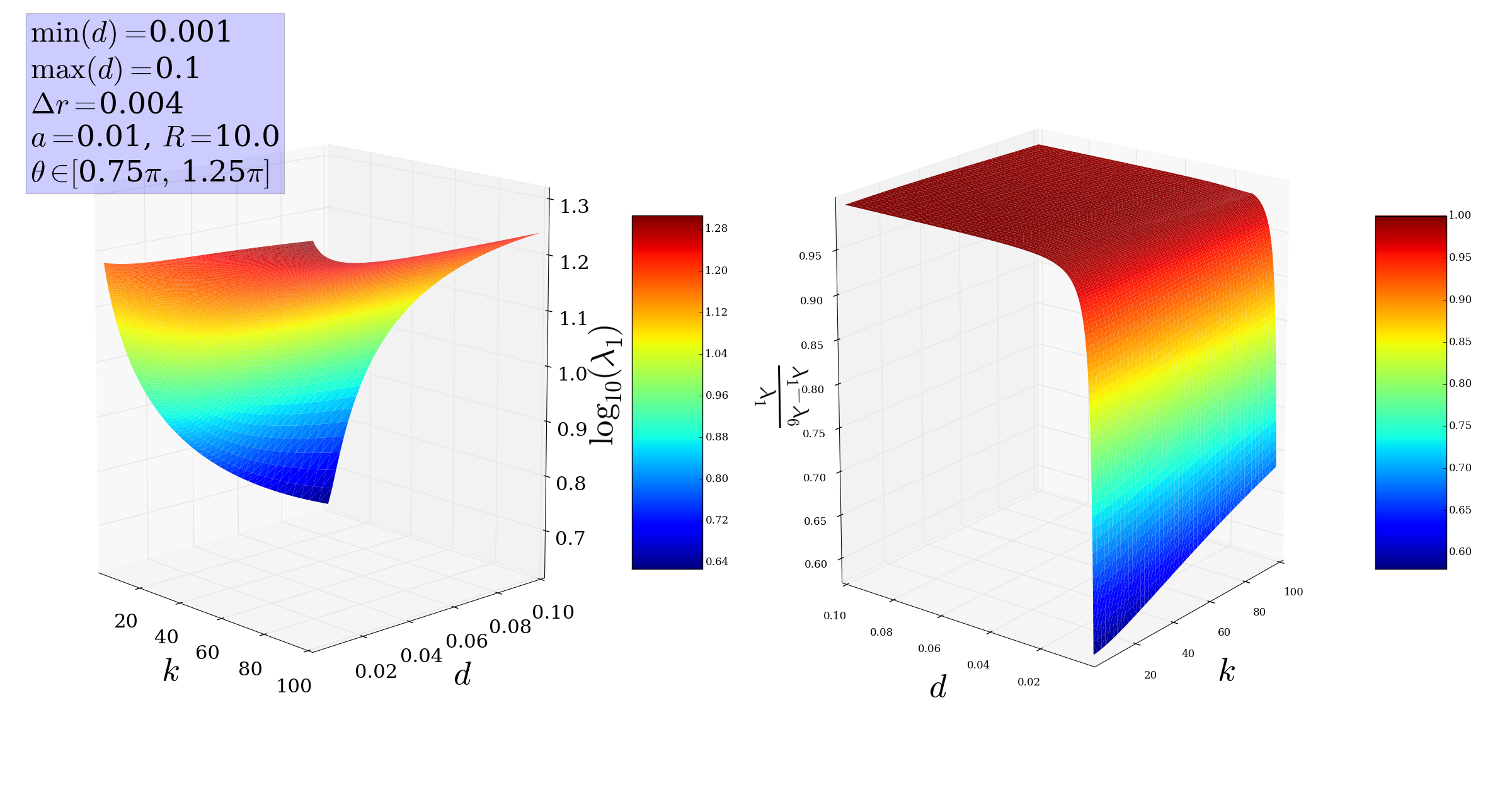
We present below Figure 7, which shows how the first 5050 singular values of the operator K=(K1,K2)K=(K_{1},K_{2}) vary with dd. It is clear that for dd small (i.e. for control in the nearfield of the antenna), the rate of decay of the singular values of KK is considerably slower than for larger dd. This in turn provides some experimental evidence for the fact that nearfield control seems to be more feasible in terms of stable dependence of the solution ϕ\phi on ff. We also show Figure 8, which shows the behavior of the first and sixth singular value of KK with respect to dd and kk.

Refer to caption
Figure 7: Plot of first 5050 singular values of K:L2​(∂Da)→ΞK:L^{2}(\partial D_{a})\to\Xi for ∂Da\partial D_{a} a circular antenna of radius a=0.01a=0.01 and ∂Dc\partial D_{c} an annular region of varying distance from ∂Da\partial D_{a}.
Refer to caption
Figure 8: Plot of first singular value of K:L2​(∂Da)→ΞK:L^{2}(\partial D_{a})\to\Xi as well as the relative difference of the first and sixth singular values with respect to dd and kk. Again, ∂Da\partial D_{a} is a circular antenna of radius a=0.01a=0.01 and ∂Dc\partial D_{c} an annular region.

4.3 Control for a Spherical Point Source

We now consider the case that

f1​(𝐱)=i4​H0(1)​(k​|𝐱−𝐱0|),f_{1}(\mathbf{x})=\frac{i}{4}H_{0}^{(1)}(k|\mathbf{x}-\mathbf{x}_{0}|),

where 𝐱0\mathbf{x}_{0} is the source point. In all examples presented in this section, we have R=10R=10 unless otherwise noted, and 𝐱0=[20,0]T\mathbf{x}_{0}=[20,0]^{T} or 𝐱0=[10000,0]T\mathbf{x}_{0}=[10000,0]^{T} (to approximate a source at infinity).

First we observe how the frequency kk and distance dd from ∂Dc\partial D_{c} to ∂Da\partial D_{a} affects the various control criteria. In figures 9 and 10 we vary kk from 0.10.1 to 100100 and dd from 0.0010.001 to 0.0030.003 with a=0.01a=0.01. With the error discrepancy set at δ=0.02\delta=0.02, we have in both figures that relative error on ∂Dc\partial D_{c} is very close to 2%2\% for all data points. Moreover, with 0.5%0.5\% noise added to ff, roughly a 5%5\% change in ϕ\phi is observed at all frequencies when dd is near its lower limit. A bit more sensitivity is observed for frequencies k<20k<20 when dd increases beyond 0.010.01. Interestingly, for k>20k>20 the optimal parameter α\alpha is larger and corresponding power budget smaller in order to achieve discrepancy δ\delta.

Refer to caption
Figure 9: Plot vs. kk and dd for f1f_{1} a spherical point source at 𝐱0=[10000, 0]T\mathbf{x}_{0}=[10000,\,0]^{T}.
Refer to caption
Figure 10: Plot vs. kk and dd for f1f_{1} a spherical point source at 𝐱0=[20, 0]T\mathbf{x}_{0}=[20,\,0]^{T}.

In figures 9 and 10 it is clear that for smaller dd values the sensitivity of ϕ\phi to 0.5%0.5\% noise added to ff is close to 5%5\%. As dd increases, sensitivity of ϕ\phi to noise increases as expected. Having 𝐱0\mathbf{x}_{0} nearer or farther from ∂BR\partial B_{R} does not have a very significant effect on the overall shape of each subplot.

Refer to caption
Figure 11: Plot vs. dd and ϵ\epsilon for f1f_{1} a spherical point source at 𝐱0=[10000, 0]T\mathbf{x}_{0}=[10000,\,0]^{T}.
Refer to caption
Figure 12: Plot vs. dd and ϵ\epsilon for f1f_{1} a spherical point source at 𝐱0=[20, 0]T\mathbf{x}_{0}=[20,\,0]^{T}.

Figures 11 and 12 show how the quantities of interest change with dd and the noise factor ϵ\epsilon, both with k=10k=10. The reason for choosing k=10k=10 instead of, e.g., k=1k=1 is that from figure 9 we see a slightly higher sensitivity of ϕ\phi to noise for approximately 1<k<201<k<20 when dd starts to increase. So the goal was to capture the worst case scenario for the control stability. For smaller values of dd we see as before that a roughly 0.5%0.5\% change in f1f_{1} yields about a 5%5\% change in ϕ\phi. Moreover, the dependence on ϵ\epsilon for fixed dd is superlinear, consistent with the illposedness of the problem. Interestingly, sensitivity of ϕ\phi at d≈0.015d\approx 0.015 is better than at nearby values, but of course such a value depends on the other parameters of the problem setup.

Refer to caption
Figure 13: Plot vs. kk and RR for f1f_{1} a spherical point source at 𝐱0=[10000, 0]T\mathbf{x}_{0}=[10000,\,0]^{T}.

Finally, we consider Figure 13, which shows the dependence on RR and kk for a source at 𝐱0=[10000, 0]T\mathbf{x}_{0}=[10000,\,0]^{T}. Overall, one can see that RR can be decreased to around R=3R=3 at any frequency between 0.10.1 and 100100 and still achieve the same approximate level of sensitivity for ϕ\phi as in the previous plots with R=10R=10.

5 Conclusions and Future Work

In this paper we studied the feasibility of the active control scheme for the scalar Helmholtz equation. In the L2L^{2} setting, we presented analytic conditional stability results as well as detailed numerical sensitivity studies for the minimal energy solution. We provided several analytic and numerical arguments for the scheme’s feasibility and broadband character in the near field when the interrogating field is a far field of a far field observer.

We focused our discussion in this paper only on the case of an interrogating far field point source (i.e. similar to a plane wave with corresponding decay) because we believe that this situation is relevant in usual radar or sonar detection problems. In contrast, the case of an interrogating plane wave corresponds to a different problem, where the observer is close to the source and control region and thus the interrogating signal does not have sufficient decay.

In fact, we have numerically studied the case when the interrogating field is a plane wave without decay or a given uniform field. We observed the scheme does not behave well for the uniform field and that although the stability and accuracy of the near field scheme are essentially independent of the plane wave direction, the overall performance of the scheme is not as good when compared to the case of an interrogating signal coming from a far field observer presented above. In fact, for the same settings as in Figure 2 when comparing the case of an interrogating far field point source with an interrogating plane wave, we obtained 5%5\% versus 8%8\% stability error and power budget levels of ≈10−1\approx 10^{-1} versus ≈10\approx 10. We conclude that the scheme performance depends not only on the location of the control region with respect to the source region but also on the amplitude and oscillatory pattern of the incoming field.

Currently we are considering a more localized basis for L2​(∂Da)L^{2}(\partial D_{a}) (e.g. delta function basis, or splines) in order to better observe the field characteristics in the control region DcD_{c} and around the antenna DaD_{a}. We also plan to study the active control scheme for linear arrays and for large elongated antennas. Then, as a next step in our research efforts, we will work on the extension of the current numerical sensitivity study to three dimensions and full Maxwell system and on the study of near field control with planar and conformal arrays.

References

  • [1] Andrea Alú and Nader Engheta. Plasmonic and metamaterial cloaking: Physical mechanisms and potentials. J. Integral Equations Appl., 10(9), 2008.
  • [2] A. Bakushinsky and A. Goncharsky. Ill-posed problems: theory and applications, volume 301 of Mathematics and its Applications. Kluwer Academic Publishers Group, Dordrecht, 1994. Translated from the Russian by I. V. Kochikov.
  • [3] Huanyang Chen and C.T. Chan. Acoustic cloaking and transformation acoustics. J. Phys. D: Appl. Phys., 43(11), 2010.
  • [4] Huanyang Chen, C.T. Chan, and Ping Sheng. Transformation optics and metamaterials. Nature Mater., 9(5):387, 2010.
  • [5] David Colton and Rainer Kress. Inverse Acoustic and Electromagnetic Scattering Theory, volume 93 of Applied Mathematical Sciences. Springer-Verlag, Berlin, second edition, 1998.
  • [6] S.A. Cummer, B.I. Popa, D. Schurig, D.R. Smith, J. Pendry, M. Rahm, and A. Starr. Scattering theory derivation of a 3d acoustic cloaking shell. Phys. Rev. Lett., 100(2), 2008.
  • [7] Junjie Du, Shiyang Liu, and Zhifang Lin. Broadband optical cloak and illusion created by the low order active sources. Optics Express, 20(8):8608–17, 2012.
  • [8] S.J. Elliot and P.A. Nelson. Integral equation methods in scattering theory. Electronics and Comm. Engineering Journal, 2(4):127–136, 1990.
  • [9] Heinz W. Engl, Martin Hanke, and Andreas Neubauer. Regularization of Inverse Problems, volume 375 of Mathematics and its Applications. Kluwer Academic Publishers Group, Dordrecht, 1996.
  • [10] C.R. Fuller and A.H. von Flotow. Active control of sound and vibration. IEEE, 15(6):9–19, 1995.
  • [11] Allan Greenleaf, Yaroslav Kurylev, Matti Lassas, and Gunther Uhlmann. Invisibility and inverse problems. Bull. Amer. Math. Soc. (N.S.), 46(1):55–97, 2009.
  • [12] Allan Greenleaf, Matti Lassas, and Gunther Uhlmann. Anisotropic conductivities that cannot be detected by eit. Physiol. Meas, 24(2), 2003.
  • [13] Allan Greenleaf, Matti Lassas, and Gunther Uhlmann. On nonuniqueness for Calderón’s inverse problem. Math. Res. Lett., 10(5-6):685–693, 2003.
  • [14] Fernando Guevara Vasquez, Graeme W. Milton, and Daniel Onofrei. Active exterior cloaking for the 2d laplace and helmholtz equations. Physical Review Letters, 103(7):073901+, August 2009.
  • [15] Fernando Guevara Vasquez, Graeme W. Milton, and Daniel Onofrei. Broadband exterior cloaking. Opt. Express, 17(17):14800–14805, Aug 2009.
  • [16] Fernando Guevara Vasquez, Graeme W. Milton, and Daniel Onofrei. Exterior cloaking with active sources in two dimensional acoustics. Wave Motion, 48(6):515–524, 2011. Special Issue on Cloaking of Wave Motion.
  • [17] Fernando Guevara Vasquez, Graeme W. Milton, Daniel Onofrei, and Pierre Seppecher. Transformation elastodynamics and active exterior acoustic cloaking. In Richard V. Craster and Sébastien Guenneau, editors, Acoustic Metamaterials, volume 166 of Springer Series in Materials Science, pages 289–318. Springer Netherlands, 2013.
  • [18] Tosio Kato. Perturbation Theory for Linear Operators. Classics in Mathematics. Springer-Verlag, Berlin, 1995. Reprint of the 1980 edition.
  • [19] Andreas Kirsch. An introduction to the mathematical theory of inverse problems, volume 120 of Applied Mathematical Sciences. Springer, New York, second edition, 2011.
  • [20] Rainer Kress. Linear Integral Equations, volume 82 of Applied Mathematical Sciences. Springer, New York, third edition, 2014.
  • [21] Yun Lai, Huanyang Chen, Zhao Q. Zhang, and C.T. Chan. Complementary media invisibility cloak that cloaks objects at a distance outside the cloaking shell. Physical Review Letters, 102:093901+, March 2009.
  • [22] Ulf Leonhardt. Notes on conformal invisibility devices. New Journal of Physics, 8(118), July 2006.
  • [23] Ulf Leonhardt. Optical conformal mapping. Science, 312(5781):1777–1780, June 2006.
  • [24] J. Loncaric, V.S. Ryaben’kii, and S.V. Tsynkov. Active shielding and control of environmental noise. Technical report, Institute for Computer Applications in Science and Engineering (ICASE), 2000.
  • [25] J. Loncaric and S.V. Tsynkov. Quadratic optimization in the problems of active control of sound. Applied Numerical Mathematics, 52(4):381–400, 2005.
  • [26] Paul Lueg. Process of silencing sound oscillations, June 1936. US Patent 2,043,416.
  • [27] Qian Ma, Zhong Lei Mei, Shou Kui Zhu, Tian Yu Jin, and Tie Jun Cui. Experiments on active cloaking and illusion for laplace equation. Phys. Rev. Lett., 111:173901, Oct 2013.
  • [28] E.A. Marengo and A.J. Devaney. The inverse source problem of electromagnetics: linear inversion formulation and minimum energy solution. Antennas and Propagation, IEEE Transactions on, 47(2):410–412, Feb 1999.
  • [29] David A. B. Miller. On perfect cloaking. Opt. Express, 14(25):12457–12466, Dec 2006.
  • [30] Graeme W. Milton and Nicolae-Alexandru P. Nicorovici. On the cloaking effects associated with anomalous localized resonance. Proc. R. Soc. Lond. Ser. A Math. Phys. Eng. Sci., 462(2074):3027–3059, 2006.
  • [31] G.W. Milton, N.-A. P. Nicorovici, R.C. McPhedran, K. Cherednichenko, and Z. Jacob. Solutions in folded geometries, and associated cloaking due to anomalous resonance. New Journal of Physics, 10, Nov 2008.
  • [32] N.-A. P. Nicorovici, G.W. Milton, R.C. McPhedran, and L.C. Botten. Quasistatic cloaking of two-dimensional polarizable discrete systems by anomalous resonance. Opt. Express, 15(10):6314–6323, May 2007.
  • [33] Andrew N. Norris, Feruza A. Amirkulova, and William J. Parnell. Source amplitudes for active exterior cloaking. Inverse Problems, 28(10):105002, 20, 2012.
  • [34] Harry F. Olson and Everett G. May. Electronic sound absorber. The Journal of the Acoustical Society of America, 25(4):829–829, 1953.
  • [35] Daniel Onofrei. On the active manipulation of fields and applications: I. The quasistatic case. Inverse Problems, 28(10):105009, 15, 2012.
  • [36] Daniel Onofrei. Active manipulation of fields modeled by the Helmholtz equation. J. Integral Equations Appl., 26(4):553–579, 2014.
  • [37] N. Peake and D.G. Crighton. Active control of sound. Annual Review of Fluid Mechanics, 32(1):137–164, 2000.
  • [38] J.B. Pendry, D. Schurig, and D.R. Smith. Controlling electromagnetic fields. Science, 312(5781):1780–1782, 2006.
  • [39] A.W. Peterson and S.V. Tsynkov. Active control of sound for composite regions. SIAM J. Appl. Math., 67(6):1582–1609, 2007.
  • [40] M. Selvanayagam and G.V. Eleftheriades. An active electromagnetic cloak using the equivalence principle. Antennas and Wireless Propagation Letters, IEEE, 11:1226–1229, 2012.
  • [41] Michael Selvanayagam and George V. Eleftheriades. Experimental demonstration of active electromagnetic cloaking. Phys. Rev. X, 3:041011, Nov 2013.
  • [42] H.H. Zheng, J.J. Xiao, Y. Lai, and C.T. Chan. Exterior optical cloaking and illusions by using active sources: A boundary element perspective. Phys. Rev. B, 81:195116, May 2010.