The Missing Link: Bayesian Detection and Measurement of Intermediate-Mass Black-Hole Binaries

In this study we employ nonspinning waveforms constructed within the effective-one-body (EOB) formalism [48, 49] and calibrated to highly-accurate numerical relativity (NR) simulations having typical length of $30\mbox{--}40$ GW cycles and mass ratios $q\leq 6$ [5]. More specifically, we use the EOBNRv2HM code in the LIGO Algorithm Library (LAL) [50] to generate the EOB waveform model in Ref. [5], which includes four subleading modes, namely the $(l,m)=(2,1)$, $(3,3)$, $(4,4)$ and $(5,5)$ modes, as well as the leading $(l,m)=(2,2)$ mode ²² 2 An EOB model with different parametrization was subsequently calibrated to the same set of NR waveforms used in Ref. [5] and provides two subleading modes $(l,m)=(2,1)$ and $(3,3)$ [51], besides the leading one.. [These modes come from the decomposition of the GW signal $h=h_{+}-\imath h_{\times}$ into $-2$ spin-weighted spherical harmonics ${}_{-2}Y_{lm}$ [5].] Consequently, GW signals that we study contain the first five harmonics of the orbital frequency. During most of the early inspiral phase only the $(2,2)$ mode, and, in particular, its Newtonian amplitude, will be the dominant component. Other harmonics and PN corrections become increasingly important as we get close to merger. The effect of these higher modes is especially relevant when the binary in question has its merger and ringdown frequencies in the most sensitive part of a detector’s response. The ringdown frequency of the final remnant of binaries consisting of nonspinning BHs of total mass 50 $\mathrm{M}_{\odot}$ to 500 $\mathrm{M}_{\odot}$ varies over the range 40 Hz to 400 Hz—the frequency range where LIGO and Virgo have the best sensitivity, and this provides the motivation for our choice of masses used in this study.

A Markov-chain Monte-Carlo (MCMC) study [32] demonstrated that the EOB waveforms of Ref. [5] are indistinguishable from the NR waveforms [52] used to calibrate them up to $\mathrm{SNR}=50$ for advanced LIGO detectors. Subsequent investigations carried out in Ref. [53] verified the accuracy of these nonspinning EOB waveforms in the entire sensitivity band of advanced LIGO detectors and suggested that the EOB model be accurate even outside the region of calibration, i.e. when $q>6$. This expectation was verified by the very good agreement found against the $q=10$ NR waveform of $20$ GW cycles in Ref. [54] and, especially, against the $q=7$ NR waveform of $350$ GW cycles recently produced by the SXS collaboration [55].

Since in our study we consider BBHs in quasi-circular orbits with negligible spins, the system can be described by nine parameters: $\bm{\theta}=\{m_{1},m_{2},d_{L},t_{c},\delta,\alpha,\theta_{\rm JN},\psi,\phi\}$. The parameters $m_{1}$ and $m_{2}$ are the masses of the individual BHs. From these quantities we define the total intrinsic mass, $M=(m_{1}+m_{2})$, the total observed mass, $M_{\mathrm{obs}}=M\,(1+z)$ with $z$ being the redshift, the mass ratio, $q=m_{1}/m_{2}\geq 1$, the symmetric mass ratio, $\eta=m_{1}m_{2}/(m_{1}+m_{2})^{2}=q/(1+q)^{2}$, the intrinsic chirp mass, $\mathcal{M}=M\eta^{3/5}$ and the observed chirp mass, $\mathcal{M}_{\rm obs}=\mathcal{M}\,(1+z)$. The parameter $d_{L}$ is the luminosity distance and when combined with the declination $\delta$ and right ascension $\alpha$, it defines the sky location of the binary. The time of the peak in the $(2,2)$ mode of the waveform, as measured at the geocenter, is given by $t_{c}$; this serves as an approximation of the merger time. The angle $\theta_{\rm JN}$ measures the inclination of the binary’s total angular momentum $\mathbf{J}$ (equal to the orbital angular momentum, $\mathbf{L}$, as the holes are non-spinning) with respect to the line of sight from the detectors $\mathbf{n}$ (geocenter). The polarization $\psi$ and the phase $\phi$ provide the additional Euler angles necessary to describe the rotation from $\mathbf{n}$ to $\mathbf{J}$.

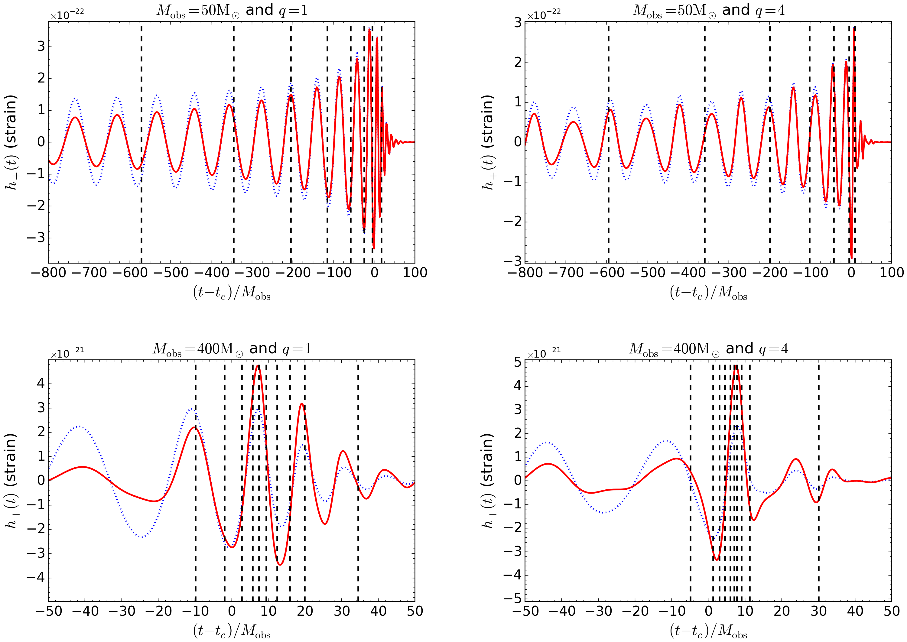
In this paper we are interested in studying the effect on parameter estimation of binary systems with larger and larger total masses. When we maintain a constant SNR and increase the binary’s total mass, the signal moves downward in frequency space, resulting in more power from the merger and ringdown portions as opposed to the inspiral. The merger occurs at approximately the frequency of the last stable orbit (LSO), which in the case of a Schwarzschild BH is $f_{\rm LSO}\simeq 4400\,(\mathrm{M}_{\odot}/M)\textrm{Hz}.$ We begin our integration at $f_{\rm min}=10\,\textrm{Hz}$, so for systems with $M_{\mathrm{obs}}\geq 400\mathrm{M}_{\odot}$ there will be little power from the inspiral portion of the waveform. As the inspiral evolution is dominated by $\mathcal{M}_{\rm obs}$ and the merger and ringdown are dominated by $M_{\mathrm{obs}}$, we expect the character of the parameter estimation to transition from one to the other (see Sec. V).

To demonstrate this expectation, we compare in Fig. 2 two waveforms with $M_{\mathrm{obs}}=50\mathrm{M}_{\odot}$ and $400\mathrm{M}_{\odot}$. We show both the original waveform and the waveform normalized by the advanced LIGO zero-detuned high-power (ZDHP) power spectral density (PSD), $S_{n}(f)$; the normalized waveform has been re-scaled so that it has the same amplitude at $t=0$ as the original. The comparisons clearly show that for the $(M_{\mathrm{obs}},q)=(50\mathrm{M}_{\odot},1)$ waveform, $90\%$ of the power (SNR²) has been accumulated during the inspiral and that the merger and ringdown play only a minor role. On the other hand, for the $(M_{\mathrm{obs}},q)=(400\mathrm{M}_{\odot},1)$ waveform, only $10\%$ of the power is collected during the inspiral and now the merger and ringdown are predominant features. In Fig. 3 we show the amplitudes of the waveforms in frequency space in comparison to the advanced LIGO ZDHP and advanced Virgo design $\sqrt{S_{n}(f)}$. We can see in Fig. 3 that for the higher-mass waveforms, the entire inspiral signal is strongly down-weighted by the rising of the amplitude spectral density with the merger occurring as $\sqrt{S_{n}(f)}$ reaches a minimum. For the lower-mass waveforms, much of the inspiral is in the frequency band where the amplitude spectral density is at or near minimum, thereby allowing this part of the waveform to dominate.

Bayesian inference provides a statistically rigorous method of measuring the probability distribution of a set of parameters $\bm{\theta}$ given a model or hypothesis $\mathcal{H}$ and a set of data $\mathcal{D}$. Bayes’ theorem states that

where $\Pr(\bm{\theta}|\mathcal{D},\mathcal{H})$ is the posterior probability distribution of parameters used for making inferences about which signal parameters $\bm{\theta}$ best fit the data and what the corresponding credible regions are; $\Pr(\mathcal{D}|\bm{\theta},\mathcal{H})$ is the likelihood of obtaining the data given the specific model and parameters, for which we use the shorthand $\mathcal{L}(\bm{\theta})$; $\Pr(\bm{\theta}|\mathcal{H})$ is the prior probability of the parameters for the model that represents our knowledge of these values before looking at the data (a priori); and $\Pr(\mathcal{D}|\mathcal{H})$ is the Bayesian evidence, which is commonly abbreviated as $\mathcal{Z}$. The evidence is the factor needed to normalize the posterior distribution and can therefore also be expressed as

where $N$ is the dimensionality of the parameter space. Since $\mathcal{Z}$ is independent of the parameters, it can be safely ignored for parameter estimation problems, but it is still useful in model comparison.

When comparing two models, $\mathcal{H}_{0}$ and $\mathcal{H}_{1}$, one can write their relative probabilities as

where we used Bayes’ theorem again and have cancelled out $\Pr(\mathcal{D})$ and substituted in $\mathcal{Z}_{i}=\Pr(\mathcal{D}|\mathcal{H}_{i})$ as appropriate. The relative probability of the two models is thus the ratio of their Bayesian evidences multiplied by the relative probability prior to considering the data. In our analysis, we will take the latter to be $1$ and consider the ratio of the Bayesian evidences, which is called the odds ratio. In the problem of signal detection, $\mathcal{H}_{0}$ can be considered the noise-only model while $\mathcal{H}_{1}$ is the signal-plus-noise model. Therefore, an odds ratio much greater than $1$ indicates a strong belief in the presence of a signal. This method naturally incorporates Occam’s razor, such that more complicated models are penalized and must sufficiently improve the fit to the data to be favored.

Nested sampling [56] is a Bayesian inference technique developed for the calculation of the evidence, through which posterior probability samples are produced as a by-product. This is done by transforming the $N$-dimensional integral for $\mathcal{Z}$ into a $1$-dimensional integral over the prior volume. We define the prior volume $X$ by $dX=\Pr(\bm{\theta}|\mathcal{H})d^{N}\bm{\theta}$. We can therefore write the prior probability volume enclosed within a contour (in parameter space) of constant likelihood $\lambda$ as

The evidence integral of Eq. (2) can be re-written as

where $L(X)$ is the inverse of Eq. (4) (returns the likelihood at which a prior volume of $X$ is enclosed) and is a monotonically decreasing function of $X$ (i.e. more prior volume implies lower likelihood contour bound). If we can evaluate likelihood values $L_{i}=L(X_{i})$ such that $X_{i}$ is a sequence of monotonically decreasing values, the evidence can be computed as a simple sum

Here, the $w_{i}$ are weights which can be taken from a simple trapezium rule such that $w_{i}=\tfrac{1}{2}(X_{i-1}-X_{i+1})$.

The individual prior weight of each sampled point can also be estimated from the sequence of $X_{i}$ values. This may be combined with the computed likelihood for that point and the evidence to produce a final posterior probability for the point. The full sequence of points can then be re-sampled accordingly to the points’ individual probabilities to produce a set of samples from the posterior.

Nested sampling operates by starting with an initial set of ‘live’ points sampled from the prior distribution. Iterations are then performed whereby the point with lowest likelihood value is removed from the live point set and a new point is sampled from the prior with the restriction that it has higher likelihood than the point just removed. This removal and replacement is continued until a stopping condition is reached (e.g., a tolerance on the evidence calculation). The difficult task here lies in the efficient sampling of new points under this restriction. As the likelihood contour moves upwards, the volume of the prior within that contour will decrease to very small values, making direct sampling of the prior very inefficient. The MultiNest algorithm [57, 58, 59] addresses this by enclosing the live points in clusters of ellipsoids. A new sample can then be made from the ellipsoids very quickly and as they shrink along with the live points, they create effective likelihood contours to be sampled from, thereby greatly increasing the sampling efficiency. The ellipsoids can be distributed to enclose degenerate and multimodal distributions, making this approach very robust.

MultiNest is implemented within BAMBI [60], which is linked with the LALInference [61] code of LAL. The lalinference_bambi sampler is used for analysis of simulated signals in this study.

The priors used in this analysis are flat in the component masses, with $\{m_{1},m_{2}\}\in[10,600]\,\mathrm{M}_{\odot}$ and $m_{1}\geq m_{2}$. In Section V.4, we assess the effect of changing the prior by implementing an alternative mass prior that is flat in the log of chirp mass for $\mathcal{M}\in[2.45,435.275]\,\mathrm{M}_{\odot}$ and flat over $\eta\in[0.03,0.25]$.

In both setups, the source location prior is uniform in volume, thus proportional to $d_{L}^{2}$ for $d_{L}\in[100\,\textrm{Mpc},10\,\textrm{Gpc}]$ and flat in $\sin(\delta)$ and $\alpha$ for $\delta\in[0,\pi]\,\textrm{rad}$ and $\alpha\in[0,2\pi)\,\textrm{rad}$. We use a prior flat in coalescence time that is centered on the true value with $\Delta t_{c}\in[-0.1,0.1]\,\textrm{s}$. The orientation angles are assumed to be isotropically distributed, thus flat in $\sin(\theta_{\rm JN})$, $\psi$, and $\phi$ for $\theta_{\rm JN}\in[0,\pi]\,\textrm{rad}$, $\psi\in[0,\pi)\,\textrm{rad}$, and $\phi\in[0,2\pi)\,\textrm{rad}$.

In general, the data obtained from adavanced LIGO and Virgo detectors is the sum of signal, $\mathbf{h}$, and noise, $\mathbf{n}$,

The signal in a given detector is given by

where $\mathbf{h}_{+,\times}$ are the two independent GW polarizations and $\mathbf{F}_{+,\times}(\alpha,\delta,\psi)$ are the antenna response functions [62] that depend on the source location and polarization. The antenna response is slowly varying in time due to the rotation of the Earth, but this effect is small for the short duration of the signals considered in this study ($<2$ min).

The noise is modeled as independent and Gaussian in each frequency with a mean of zero and variance given by the detector’s PSD. Therefore, the probability of a data stream, $\mathbf{d}_{a}$, in detector $a$ containing a given signal, $\mathbf{h}(\bm{\theta})$, is given by the probability of the resulting noise realization, $\mathbf{n}=\mathbf{d}-\mathbf{h}(\bm{\theta})$. This is given by the product (sum in log-space) of the probability of the noise for each frequency bin [61]:

where $T$ is the segment length, the tilde indicates the discrete Fourier transform of the function, and $i$ is an index over frequency bins. The noise power spectral density $S_{n}(f)$ will vary from detector to detector and here we use the ones at design sensitivity for advanced LIGO and Virgo [22]³³ 3 See https://dcc.ligo.org/LIGO-P1200087-v19/public for PSD data files. $H_{s}$ indicates that we are using the signal model that assumes a signal is present; this will be compared to the noise-only model, $H_{n}$, where $\mathbf{h}=\mathbf{0}$. The final likelihood is the product of likelihoods from the individual detectors,

To simulate the sensitivity for advanced LIGO and Virgo detectors, we use a minimum frequency of $f_{\textrm{min}}=10\,\textrm{Hz}$. In order to include the highest ringdown mode for the lowest possible total mass system, we use a sampling rate of $4096\,\textrm{Hz}$, giving a Nyquist frequency of $f_{\textrm{Nyq}}=2048\,\textrm{Hz}$ for the upper bound of our likelihood sum. A segment length of $128\,\textrm{s}$ ensures that no waveforms are cutoff in-band.

In our first set of comparisons, we study the effect of the total mass of the system on the estimation of the source’s intrinsic parameters. Specifically, we investigate the statistical errors on the measurement of $M_{\mathrm{obs}}$, $\mathcal{M}$, $\eta$, $m_{1}$, and $m_{2}$. Posterior distributions over $(M_{\mathrm{obs}},\mathcal{M}_{\rm obs})$-space and $(m_{1},m_{2})$-space are shown for various values of $M_{\mathrm{obs}}$ (always using $q=4$ and $\theta_{\rm JN}=\pi/3$) in Fig. 6. These are summarized in the left panel of Fig. 7, which shows the relative widths of the $95\%$ ($\pm 2\mbox{-}\sigma$) credible intervals (i.e., $(x_{97.5\%}-x_{2.5\%})/x_{\rm true}$) for the various mass parameters. At the lower mass end ($M_{\mathrm{obs}}=50\mathrm{M}_{\odot}$), uncertainty is low due to how well the chirp mass $\mathcal{M}_{\rm obs}$ is measured from the inspiral phase of a waveform. As the total mass increases, the uncertainty increases and for $M_{\mathrm{obs}}\geq 150\mathrm{M}_{\odot}$ the uncertainty in $\mathcal{M}_{\rm obs}$ is similar to or greater than that in $M_{\mathrm{obs}}$. This change is due to less inspiral signal being present in the most sensitive band of the detector; the ringdown is predominantly dependent on $M_{\mathrm{obs}}$ and therefore this parameter is measured more accurately. However, the inspiral measures $\mathcal{M}_{\rm obs}$ better than the ringdown measures $M_{\mathrm{obs}}$, so the resulting uncertainty is larger. Above $M_{\mathrm{obs}}=300\mathrm{M}_{\odot}$, the uncertainty decreases slightly; this is due to the ringdown matching up better with the minimum of the advanced LIGO/Virgo PSD and the subleading modes moving into more sensitive regions of the PSD.

When these same systems are face-on ($\theta_{\rm JN}=0$) or have lower $q$ (more equal component masses), the uncertainties for the $(2,2)$-only waveform closely resemble those for the waveform with all modes, just a little larger. This can be seen in the right panel of Fig. 7 and it is what would be expected for systems with little contribution from the subleading modes. In all cases, the templates that include subleading modes of radiation have lower uncertainty than those using only the $(2,2)$ mode. Additionally, for inclined and asymmetric systems, as $M_{\mathrm{obs}}$ increases from $300\mathrm{M}_{\odot}$ to $500\mathrm{M}_{\odot}$, the uncertainty when using $(2,2)$-only templates grows significantly while that from using templates with subleading modes slightly decreases. This is due to the fact that the subleading modes provide information about the mass ratio of the system in their relative amplitudes and phases. This information contained in the subdominant modes breaks the model degeneracies and allows us to better infer the component masses as the ringdown phase of the waveform enters the most sensitive region of the PSD. These results can also be seen in Fig. 6. Being able to accurately measure the component masses is important in allowing us to make inferences on the source population of these massive BHs [8].

Thus, we observe that at an SNR of $12$ uncertainties for $M_{\mathrm{obs}}$ can reach $\sim 20\mbox{--}25\%$ in asymmetric binaries while uncertainty in $\mathcal{M}_{\rm obs}$ reaches up to $\sim 50\mbox{--}60\%$ (these numbers are $\sim 17\%$ versus $\sim 22\%$ in more symmetric mass ratio binaries).

In Appendix A, we provide summary tables of relative $95\%$ credible intervals for measurements of the masses, luminosity distance, and coalescence time. These are given over a range of SNRs for two mass ratios ($q=\{1.25,4\}$) and several observed total masses at the inclinations of $\theta_{\rm JN}=\{\pi/3,0\}$.

As the IMBHB systems increase in total mass, there are distinct changes in the two-dimensional posterior probability distributions. As the inspiral phase evolution strongly constrains $\mathcal{M}_{\rm obs}$ and $\eta$, in that order, lower mass systems will have degeneracies that follow contours in these parameters. With increasing total mass, however, the inspiral becomes less important and the merger-ringdown part of the signal contributes significantly or dominantly to the SNR. This is most well described by $M_{\mathrm{obs}}$ with much weaker dependence on $\eta$. Thus, we expect there to be a change in the degeneracies present in the mass estimation. The inspiral dependency on $\mathcal{M}_{\rm obs}$ can be seen in the PN inspiral waveforms (see Ref. [71]); PN approximants are accurate for early inspiral when the BHs are sufficiently far from merger. The dependency on $M_{\mathrm{obs}}$ of the ringdown is similarly given by the quasi-normal mode decomposition derived in Ref. [72] and implemented in the EOB waveform models used in our study [5].

This change in the optimally measured parameters as $M_{\mathrm{obs}}$ increases can be observed in Fig. 6. In the right column, we show the posterior distribution of the masses, parameterized as $M_{\mathrm{obs}}$ and $\mathcal{M}_{\rm obs}$, over a range of total masses for an asymmetric system ($q=4$, $\eta=0.16$) viewed at an angle ($\theta_{\rm JN}=\pi/3$). In the top row, $M_{\mathrm{obs}}=50\mathrm{M}_{\odot}$ and we can see that the principal measurement is of the chirp mass $\mathcal{M}_{\rm obs}$ – posterior samples and contours lie along a line of near-constant $\mathcal{M}_{\rm obs}$. As $M_{\mathrm{obs}}$ increases, at $M_{\mathrm{obs}}=150\mathrm{M}_{\odot}$ a second principal direction of degeneracy becomes evident. This is due to a different combination of the mass parameters becoming increasingly constrained relative to the others and realizing a new degeneracy in the measurement.

These observations confirm what we see in the one-dimensional posteriors in Fig. 7. The chirp mass $\mathcal{M}_{\rm obs}$ is initially measured to lower fractional error than the total mass $M_{\mathrm{obs}}$; as $M_{\mathrm{obs}}$ increases the uncertainty grows much faster in $\mathcal{M}_{\rm obs}$ than it does in $M_{\mathrm{obs}}$. The small decrease in uncertainty at the higher masses is also visible as the contours shrink slightly. We are now able to see in Fig. 6 that this increase in uncertainty is accompanied by a changing of the dominant degeneracy in the parameters of the waveform model.

As discussed previously, in addition to the leading $(2,2)$ mode, the EOBNRv2HM waveform model also includes subleading modes $(2,1)$, $(3,3)$, $(4,4)$, and $(5,5)$, which introduce additional structure to the waveform and improve faithfulness to NR waveforms. This increased structure is important as the relative amplitudes and phasing of the additional modes introduce information about the source masses. In the ringdown phase, the additional modes further constrain the mass and spin of the final BH. This structure creates variation in waveforms as initial component masses are varied, thereby allowing Bayesian inference to measure the masses more accurately and precisely as seen in Figs. 7, 8, and 9.

The modes’ structure also contains angular dependence on the inclination of the system to the detector, $\theta_{\rm JN}$, the orientation of the orbit in the plane of the sky (polarization), $\psi$, and the orbital phase of the binary, $\phi$. This structure is present for the primary $(2,2)$ mode, but the introduction of additional modes breaks degeneracies in the observed waveform as these angles vary.

Improvements in measurement of the masses and orientation angles can all be observed in the example presented in Fig. 8. This figure compares one-dimensional posterior distributions for the case of an injected signal with $M_{\mathrm{obs}}=500\mathrm{M}_{\odot}$, $q=4$, and $\theta_{\rm JN}=\pi/3$. The solid black line shows the posterior distribution for the waveform template model including subleading modes (EOBNRv2HM) and the dashed line is for the waveform template model including only the leading $(2,2)$ mode (EOBNRv2). In both cases, the signal injected into the data contained the subleading modes – in nature, all modes of radiation are present.

For parameter estimation, the presence of subleading modes means that as the angles $\theta_{\rm JN}$, $\psi$, and $\phi$ vary, there is increased variation of the waveform. This variation is more prominent for unequal mass binaries and binaries not observed face-on or face-off ($\theta_{\rm JN}=\{0,\pi\}$), as the subleading modes will have more significant contributions to the SNR. The increased variation allows for more accurate measurement of $\theta_{\rm JN}$ and breaks degeneracies in $\psi$ and $\phi$ to allow these two angles to be measured. As $M_{\mathrm{obs}}$ and $\theta_{\rm JN}$ are strongly correlated with the luminosity distance $d_{L}$ via the amplitude of the waveform, measuring the former two more accurately means that the latter will be measured more accurately as well.

The measurement of the coalescence time $t_{c}$ is offset when using only the leading mode; this is likely due to slight errors in measuring the sky position of the source and adjustments in order to align the peak amplitude of the waveform at merger.

With the additional information provided by the subleading modes in the EOBNRv2HM model, posterior distributions for all mass parameters are narrower and better centered on the true values. Most notably, the subleading modes and their relative amplitudes differentiate better between waveforms with the same total mass, but different mass ratios. The system injected in the analysis shown in Fig. 8 has very high $M_{\mathrm{obs}}$ so the merger and ringdown provide the majority of the SNR. The observed improvement is thus due to a waveform degeneracy in the mass of the final BH that can be broken when we are able to measure the final mass and spin of the BH more precisely. These depend strongly on the mass ratio of the initial components and are further realized in the relative amplitudes of the subleading modes. The improved measurement of initial mass values from using subleading modes can also be seen in Fig. 9, where we compare two-dimensional posteriors in the masses between EOBNRv2HM and EOBNRv2 waveform models over a range of $M_{\mathrm{obs}}$ ($q=4$ and $\theta_{\rm JN}=\pi/3$). Note that when $M_{\mathrm{obs}}=100\mathrm{M}_{\odot}$, the posteriors are nearly identical. However, with increasing $M_{\mathrm{obs}}$, the late inspiral, merger, and ringdown become increasingly important. The parameter estimation bias and loss of SNR is evident when using only the leading mode as the posteriors do not necessarily peak at or strongly support the true values and the confidence intervals are considerably larger.

As the observed total mass increases, it is very difficult to measure the mass ratio $q$ (or $\eta$) if the source is face-on. Indeed, in this case the subdominant modes are not significant; we find that the posteriors are identical and do not change much with respect to the true $q$. However, when $\theta_{\rm JN}=\pi/3$ or $\pi/2$, because of the presence of the subleading modes, it is possible to measure $q$, although the influence of the prior is still evident in tending towards smaller values. In Ref. [8], the authors determine that IMBHBs formed from stellar-origin massive BHs will likely have mass ratios $q\leq 1.25$. We find that for values of $q\geq 2$, in more massive ($M_{\mathrm{obs}}\geq 300\mathrm{M}_{\odot}$) and inclined systems, we will be able to say that $q>1.25$ with certainty $>90\%$.

In summary, we find that the inclusion of subleading modes of gravitational radiation improves the accuracy and precision of the estimation of the source mass parameters as well as some extrinsic parameters, such as distance and orientation angles. They are significant for asymmetric and inclined binaries where they contribute more to the signal’s SNR.

So far, in all of the analysis runs, we have used a very large prior on the component masses, which was flat in $(m_{1},m_{2})$ space. However, one could argue for other reasonable prior distributions on the masses. One such alternative is to use a prior that is flat in $\log(\mathcal{M}_{\rm obs})$. The quantity $\log(\mathcal{M}_{\rm obs})$ is used because $\mathcal{M}_{\rm obs}$ is a scaling factor for the waveform amplitude and $\log(\mathcal{M}_{\rm obs})$ is the so-called Jeffreys prior. Additionally, we employ a prior that is flat in $\eta$ for the second mass parameter.

We ran multiple analyses with this second prior option, which is flat in $(\log(\mathcal{M}_{\rm obs}),\eta)$ and find that even at an SNR of $12$ the strength of the signal is sufficient to render the different prior distribution a minimal factor. This can be seen in Fig.8, where we show the one-dimensional posteriors from a single analysis. More specifically, we display in dotted lines the 1D posteriors of a run with EOBNRv2HM waveform model that uses the alternative prior, to be compared with the solid lines from the run with the original prior. The lines are nearly identical, with differences much smaller than those from using the EOBNRv2 waveform; these differences from the alternative prior will continue to decrease as the SNR is increased.

In an earlier work, Ajith and Bose [30] used inspiral-merger-ringdown phenomenological waveform models (IMRPhenomA) to perform a study similar to ours, but mainly focusing on understanding how uncertainties are reduced when merger and ringdown phases are included. Their study did not include subleading modes. They examined the statistical error in parameter estimation as given by the Fisher information matrix⁴⁴ 4 The Fisher information matrix measures covariances analytically. The square root of the diagonal elements of the inverse of the Fisher matrix gives a lower bound on the standard deviation of the posterior for the parameters. In the limit of large SNR, this estimate becomes exact. and MCMC analyses. Our uncertainties calculated using EOBNRv2 templates ($(2,2)$ mode only) are a factor of a few larger than those given in Table 1 of Ref. [30] for $\textrm{SNR}=10$, $M_{\mathrm{obs}}=\{100,200\}\mathrm{M}_{\odot}$, and $\eta=\{0.25,0.16\}$ (e.g., Ref. [30] quotes relative uncertainties of $2.39\%$ and $3.57\%$ for $M_{\mathrm{obs}}$ in cases with $q=1$ and $M_{\mathrm{obs}}=100\mathrm{M}_{\odot}$ or $M_{\mathrm{obs}}=200\mathrm{M}_{\odot}$; we measure uncertainties of $4.01\%$ and $9.66\%$ in these same cases). The discrepancy in uncertainties is partly a result of the fact that in Ref. [30], the authors maximize their likelihood function over $t_{c}$ and $\phi$ and only perform a single-detector search using an “effective” distance that folds in sky position and binary inclination effects; both of these choices have the effect of fixing values for parameters that we allow to vary in our more general analysis, thus introducing additional uncertainty. Furthermore, we use EOBNRv2HM waveforms as injections, as these most closely model NR waveforms, and our EOBNRv2 templates differ from IMRPhenomA ones, the former being more faithful to NR waveforms [54]. Despite those differences, the quantitative measurements are in general agreement and we also find agreement in the qualitative aspects of increasing uncertainty in mass parameters with increasing $M_{\mathrm{obs}}$. We report our own estimations of the uncertainty in Appendix A, using the full EOBNRv2HM waveform model.

In Ref. [32], Littenberg et al. examined systematic and statistical errors of EOBNR waveforms to assess whether those waveforms are indistinguishable from the NR waveforms used to calibrate them. The authors employed both EOBNRv2 and EOBNRv2HM templates to recover waveforms generated by NR simulations and, when using subleading modes, find systematic errors to be comparable to or less than statistical errors for mass ratios up to $q=6$ and SNRs up to $50$. We find statistical errors comparable to the ones of Ref. [32] for analyses run in common. Our results on the importance of subleading modes for unequal-mass and inclined ($\theta_{\rm JN}>0$) systems reaffirm their findings.

Varma et al. [37] built on Refs. [32, 47]. They used as targets “hybrid” waveforms constructed by attaching PN inspiral/EOB waveforms to NR merger-ringdown waveforms, and as templates EOBNRv2 waveforms. Instead of examining only a few points in parameter space, they ran many simulations in order to average over relative orientation angles. Statistical errors were computed with the Fisher information matrix. Confirming previous work, they found that subleading modes are more important for parameter estimation when $M_{\mathrm{obs}}\geq 150\mathrm{M}_{\odot}$ and $q\geq 4$ and important for detection when $M_{\mathrm{obs}}\geq 100\mathrm{M}_{\odot}$ and $q\geq 6$ (see Fig. 1 of Ref. [37]). In contrast, our paper employs the full EOBNRv2HM waveforms and uses Bayesian analysis, and it extends the study to higher $M_{\mathrm{obs}}$.

Bose et al. [31] focused on the importance of including merger and ringdown phases of the waveform. They analyzed the recovery of inspiral-merger-ringdown waveforms with PN inspiral waveforms and found that at masses as low as $M_{\mathrm{obs}}=50\mathrm{M}_{\odot}$ there are serious systematic errors and an increase in statistical errors due to the loss in SNR. This result is consistent with our analysis showing the significant amount of signal power present in the merger and ringdown phases of the waveform at $M_{\mathrm{obs}}=50\mathrm{M}_{\odot}$ and above.

As mentioned in Sec. I, the merger rate of IMBHBs is currently highly uncertain. Consequently, detection of a single event will immediately confirm the existence of these systems and constrain their rate. In the absence of detection the upper limits reached could be used to rule out some of the models.

As shown in Fig. 1, ground-based detectors will have the greatest distance reach for equal-mass IMBHBs of observed total mass of $\sim 400\mathrm{M}_{\odot}$. The distance reach for such systems will be $\sim 6.5$ Gpc or $z\simeq 1$. We find that the comoving volume averaged over all source orientations and weighted by the antenna pattern functions of the advanced LIGO-Virgo network is $\sim 150\,\mbox{Gpc}^{3},$ larger by a factor $\sim 1.8$ than that in Ref. [8]. This difference can be explained because, as opposed to Ref. [8], we consider a detector network (which increases the reach) and use a different SNR (which decreases the reach). After five years of non-observation of IMBHBs a rate upper limit of $4\times 10^{-11}\,\rm Gpc^{-3}\,yr^{-1}$ can be achieved, which is smaller than the rates for most formation models discussed in Ref. [9, 10, 8]. For a binary of same total mass, $\sim 400\mathrm{M}_{\odot}$, but mass ratio $q=4$, the reach when including subleading modes is smaller by a factor of $1.5$ (see Fig.  1) and the upper limit will be larger by a factor $3.375$, i.e., $1.35\times 10^{-10}\,\rm Gpc^{-3}\,yr^{-1}.$ Neglecting the subleading modes worsens the upper limit by a factor 2.4. However, Ref. [47] showed that in a realistic search the improvement when including subleading modes is significant only for mass ratios larger than $\sim 4$.

An important question in cosmology is the mass function of IMBHs. Routine detection of IMBHs will help us measure the mass function of component BHs that form merging binaries and this should be a proxy for the mass function of IMBHs in the Universe, unless IMBHBs are formed selectively from a sub-population of IMBHs. The component masses of a binary system are strongly correlated and it is not possible to measure them accurately while using only the dominant mode; subleading modes break this degeneracy, especially in the case of asymmetric binaries for which the mass ratio $q$ is large, helping us measure the component masses more accurately. In particular (see Fig. 7), the $95\%$ credible interval in the measurement of the heavier companion can be $10\%$ to $25\%$, while the lighter component is measured within $10\%$ to $125\%$, depending on the total mass of the binary. These results are far better than what might be possible by electromagnetic observations of such binary systems. Therefore, advanced detectors provide the most robust way of determining the mass function across the range of masses from $50\mathrm{M}_{\odot}$ to $500\mathrm{M}_{\odot}$. A related question is the mass function of IMBHBs. Referring to Fig. 7, the total mass is determined to within a few percent in the case of lighter binaries of $50\mathrm{M}_{\odot}$ to within $15\mbox{--}25\%$ for the heaviest systems of $500\mathrm{M}_{\odot}$ that we consider. Thus, advanced detectors should help determine the mass function of IMBHBs.

References

- [1] S. J. Waldman, The Advanced LIGO Gravitational Wave Detector, Tech. Rep. (LIGO Project, 2011).
- [2] J. Aasi et al. (LIGO Scientific Collaboration, Virgo Collaboration), (2013), arXiv:1304.0670 [gr-qc] .
- [3] J. Aasi et al. (LIGO Scientific), Class.Quant.Grav. 32, 074001 (2015), arXiv:1411.4547 [gr-qc] .
- [4] F. Acernese et al. (VIRGO), Class.Quant.Grav. 32, 024001 (2015), arXiv:1408.3978 [gr-qc] .
- [5] Y. Pan, A. Buonanno, M. Boyle, L. T. Buchman, L. E. Kidder, H. P. Pfeiffer, and M. A. Scheel, Phys. Rev. D 84, 124052 (2011).
- [6] A. Buonanno, Y. Chen, and T. Damour, Phys.Rev. D74, 104005 (2006), arXiv:gr-qc/0508067 [gr-qc] .
- [7] P. Ajith, M. Hannam, S. Husa, Y. Chen, B. Bruegmann, et al., Phys.Rev.Lett. 106, 241101 (2011), arXiv:0909.2867 [gr-qc] .
- [8] K. Belczynski, A. Buonanno, M. Cantiello, C. L. Fryer, D. E. Holz, I. Mandel, M. C. Miller, and M. Walczak, ApJ 789, 120 (2014), arXiv:1403.0677 [astro-ph.HE] .
- [9] P. Amaro-Seoane, J. R. Gair, M. Freitag, M. Coleman Miller, I. Mandel, et al., Class. Quant. Grav. 24, R113 (2007), arXiv:astro-ph/0703495 [ASTRO-PH] .
- [10] J. R. Gair, I. Mandel, M. C. Miller, and M. Volonteri, Gen.Rel.Grav. 43, 485 (2011), arXiv:0907.5450 [astro-ph.CO] .
- [11] I. Mandel, J. R. Gair, and M. C. Miller, in Twelfth Marcel Grossmann Meeting on General Relativity (2012) p. 1676, arXiv:0912.4925 [astro-ph.CO] .
- [12] M. Volonteri, Science 337, 544 (2012a), arXiv:1208.1106 [astro-ph.CO] .
- [13] R. Fender and T. Belloni, Science 337, 540 (2012), arXiv:1208.1138 [astro-ph.HE] .
- [14] M. Bachetti, F. Harrison, D. Walton, B. Grefenstette, D. Chakrabarty, et al., Nature 514, 202 (2014), arXiv:1410.3590 [astro-ph.HE] .
- [15] C. Motch, M. Pakull, R. Soria, F. Grisé, and G. Pietrzyński, Nature 514, 198 (2014), arXiv:1410.4250 [astro-ph.HE] .
- [16] J. Liu, J. N. Bregman, Y. Bai, S. Justham, and P. Crowther, Nature 503, 500 (2013), arXiv:1312.0337 [astro-ph.HE] .
- [17] D. R. Pasham, T. E. Strohmayer, and R. F. Mushotzky, Nature 513, 73 (2014), arXiv:1501.03180 [astro-ph.HE] .
- [18] M. Volonteri, AIP Conf.Proc. 1480, 289 (2012b), arXiv:1209.1195 [astro-ph.CO] .
- [19] A. Sesana, J. Gair, I. Mandel, and A. Vecchio, Astrophys. J. Lett. 698, L129 (2009), arXiv:0903.4177 [astro-ph.CO] .
- [20] P. Amaro-Seoane and L. Santamaria, Astrophys.J. 722, 1197 (2010), arXiv:0910.0254 [astro-ph.CO] .
- [21] G. D. Quinlan and S. L. Shapiro, ApJ 343, 725 (1989).
- [22] LIGO Scientific Collaboration, Virgo Collaboration, J. Aasi, J. Abadie, B. P. Abbott, R. Abbott, T. D. Abbott, M. Abernathy, T. Accadia, F. Acernese, and et al., (2013), arXiv:1304.0670 [gr-qc] .
- [23] P. Ade et al. (Planck), Astron.Astrophys. 571, A16 (2014), arXiv:1303.5076 [astro-ph.CO] .
- [24] A. Buonanno and B. Sathyaprakash, (2014), arXiv:1410.7832 [gr-qc] .
- [25] P. Peters, Phys.Rev. 136, B1224 (1964).
- [26] L. Wen, Astrophys.J. 598, 419 (2003), arXiv:astro-ph/0211492 [astro-ph] .
- [27] L. Blanchet, Living Rev.Rel. 9, 4 (2006).
- [28] R. W. Hellings and T. A. Moore, Classical and Quantum Gravity 20, 181 (2003), gr-qc/0207102 .
- [29] C. Van Den Broeck and A. S. Sengupta, Classical and Quantum Gravity 24, 1089 (2007), gr-qc/0610126 .
- [30] P. Ajith and S. Bose, Phys. Rev. D 79, 084032 (2009), arXiv:0901.4936 [gr-qc] .
- [31] S. Bose, S. Ghosh, and P. Ajith, Classical and Quantum Gravity 27, 114001 (2010), arXiv:1207.3361 [gr-qc] .
- [32] T. B. Littenberg, J. G. Baker, A. Buonanno, and B. J. Kelly, Phys.Rev. D87, 104003 (2013), arXiv:1210.0893 [gr-qc] .
- [33] H.-S. Cho, E. Ochsner, R. O’Shaughnessy, C. Kim, and C.-H. Lee, Phys. Rev. D 87, 024004 (2013), arXiv:1209.4494 [gr-qc] .
- [34] R. O’Shaughnessy, B. Farr, E. Ochsner, H.-S. Cho, C. Kim, and C.-H. Lee, Phys. Rev. D 89, 064048 (2014a), arXiv:1308.4704 [gr-qc] .
- [35] R. O’Shaughnessy, B. Farr, E. Ochsner, H.-S. Cho, V. Raymond, C. Kim, and C.-H. Lee, Phys. Rev. D 89, 102005 (2014b), arXiv:1403.0544 [gr-qc] .
- [36] L. Pekowsky, J. Healy, D. Shoemaker, and P. Laguna, Phys. Rev. D 87, 084008 (2013), arXiv:1210.1891 [gr-qc] .
- [37] V. Varma, P. Ajith, S. Husa, J. C. Bustillo, M. Hannam, and M. Pürrer, Phys. Rev. D 90, 124004 (2014), arXiv:1409.2349 [gr-qc] .
- [38] J. Calderón Bustillo, A. Bohé, S. Husa, A. M. Sintes, M. Hannam, and M. Pürrer, ArXiv e-prints (2015), arXiv:1501.00918 [gr-qc] .
- [39] E. Berti, V. Cardoso, J. A. Gonzalez, U. Sperhake, M. Hannam, S. Husa, and B. Brügmann, Phys. Rev. D 76, 064034 (2007a), gr-qc/0703053 .
- [40] E. Berti, J. Cardoso, V. Cardoso, and M. Cavaglià, Phys. Rev. D 76, 104044 (2007b), arXiv:0707.1202 [gr-qc] .
- [41] S. Hadar, B. Kol, E. Berti, and V. Cardoso, Phys. Rev. D 84, 047501 (2011), arXiv:1105.3861 [gr-qc] .
- [42] I. Kamaretsos, M. Hannam, S. Husa, and B. Sathyaprakash, Phys. Rev. D 85, 024018 (2012a), arXiv:1107.0854 [gr-qc] .
- [43] I. Kamaretsos, M. Hannam, and B. Sathyaprakash, Phys. Rev. Lett. 109, 141102 (2012b), arXiv:1207.0399 [gr-qc] .
- [44] L. London, D. Shoemaker, and J. Healy, Phys. Rev. D 90, 124032 (2014), arXiv:1404.3197 [gr-qc] .
- [45] S. Gossan, J. Veitch, and B. Sathyaprakash, Phys. Rev. D 85, 124056 (2012), arXiv:1111.5819 [gr-qc] .
- [46] J. Meidam, M. Agathos, C. Van Den Broeck, J. Veitch, and B. Sathyaprakash, Phys.Rev. D90, 064009 (2014), arXiv:1406.3201 [gr-qc] .
- [47] C. Capano, Y. Pan, and A. Buonanno, Phys. Rev. D 89, 102003 (2014), arXiv:1311.1286 [gr-qc] .
- [48] A. Buonanno and T. Damour, Phys. Rev. D 59, 084006 (1999), gr-qc/9811091 .
- [49] A. Buonanno and T. Damour, Phys. Rev. D 62, 064015 (2000), gr-qc/0001013 .
- [50] “LSC Algorithm Library Suite,” http://www.lsc-group.phys.uwm.edu/lal.
- [51] T. Damour, A. Nagar, and S. Bernuzzi, Phys.Rev. D87, 084035 (2013), arXiv:1212.4357 [gr-qc] .
- [52] L. T. Buchman, H. P. Pfeiffer, M. A. Scheel, and B. Szilagyi, Phys.Rev. D86, 084033 (2012), arXiv:1206.3015 [gr-qc] .
- [53] Y. Pan, A. Buonanno, A. Taracchini, M. Boyle, L. E. Kidder, et al., Phys.Rev. D89, 061501 (2014), arXiv:1311.2565 [gr-qc] .
- [54] I. Hinder, A. Buonanno, M. Boyle, Z. B. Etienne, J. Healy, et al., Class.Quant.Grav. 31, 025012 (2014), arXiv:1307.5307 [gr-qc] .
- [55] B. Szilagyi, J. Blackman, A. Buonanno, A. Taracchini, H. P. Pfeiffer, et al., (2015), arXiv:1502.04953 [gr-qc] .
- [56] J. Skilling, Bayesian Analysis 1, 833 (2006).
- [57] F. Feroz and M. P. Hobson, MNRAS 384, 449 (2008), arXiv:0704.3704 .
- [58] F. Feroz, M. P. Hobson, and M. Bridges, MNRAS 398, 1601 (2009), arXiv:0809.3437 .
- [59] F. Feroz, M. P. Hobson, E. Cameron, and A. N. Pettitt, (2013), arXiv:1306.2144 [astro-ph.IM] .
- [60] P. Graff, F. Feroz, M. P. Hobson, and A. Lasenby, MNRAS 421, 169 (2012), arXiv:1110.2997 [astro-ph.IM] .
- [61] J. Veitch, V. Raymond, B. Farr, W. Farr, P. Graff, S. Vitale, B. Aylott, K. Blackburn, N. Christensen, M. Coughlin, W. Del Pozzo, F. Feroz, J. Gair, C.-J. Haster, V. Kalogera, T. Littenberg, I. Mandel, R. O’Shaughnessy, M. Pitkin, C. Rodriguez, C. Röver, T. Sidery, R. Smith, M. Van Der Sluys, A. Vecchio, W. Vousden, and L. Wade, Phys. Rev. D 91, 042003 (2015a), arXiv:1409.7215 [gr-qc] .
- [62] W. G. Anderson, P. R. Brady, J. D. Creighton, and É. É. Flanagan, Phys. Rev. D 63, 042003 (2001), gr-qc/0008066 .
- [63] J. Abadie and et al., Phys. Rev. D 85, 082002 (2012), arXiv:1111.7314 [gr-qc] .
- [64] J. Aasi, J. Abadie, B. P. Abbott, R. Abbott, T. D. Abbott, M. Abernathy, T. Accadia, F. Acernese, C. Adams, T. Adams, and et al., Phys. Rev. D 87, 022002 (2013), arXiv:1209.6533 [gr-qc] .
- [65] B. Sathyaprakash and S. Dhurandhar, Phys. Rev. 44, 3819 (1991).
- [66] R. Balasubramanian, B. S. Sathyaprakash, and S. V. Dhurandhar, Phys. Rev. D 53, 3033 (1996), gr-qc/9508011 .
- [67] B. J. Owen, Phys. Rev. D 53, 6749 (1996), gr-qc/9511032 .
- [68] J. Abadie and et al. (LIGO Scientific Collaboration and Virgo Collaboration), Phys. Rev. D 83, 122005 (2011).
- [69] N. J. Cornish and T. B. Littenberg, (2014), arXiv:1410.3835 [gr-qc] .
- [70] T. B. Littenberg and N. J. Cornish, (2014), arXiv:1410.3852 [gr-qc] .
- [71] T. Futamase and Y. Itoh, Living Reviews in Relativity 10 (2007), 10.12942/lrr-2007-2.
- [72] E. Berti, V. Cardoso, and C. M. Will, Phys. Rev. D 73, 064030 (2006).
- [73] M. Pürrer, Classical and Quantum Gravity 31, 195010 (2014), arXiv:1402.4146 [gr-qc] .
- [74] S. Marsat, (2014), private communication.
- [75] J. Veitch, M. Pürrer, and I. Mandel, (2015b), arXiv:1503.05953 [astro-ph.HE] .
- [76] A. Taracchini, A. Buonanno, Y. Pan, T. Hinderer, M. Boyle, D. A. Hemberger, L. E. Kidder, G. Lovelace, A. H. Mroué, H. P. Pfeiffer, M. A. Scheel, B. Szilágyi, N. W. Taylor, and A. Zenginoglu, Phys. Rev. D 89, 061502 (2014), arXiv:1311.2544 [gr-qc] .