跳到论文正文
W Papers独立论文阅读器 arXiv:1504.04595 论文正文 计算阅读时间 · 0%
引用这篇论文根据当前论文元数据生成,正式投稿前建议核对。


License: arXiv.org perpetual non-exclusive license
arXiv:1504.04595v2 [stat.ME] 05 Jun 2017
\coaddress

Statistical Laboratory, Centre for Mathematical Sciences, Wilberforce Road, Cambridge, UK. CB3 0WB.

Random-projection ensemble classification

Timothy I. Cannings and Richard J. Samworth Address: University of Cambridge, UK Email:  {t.cannings, r.samworth}@statslab.cam.ac.uk
Abstract

We introduce a very general method for high-dimensional classification, based on careful combination of the results of applying an arbitrary base classifier to random projections of the feature vectors into a lower-dimensional space. In one special case that we study in detail, the random projections are divided into disjoint groups, and within each group we select the projection yielding the smallest estimate of the test error. Our random projection ensemble classifier then aggregates the results of applying the base classifier on the selected projections, with a data-driven voting threshold to determine the final assignment. Our theoretical results elucidate the effect on performance of increasing the number of projections. Moreover, under a boundary condition implied by the sufficient dimension reduction assumption, we show that the test excess risk of the random projection ensemble classifier can be controlled by terms that do not depend on the original data dimension and a term that becomes negligible as the number of projections increases. The classifier is also compared empirically with several other popular high-dimensional classifiers via an extensive simulation study, which reveals its excellent finite-sample performance.

keywords
Aggregation; Classification; High-dimensional; Random projection

1 Introduction

Supervised classification concerns the task of assigning an object (or a number of objects) to one of two or more groups, based on a sample of labelled training data. The problem was first studied in generality in the famous work of Fisher (1936), where he introduced some of the ideas of Linear Discriminant Analysis (LDA), and applied them to his Iris data set. Nowadays, classification problems arise in a plethora of applications, including spam filtering, fraud detection, medical diagnoses, market research, natural language processing and many others.

In fact, LDA is still widely used today, and underpins many other modern classifiers; see, for example, Friedman (1989) and Tibshirani et al. (2002). Alternative techniques include support vector machines (Cortes and Vapnik, 1995), tree classifiers and random forests (Breiman et al., 1984; Breiman, 2001), kernel methods (Hall and Kang, 2005) and nearest neighbour classifiers (Fix and Hodges, 1951). More substantial overviews and in-depth discussion of these techniques, and others, can be found in Devroye, Györfi and Lugosi (1996) and Hastie et al. (2009).

An increasing number of modern classification problems are high-dimensional, in the sense that the dimension pp of the feature vectors may be comparable to or even greater than the number of training data points, nn. In such settings, classical methods such as those mentioned in the previous paragraph tend to perform poorly (Bickel and Levina, 2004), and may even be intractable; for example, this is the case for LDA, where the problems are caused by the fact that the sample covariance matrix is not invertible when p≥np\geq n.

Many methods proposed to overcome such problems assume that the optimal decision boundary between the classes is linear, e.g. Friedman (1989) and Hastie et al. (1995). Another common approach assumes that only a small subset of features are relevant for classification. Examples of works that impose such a sparsity condition include Fan and Fan (2008), where it is also assumed that the features are independent, as well as Tibshirani et al. (2003), where soft thresholding is used to obtain a sparse boundary. More recently, Witten and Tibshirani (2011) and Fan, Feng and Tong (2012) both solve an optimisation problem similar to Fisher’s linear discriminant, with the addition of an ℓ1\ell_{1} penalty term to encourage sparsity.

In this paper we attempt to avoid the curse of dimensionality by projecting the feature vectors at random into a lower-dimensional space. The use of random projections in high-dimensional statistical problems is motivated by the celebrated Johnson–Lindenstrauss Lemma (Dasgupta and Gupta, 2002, e.g.). This lemma states that, given x1,…,xn∈ℝpx_{1},\ldots,x_{n}\in\mathbb{R}^{p}, ϵ∈(0,1)\epsilon\in(0,1) and d>8​log⁡nϵ2d>\frac{8\log{n}}{\epsilon^{2}}, there exists a linear map f:ℝp→ℝdf:\mathbb{R}^{p}\to\mathbb{R}^{d} such that

(1−ϵ)​‖xi−xj‖2≤‖f⁡(xi)−f⁡(xj)‖2≤(1+ϵ)​‖xi−xj‖2,(1-\epsilon)\|x_{i}-x_{j}\|^{2}\leq\|f(x_{i})-f(x_{j})\|^{2}\leq(1+\epsilon)\|x_{i}-x_{j}\|^{2},

for all i,j=1,…,ni,j=1,\ldots,n. In fact, the function ff that nearly preserves the pairwise distances can be found in randomised polynomial time using random projections distributed according to Haar measure, as described in Section 3 below. It is interesting to note that the lower bound on dd in the Johnson–Lindenstrauss lemma does not depend on pp; this lower bound is optimal up to constant factors (Larsen and Nelson, 2016). As a result, random projections have been used successfully as a computational time saver: when pp is large compared to log⁡n\log{n}, one may project the data at random into a lower-dimensional space and run the statistical procedure on the projected data, potentially making great computational savings, while achieving comparable or even improved statistical performance. As one example of the above strategy, Durrant and Kabán (2013) obtained Vapnik–Chervonenkis type bounds on the generalisation error of a linear classifier trained on a single random projection of the data. See also Dasgupta (1999), Ailon and Chazelle (2006) and McWilliams et al. (2014) for other instances.

Other works have sought to reap the benefits of aggregating over many random projections. For instance, Marzetta, Tucci and Simon (2011) considered estimating a p×pp\times p population inverse covariance (precision) matrix using B−1​∑b=1B𝐀bT​(𝐀b​Σ^​𝐀bT)−1​𝐀bB^{-1}\sum_{b=1}^{B}\mathbf{A}_{b}^{T}(\mathbf{A}_{b}\hat{\Sigma}\mathbf{A}_{b}^{T})^{-1}\mathbf{A}_{b}, where Σ^\hat{\Sigma} denotes the sample covariance matrix and 𝐀1,…,𝐀B\mathbf{A}_{1},\ldots,\mathbf{A}_{B} are random projections from ℝp\mathbb{R}^{p} to ℝd\mathbb{R}^{d}. Lopes, Jacob and Wainwright (2011) used this estimate when testing for a difference between two Gaussian population means in high dimensions, while Durrant and Kabán (2015) applied the same technique in Fisher’s linear discriminant for a high-dimensional classification problem.

Our proposed methodology for high-dimensional classification has some similarities with the techniques described above, in the sense that we consider many random projections of the data, but is also closely related to bagging (Breiman, 1996), since the ultimate assignment of each test point is made by aggregation and a vote. Bagging has proved to be an effective tool for improving unstable classifiers. Indeed, a bagged version of the (generally inconsistent) 11-nearest neighbour classifier is universally consistent as long as the resample size is carefully chosen, see Hall and Samworth (2005); for a general theoretical analysis of majority voting approaches, see also Lopes (2016). Bagging has also been shown to be particularly effective in high-dimensional problems such as variable selection (Meinshuasen and Bühlmann, 2010; Shah and Samworth, 2013). Another related approach to ours is Blaser and Fryzlewicz (2015), who consider ensembles of random rotations, as opposed to projections.
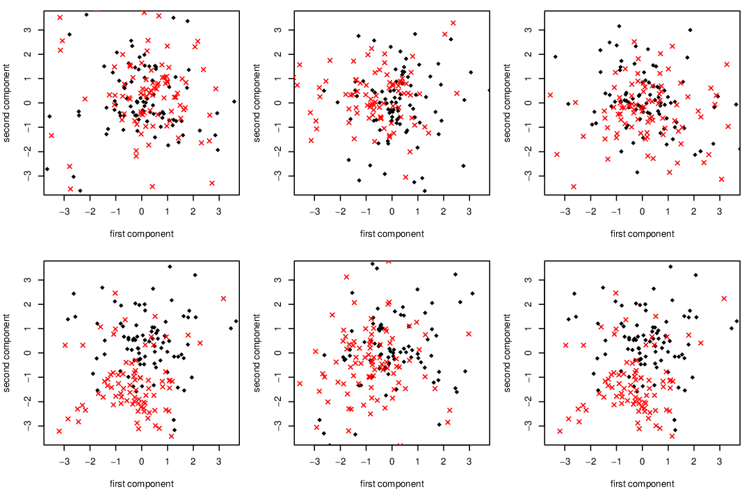
Refer to caption

Figure 1: Different two-dimensional projections of 200200 observations in p=50p=50 dimensions. Top row: three projections drawn from Haar measure; bottom row: the projected data after applying the projections with smallest estimate of test error out of 100 Haar projections with LDA (left), Quadratic Discriminant Analysis (middle) and kk-nearest neighbours (right).

One of the basic but fundamental observations that underpins our proposal is the fact that aggregating the classifications of all random projections is not always sensible, since many of these projections will typically destroy the class structure in the data; see the top row of Figure 1. For this reason, we advocate partitioning the projections into disjoint groups, and within each group we retain only the projection yielding the smallest estimate of the test error. The attraction of this strategy is illustrated in the bottom row of Figure 1, where we see a much clearer partition of the classes. Another key feature of our proposal is the realisation that a simple majority vote of the classifications based on the retained projections can be highly suboptimal; instead, we argue that the voting threshold should be chosen in a data-driven fashion in an attempt to minimise the test error of the infinite-simulation version of our random projection ensemble classifier. In fact, this estimate of the optimal threshold turns out to be remarkably effective in practice; see Section 5.2 for further details. We emphasise that our methodology can be used in conjunction with any base classifier, though we particularly have in mind classifiers designed for use in low-dimensional settings. The random projection ensemble classifier can therefore be regarded as a general technique for either extending the applicability of an existing classifier to high dimensions, or improving its performance. The methodology is implemented in an R package RPEnsemble (Cannings and Samworth, 2016).

Our theoretical results are divided into three parts. In the first, we consider a generic base classifier and a generic method for generating the random projections into ℝd\mathbb{R}^{d} and quantify the difference between the test error of the random projection ensemble classifier and its infinite-simulation counterpart as the number of projections increases. We then consider selecting random projections from non-overlapping groups by initially drawing them according to Haar measure, and then within each group retaining the projection that minimises an estimate of the test error. Under a condition implied by the widely-used sufficient dimension reduction assumption (Li, 1991; Cook, 1998; Lee et al., 2013), we can then control the difference between the test error of the random projection classifier and the Bayes risk as a function of terms that depend on the performance of the base classifier based on projected data and our method for estimating the test error, as well as a term that becomes negligible as the number of projections increases. The final part of our theory gives risk bounds for the first two of these terms for specific choices of base classifier, namely Fisher’s linear discriminant and the kk-nearest neighbour classifier. The key point here is that these bounds only depend on dd, the sample size nn and the number of projections, and not on the original data dimension pp.

The remainder of the paper is organised as follows. Our methodology and general theory are developed in Sections 2 and 3. Specific choices of base classifier as well as a general sample splitting strategy are discussed in Section 4, while Section 5 is devoted to a consideration of the practical issues of computational complexity, choice of voting threshold, projected dimension and the number of projections used. In Section 6 we present results from an extensive empirical analysis on both simulated and real data where we compare the performance of the random projection ensemble classifier with several popular techniques for high-dimensional classification. The outcomes are very encouraging, and suggest that the random projection ensemble classifier has excellent finite-sample performance in a variety of different high-dimensional classification settings. We conclude with a discussion of various extensions and open problems. Proofs are given in the Appendix and the supplementary material Cannings and Samworth (2017), which appears below the reference list.

Finally in this section, we introduce the following general notation used throughout the paper. For a sufficiently smooth real-valued function gg defined on a neighbourhood of t∈ℝt\in\mathbb{R}, let g˙​(t)\dot{g}(t) and g¨​(t)\ddot{g}(t) denote its first and second derivatives at tt, and let ⌊t⌋\lfloor t\rfloor and ⟦t⟧:=t−⌊t⌋\llbracket t\rrbracket:=t-\lfloor t\rfloor denote the integer and fractional part of tt respectively.

2 A generic random projection ensemble classifier

We start by describing our setting and defining the relevant notation. Suppose that the pair (X,Y)(X,Y) takes values in ℝp×{0,1}\mathbb{R}^{p}\times\{0,1\}, with joint distribution PP, characterised by π1:=ℙ⁡(Y=1)\pi_{1}:=\mathbb{P}(Y=1), and PrP_{r}, the conditional distribution of X|Y=rX|Y=r, for r=0,1r=0,1. For convenience, we let π0:=ℙ⁡(Y=0)=1−π1\pi_{0}:=\mathbb{P}(Y=0)=1-\pi_{1}. In the alternative characterisation of PP, we let PXP_{X} denote the marginal distribution of XX and write η⁡(x):=ℙ⁡(Y=1|X=x)\eta(x):=\mathbb{P}(Y=1|X=x) for the regression function. Recall that a classifier on ℝp\mathbb{R}^{p} is a Borel measurable function C:ℝp→{0,1}C:\mathbb{R}^{p}\rightarrow\{0,1\}, with the interpretation that we assign a point x∈ℝpx\in\mathbb{R}^{p} to class C⁡(x)C(x). We let 𝒞p\mathcal{C}_{p} denote the set of all such classifiers.

The test error of a classifier CC is11 1 We define R⁡(C)R(C) through an integral rather than R(C):=ℙ{C(X)≠Y}R(C):=\mathbb{P}\{C(X)\neq Y\} to make it clear that when CC is random (depending on training data or random projections), it should be conditioned on when computing R⁡(C)R(C).

R(C):=∫ℝp×{0,1}𝟙{C(x)≠y}dP(x,y),R(C):=\int_{\mathbb{R}^{p}\times\{0,1\}}\mathds{1}_{\{C(x)\neq y\}}\,dP(x,y),

and is minimised by the Bayes classifier

CBayes​(x):={1if η⁡(x)≥1/2;0otherwiseC^{\mathrm{Bayes}}(x):=\left\{\begin{array}[]{ll}1&\mbox{if $\eta(x)\geq 1/2$};\\ 0&\mbox{otherwise}\end{array}\right.

(e.g. Devroye, Györfi and Lugosi, 1996, p. 10). Its risk is R⁡(CBayes)=𝔼⁡[min⁡{η⁡(X),1−η⁡(X)}]R(C^{\mathrm{Bayes}})=\mathbb{E}[\min\{\eta(X),1-\eta(X)\}].

Of course, we cannot use the Bayes classifier in practice, since η\eta is unknown. Nevertheless, we often have access to a sample of training data that we can use to construct an approximation to the Bayes classifier. Throughout this section and Section 3, it is convenient to consider the training sample 𝒯n:={(x1,y1),…,(xn,yn)}\mathcal{T}_{n}:=\{(x_{1},y_{1}),\ldots,(x_{n},y_{n})\} to be fixed points in ℝp×{0,1}\mathbb{R}^{p}\times\{0,1\}. Our methodology will be applied to a base classifier Cn=Cn,𝒯n,d{C}_{n}={C}_{n,\mathcal{T}_{n,d}}, which we assume can be constructed from an arbitrary training sample 𝒯n,d\mathcal{T}_{n,d} of size nn in ℝd×{0,1}\mathbb{R}^{d}\times\{0,1\}; thus Cn{C}_{n} is a measurable function from (ℝd×{0,1})n(\mathbb{R}^{d}\times\{0,1\})^{n} to 𝒞d\mathcal{C}_{d}.

Now assume that d≤pd\leq p. We say a matrix A∈ℝd×pA\in\mathbb{R}^{d\times p} is a projection if A​AT=Id×dAA^{T}=I_{d\times d}, the dd-dimensional identity matrix. Let 𝒜=𝒜d×p:={A∈ℝd×p:A​AT=Id×d}\mathcal{A}=\mathcal{A}_{d\times p}:=\{A\in\mathbb{R}^{d\times p}:AA^{T}=I_{d\times d}\} be the set of all such matrices. Given a projection A∈𝒜A\in\mathcal{A}, define projected data ziA:=A​xiz_{i}^{A}:=Ax_{i} and yiA:=yiy_{i}^{A}:=y_{i} for i=1,…,ni=1,\ldots,n, and let 𝒯nA:={(z1A,y1A),…,(znA,ynA)}\mathcal{T}_{n}^{A}:=\{(z_{1}^{A},y_{1}^{A}),\ldots,(z_{n}^{A},y_{n}^{A})\}. The projected data base classifier corresponding to Cn{C}_{n} is CnA:(ℝd×{0,1})n→𝒞p{C}_{n}^{A}:(\mathbb{R}^{d}\times\{0,1\})^{n}\rightarrow\mathcal{C}_{p}, given by

CnA​(x)=Cn,𝒯nAA​(x):=Cn,𝒯nA​(A​x).{C}_{n}^{A}(x)={C}_{n,\mathcal{T}_{n}^{A}}^{A}(x):={C}_{n,\mathcal{T}_{n}^{A}}(Ax).

Note that although CnA{C}_{n}^{A} is a classifier on ℝp\mathbb{R}^{p}, the value of CnA​(x){C}_{n}^{A}(x) only depends on xx through its dd-dimensional projection A​xAx.

We now define a generic ensemble classifier based on random projections. For B1∈ℕB_{1}\in\mathbb{N}, let 𝐀1,…,𝐀B1\mathbf{A}_{1},\ldots,\mathbf{A}_{B_{1}} denote independent and identically distributed projections in 𝒜d×p\mathcal{A}_{d\times p}, independent of (X,Y)(X,Y). The distribution on 𝒜\mathcal{A} is left unspecified at this stage, and in fact our proposed method ultimately involves choosing this distribution depending on 𝒯n\mathcal{T}_{n}.

Now set

νn(x)=νn(B1)(x):=1B1∑b1=1B1𝟙{Cn𝐀b1(x)=1}.\nu_{n}(x)=\nu_{n}^{(B_{1})}(x):=\frac{1}{B_{1}}\sum_{b_{1}=1}^{B_{1}}\mathds{1}_{\{{C}_{n}^{\mathbf{A}_{b_{1}}}(x)=1\}}. (1)

For α∈(0,1)\alpha\in(0,1), the random projection ensemble classifier is defined to be

CnRP​(x):={1if νn​(x)≥α;0otherwise.{C}_{n}^{\mathrm{RP}}(x):=\left\{\begin{array}[]{ll}1&\mbox{if $\nu_{n}(x)\geq\alpha$;}\\ 0&\mbox{otherwise.}\end{array}\right. (2)

We emphasise again here the additional flexibility afforded by not pre-specifying the voting threshold α\alpha to be 1/21/2. Our analysis of the random projection ensemble classifier will require some further definitions. Let22 2 In order to distinguish between different sources of randomness, we will write 𝐏\mathbf{P} and 𝐄\mathbf{E} for the probability and expectation, respectively, taken over the randomness from the projections 𝐀1,…,𝐀B1\mathbf{A}_{1},\ldots,\mathbf{A}_{B_{1}}. If the training data is random, then we condition on 𝒯n\mathcal{T}_{n} when computing 𝐏\mathbf{P} and 𝐄\mathbf{E}.

μn(x):=𝐄{νn(x)}=𝐏{Cn𝐀1(x)=1}.\mu_{n}(x):=\mathbf{E}\{\nu_{n}(x)\}=\mathbf{P}\{{C}_{n}^{\mathbf{A}_{1}}(x)=1\}.

For r=0,1r=0,1, define distribution functions Gn,r:[0,1]→[0,1]G_{n,r}:[0,1]\rightarrow[0,1] by Gn,r​(t):=Pr​({x∈ℝp:μn​(x)≤t})G_{n,r}(t):=P_{r}(\{x\in\mathbb{R}^{p}:\mu_{n}(x)\leq t\}). Note that since Gn,rG_{n,r} is non-decreasing it is differentiable almost everywhere; in fact, however, the following assumption will be convenient:

Assumption 1. Gn,0G_{n,0} and Gn,1G_{n,1} are twice differentiable at α\alpha.

The first derivatives of Gn,0G_{n,0} and Gn,1G_{n,1}, when they exist, are denoted as gn,0g_{n,0} and gn,1g_{n,1} respectively; under assumption 1, these derivatives are well-defined in a neighbourhood of α\alpha. Our first main result below gives an asymptotic expansion for the expected test error 𝐄⁡{R⁡(CnRP)}\mathbf{E}\{R({C}_{n}^{\mathrm{RP}})\} of our generic random projection ensemble classifier as the number of projections increases. In particular, we show that this expected test error can be well approximated by the test error of the infinite-simulation random projection classifier

CnRP∗​(x):={1if μn​(x)≥α;0otherwise.{C}_{n}^{\mathrm{RP}^{*}}(x):=\left\{\begin{array}[]{ll}1&\mbox{if $\mu_{n}(x)\geq\alpha$;}\\ 0&\mbox{otherwise.}\end{array}\right.

Note that provided Gn,0G_{n,0} and Gn,1G_{n,1} are continuous at α\alpha, we have

R⁡(CnRP∗)=π1​Gn,1​(α)+π0​{1−Gn,0​(α)}.R({C}_{n}^{\mathrm{RP}^{*}})=\pi_{1}G_{n,1}(\alpha)+\pi_{0}\{1-G_{n,0}(\alpha)\}. (3)
Theorem 1

Assume assumption 1. Then

𝐄⁡{R⁡(CnRP)}−R⁡(CnRP∗)=γn​(α)B1+o⁡(1B1)\mathbf{E}\{R({C}_{n}^{\mathrm{RP}})\}-R({C}_{n}^{\mathrm{RP}^{*}})=\frac{\gamma_{n}(\alpha)}{B_{1}}+o\Bigl(\frac{1}{B_{1}}\Bigr)

as B1→∞B_{1}\to\infty, where

γn​(α):=(1−α−⟦B1​α⟧)​{π1​gn,1​(α)−π0​gn,0​(α)}+α⁡(1−α)2​{π1​g˙n,1​(α)−π0​g˙n,0​(α)}.\gamma_{n}(\alpha):=(1-\alpha-\llbracket B_{1}\alpha\rrbracket)\{\pi_{1}g_{n,1}(\alpha)-\pi_{0}g_{n,0}(\alpha)\}+\frac{\alpha(1-\alpha)}{2}\{\pi_{1}\dot{g}_{n,1}(\alpha)-\pi_{0}\dot{g}_{n,0}(\alpha)\}.

The proof of Theorem 1 in the Appendix is lengthy, and involves a one-term Edgeworth approximation to the distribution function of a standardised Binomial random variable. One of the technical challenges is to show that the error in this approximation holds uniformly in the binomial proportion. Related techniques can also be used to show that 𝐕𝐚𝐫⁡{R⁡(CnRP)}=O⁡(B1−1)\mathbf{Var}\{R({C}_{n}^{\mathrm{RP}})\}=O(B_{1}^{-1}) under assumption 1; see Proposition 4 in the supplementary material. Very recently, Lopes (2016) has obtained similar results to this and to Theorem 1 in the context of majority vote classification, with stronger assumptions on the relevant distributions and on the form of the voting scheme. In Figure 2, we plot the average error (plus/minus two standard deviations) of the random projection ensemble classifier in one numerical example, as we vary B1∈{2,…,500}B_{1}\in\{2,\ldots,500\}; this reveals that the Monte Carlo error stabilises rapidly, in agreement with what Lopes (2016) observed for a random forest classifier.

Refer to caption

Figure 2: The average error (black) plus/minus two standard deviations (red) over 20 sets of B1​B2B_{1}B_{2} projections for B1∈{2,…,500}B_{1}\in\{2,\ldots,500\}. We use the LDA (left), QDA (middle) and kknn (right) base classifiers. The plots show the test error for one training dataset from Model 2; the other parameters are n=50n=50, p=100p=100, d=5d=5 and B2=50B_{2}=50.

Our next result controls the test excess risk, i.e. the difference between the expected test error and the Bayes risk, of the random projection classifier in terms of the expected test excess risk of the classifier based on a single random projection. An attractive feature of this result is its generality: no assumptions are placed on the configuration of the training data 𝒯n\mathcal{T}_{n}, the distribution PP of the test point (X,Y)(X,Y) or on the distribution of the individual projections.

Theorem 2

For each B1∈ℕ∪{∞}B_{1}\in\mathbb{N}\cup\{\infty\}, we have

𝐄⁡{R⁡(CnRP)}−R⁡(CBayes)≤1min⁡(α,1−α)​[𝐄⁡{R⁡(Cn𝐀1)}−R⁡(CBayes)].\mathbf{E}\{R({C}_{n}^{\mathrm{RP}})\}-R(C^{\mathrm{Bayes}})\leq\frac{1}{\min(\alpha,1-\alpha)}\bigl[\mathbf{E}\{R({C}_{n}^{\mathbf{A}_{1}})\}-R(C^{\mathrm{Bayes}})\bigr]. (4)

When B1=∞B_{1}=\infty, we interpret R⁡(CnRP)R({C}_{n}^{\mathrm{RP}}) in Theorem 2 as R⁡(CnRP∗)R({C}_{n}^{\mathrm{RP}^{*}}). In fact, when B1=∞B_{1}=\infty and Gn,0G_{n,0} and Gn,1G_{n,1} are continuous, the bound in Theorem 2 can be improved if one is using an ‘oracle’ choice of the voting threshold α\alpha, namely

α∗∈argminα′∈[0,1]R​(Cn,α′RP∗)=argminα′∈[0,1][π1​Gn,1​(α′)+π0​{1−Gn,0​(α′)}],\alpha^{*}\in\argmin_{\alpha^{\prime}\in[0,1]}R({C}_{n,\alpha^{\prime}}^{\mathrm{RP}^{*}})=\argmin_{\alpha^{\prime}\in[0,1]}\bigl[\pi_{1}G_{n,1}(\alpha^{\prime})+\pi_{0}\{1-G_{n,0}(\alpha^{\prime})\}\bigr], (5)

where we write Cn,αRP∗{C}_{n,\alpha}^{\mathrm{RP}^{*}} to emphasise the dependence on the voting threshold α\alpha. In this case, by definition of α∗\alpha^{*} and then applying Theorem 2,

R⁡(Cn,α∗RP∗)−R⁡(CBayes)≤R⁡(Cn,1/2RP∗)−R⁡(CBayes)≤2​[𝐄⁡{R⁡(Cn𝐀1)}−R⁡(CBayes)],R({C}_{n,\alpha^{*}}^{\mathrm{RP}^{*}})-R(C^{\mathrm{Bayes}})\leq R({C}_{n,1/2}^{\mathrm{RP}^{*}})-R(C^{\mathrm{Bayes}})\leq 2\bigl[\mathbf{E}\{R({C}_{n}^{\mathbf{A}_{1}})\}-R(C^{\mathrm{Bayes}})\bigr], (6)

which improves the bound in (4) since 2≤1min⁡{α∗,(1−α∗)}2\leq\frac{1}{\min\{\alpha^{*},(1-\alpha^{*})\}}. It is also worth mentioning that if assumption 1 holds at α∗∈(0,1)\alpha^{*}\in(0,1), and Gn,0G_{n,0} and Gn,1G_{n,1} are continuous, then π1​gn,1​(α∗)=π0​gn,0​(α∗)\pi_{1}g_{n,1}(\alpha^{*})=\pi_{0}g_{n,0}(\alpha^{*}) and the constant in Theorem 1 simplifies to

γn​(α∗)=α∗​(1−α∗)2​{π1​g˙n,1​(α∗)−π0​g˙n,0​(α∗)}≥0.\gamma_{n}(\alpha^{*})=\frac{\alpha^{*}(1-\alpha^{*})}{2}\{\pi_{1}\dot{g}_{n,1}(\alpha^{*})-\pi_{0}\dot{g}_{n,0}(\alpha^{*})\}\geq 0.

3 Choosing good random projections

In this section, we study a special case of the generic random projection ensemble classifier introduced in Section 2, where we propose a screening method for choosing the random projections. Let RnA{R}_{n}^{A} be an estimator of R⁡(CnA)R({C}_{n}^{A}), based on {(z1A,y1A),…,(znA,ynA)}\{(z_{1}^{A},y_{1}^{A}),\dots,(z_{n}^{A},y_{n}^{A})\}, that takes values in the set {0,1/n,…,1}\{0,1/n,\ldots,1\}. Examples of such estimators include the training error and leave-one-out estimator; we discuss these choices in greater detail in Section 4. For B1,B2∈ℕB_{1},B_{2}\in\mathbb{N}, let {𝐀b1,b2:b1=1,…,B1,b2=1,…,B2}\{\mathbf{A}_{b_{1},b_{2}}:b_{1}=1,\ldots,B_{1},b_{2}=1,\ldots,B_{2}\} denote independent projections, independent of (X,Y)(X,Y), distributed according to Haar measure on 𝒜\mathcal{A}. One way to simulate from Haar measure on the set 𝒜\mathcal{A} is to first generate a matrix 𝐐∈ℝd×p\mathbf{Q}\in\mathbb{R}^{d\times p}, where each entry is drawn independently from a standard normal distribution, and then take 𝐀T\mathbf{A}^{T} to be the matrix of left singular vectors in the singular value decomposition of 𝐐T\mathbf{Q}^{T} (see, for example, Chikuse, 2003, Theorem 1.5.4). For b1=1,…,B1b_{1}=1,\ldots,B_{1}, let

b2∗​(b1):=sargminb2∈{1,…,B2}Rn𝐀b1,b2,b_{2}^{*}(b_{1}):=\sargmin_{b_{2}\in\{1,\dots,B_{2}\}}{R}_{n}^{\mathbf{A}_{b_{1},b_{2}}}, (7)

where sargmin\sargmin denotes the smallest index where the minimum is attained in the case of a tie. We now set 𝐀b1:=𝐀b1,b2∗​(b1)\mathbf{A}_{b_{1}}:=\mathbf{A}_{b_{1},b_{2}^{*}(b_{1})}, and consider the random projection ensemble classifier from Section 2 constructed using the independent projections 𝐀1,…,𝐀B1\mathbf{A}_{1},\ldots,\mathbf{A}_{B_{1}}.

Let

Rn∗:=minA∈𝒜⁡RnAR_{n}^{*}:=\min_{A\in\mathcal{A}}{R}_{n}^{A}

denote the optimal test error estimate over all projections. The minimum is attained here, since RnAR_{n}^{A} takes only finitely many values. We assume the following:

Assumption 2. There exists β∈(0,1]\beta\in(0,1] such that

𝐏⁡(Rn𝐀1,1≤Rn∗+|ϵn|)≥β,\mathbf{P}\bigl({R}_{n}^{\mathbf{A}_{1,1}}\leq{R}_{n}^{*}+|\epsilon_{n}|\bigr)\geq\beta,

where ϵn=ϵn(B2):=𝐄⁡{R⁡(Cn𝐀1)−Rn𝐀1}\epsilon_{n}=\epsilon_{n}^{(B_{2})}:=\mathbf{E}\{R({C}_{n}^{\mathbf{A}_{1}})-{R}_{n}^{\mathbf{A}_{1}}\}.

The quantity ϵn\epsilon_{n}, which depends on B2B_{2} because 𝐀1\mathbf{A}_{1} is selected from B2B_{2} independent random projections, can be interpreted as a measure of overfitting. Assumption 2 asks that there is a positive probability that Rn𝐀1,1R_{n}^{\mathbf{A}_{1,1}} is within |ϵn||\epsilon_{n}| of its minimum value Rn∗R_{n}^{*}. The intuition here is that spending more computational time choosing a projection by increasing B2B_{2} is potentially futile: one may find a projection with a lower error estimate, but the chosen projection will not necessarily result in a classifier with a lower test error. Under this condition, the following result controls the test excess risk of our random projection ensemble classifier in terms of the test excess risk of a classifier based on dd-dimensional data, as well as a term that reflects our ability to estimate the test error of classifiers based on projected data and a term that depends on the number of projections.

Theorem 3

Assume assumption 2. Then, for each B1,B2∈ℕB_{1},B_{2}\in\mathbb{N}, and every A∈𝒜A\in\mathcal{A},

𝐄⁡{R⁡(CnRP)}−R⁡(CBayes)≤R⁡(CnA)−R⁡(CBayes)min⁡(α,1−α)+2​|ϵn|−ϵnAmin⁡(α,1−α)+(1−β)B2min⁡(α,1−α),\mathbf{E}\{R({C}_{n}^{\mathrm{RP}})\}-R(C^{\mathrm{Bayes}})\leq\frac{R({C}_{n}^{A})-R(C^{\mathrm{Bayes}})}{\min(\alpha,1-\alpha)}+\frac{2|\epsilon_{n}|-\epsilon_{n}^{A}}{\min(\alpha,1-\alpha)}+\frac{(1-\beta)^{B_{2}}}{\min(\alpha,1-\alpha)}, (8)

where ϵnA:=R⁡(CnA)−RnA\epsilon_{n}^{A}:=R({C}_{n}^{A})-{R}_{n}^{A}.

Regarding the bound in Theorem 3 as a sum of three terms, we see that the final one can be seen as the price we have to pay for the fact that we do not have access to an infinite sample of random projections. This term can be made negligible by choosing B2B_{2} to be sufficiently large, though the value of B2B_{2} required to ensure it is below a prescribed level may depend on the training data. It should also be noted that ϵn\epsilon_{n} in the second term may increase with B2B_{2}, which reflects the fact mentioned previously that this quantity is a measure of overfitting. The behaviour of the first two terms depends on the choice of base classifier, and our aim is to show that under certain conditions, these terms can be bounded (in expectation over the training data) by expressions that do not depend on pp.

To this end, define the regression function on ℝd\mathbb{R}^{d} induced by the projection A∈𝒜A\in\mathcal{A} to be ηA​(z):=ℙ⁡(Y=1|A​X=z)\eta^{A}(z):=\mathbb{P}(Y=1|AX=z). The corresponding induced Bayes classifier, which is the optimal classifier knowing only the distribution of (A​X,Y)(AX,Y), is given by

CA−Bayes​(z):={1if ηA​(z)≥1/2;0otherwise.C^{A-\mathrm{Bayes}}(z):=\left\{\begin{array}[]{ll}1&\mbox{if $\eta^{A}(z)\geq 1/2$;}\\ 0&\mbox{otherwise.}\end{array}\right.

In order to give a condition under which there exists a projection A∈𝒜A\in\mathcal{A} for which R⁡(CnA)R({C}_{n}^{A}) is close to the Bayes risk, we will invoke an additional assumption on the form of the Bayes classifier:

Assumption 3. There exists a projection A∗∈𝒜A^{*}\in\mathcal{A} such that

PX​({x∈ℝp:η⁡(x)≥1/2}​△​{x∈ℝp:ηA∗​(A∗​x)≥1/2})=0,P_{X}(\{x\in\mathbb{R}^{p}:\eta(x)\geq 1/2\}\triangle\{x\in\mathbb{R}^{p}:\eta^{A^{*}}(A^{*}x)\geq 1/2\})=0,

where B​△​C:=(B∩Cc)∪(Bc∩C)B\triangle C:=(B\cap C^{c})\cup(B^{c}\cap C) denotes the symmetric difference of two sets BB and CC.

Assumption 3 requires that the set of points x∈ℝpx\in\mathbb{R}^{p} assigned by the Bayes classifier to class 1 can be expressed as a function of a dd-dimensional projection of xx. Note that if the Bayes decision boundary is a hyperplane, then assumption 3 holds with d=1d=1. Moreover, Proposition 1 below shows that, in fact, assumption 3 holds under the sufficient dimension reduction condition, which states that YY is conditionally independent of XX given A∗​XA^{*}X; see Cook (1998) for many statistical settings where such an assumption is natural.

Proposition 1

If YY is conditionally independent of XX given A∗​XA^{*}X, then assumption 3 holds.

The following result confirms that under assumption 3, and for a sensible choice of base classifier, we can hope for R⁡(CnA∗)R({C}_{n}^{A^{*}}) to be close to the Bayes risk.

Proposition 2

Assume assumption 3. Then R⁡(CA∗−Bayes)=R⁡(CBayes)R(C^{A^{*}-\mathrm{Bayes}})=R(C^{\mathrm{Bayes}}).

We are therefore now in a position to study the first two terms in the bound in Theorem 3 in more detail for specific choices of base classifier.

4 Possible choices of the base classifier

In this section, we change our previous perspective and regard the training data as independent random pairs with distribution PP, so our earlier statements are interpreted conditionally on 𝒯n:={(X1,Y1),…,(Xn,Yn)}\mathcal{T}_{n}:=\{(X_{1},Y_{1}),\dots,(X_{n},Y_{n})\}. For A∈𝒜A\in\mathcal{A}, we write our projected data as 𝒯nA:={(Z1A,Y1A),…,(ZnA,YnA)}\mathcal{T}_{n}^{A}:=\{(Z_{1}^{A},Y_{1}^{A}),\dots,(Z_{n}^{A},Y_{n}^{A})\}, where ZiA:=A​XiZ_{i}^{A}:=AX_{i} and YiA:=YiY_{i}^{A}:=Y_{i}. We also write ℙ\mathbb{P} and 𝔼\mathbb{E} to refer to probabilities and expectations over all random quantities. We consider particular choices of base classifier, and study the first two terms in the bound in Theorem 3.

4.1 Linear Discriminant Analysis

Linear Discriminant Analysis (LDA), introduced by Fisher (1936), is arguably the simplest classification technique. Recall that in the special case where X|Y=r∼Np​(μr,Σ)X|Y=r\sim N_{p}(\mu_{r},\Sigma), we have

sgn⁡{η⁡(x)−1/2}=sgn⁡{log⁡π1π0+(x−μ1+μ02)T​Σ−1​(μ1−μ0)},\mathrm{sgn}\{\eta(x)-1/2\}=\mathrm{sgn}\biggl\{\log\frac{\pi_{1}}{\pi_{0}}+\Bigl(x-\frac{\mu_{1}+\mu_{0}}{2}\Bigr)^{T}\Sigma^{-1}(\mu_{1}-\mu_{0})\biggr\},

so assumption 3 holds with d=1d=1 and A∗=(μ1−μ0)T​Σ−1‖Σ−1​(μ1−μ0)‖A^{*}=\frac{(\mu_{1}-\mu_{0})^{T}\Sigma^{-1}}{\|\Sigma^{-1}(\mu_{1}-\mu_{0})\|}, a 1×p1\times p matrix. In LDA, πr\pi_{r}, μr\mu_{r} and Σ\Sigma are estimated by their sample versions, using a pooled estimate of Σ\Sigma. Although LDA cannot be applied directly when p≥np\geq n since the sample covariance matrix is singular, we can still use it as the base classifier for a random projection ensemble, provided that d<nd<n. Indeed, noting that for any A∈𝒜A\in\mathcal{A}, we have A​X|Y=r∼Nd​(μrA,ΣA)AX|Y=r\sim N_{d}(\mu_{r}^{A},\Sigma^{A}), where μrA:=A​μr\mu_{r}^{A}:=A\mu_{r} and ΣA:=A​Σ​AT\Sigma^{A}:=A\Sigma A^{T}, we can define

CnA​(x)=CnA−LDA​(x):={1if log⁡π^1π^0+(A​x−μ^1A+μ^0A2)T​Ω^A​(μ^1A−μ^0A)≥0;0otherwise.{C}_{n}^{A}(x)={C}_{n}^{A-\mathrm{LDA}}(x):=\left\{\begin{array}[]{ll}1&\mbox{if $\log\frac{\hat{\pi}_{1}}{\hat{\pi}_{0}}+\bigl(Ax-\frac{\hat{\mu}_{1}^{A}+\hat{\mu}_{0}^{A}}{2}\bigr)^{T}\hat{\Omega}^{A}(\hat{\mu}^{A}_{1}-\hat{\mu}^{A}_{0})\geq 0$};\\ 0&\mbox{otherwise.}\end{array}\right. (9)

Here, π^r:=nr/n\hat{\pi}_{r}:=n_{r}/n, where nr:=∑i=1n𝟙{Yi=r}n_{r}:=\sum_{i=1}^{n}\mathds{1}_{\{Y_{i}=r\}}, μ^rA:=nr−1∑i=1nAXi𝟙{Yi=r}\hat{\mu}_{r}^{A}:=n_{r}^{-1}\sum_{i=1}^{n}AX_{i}\mathds{1}_{\{Y_{i}=r\}},

Σ^A:=1n−2∑i=1n∑r=01(AXi−μ^rA)(AXi−μ^rA)T𝟙{Yi=r}\hat{\Sigma}^{A}:=\frac{1}{n-2}\sum_{i=1}^{n}\sum_{r=0}^{1}(AX_{i}-\hat{\mu}_{r}^{A})(AX_{i}-\hat{\mu}_{r}^{A})^{T}\mathds{1}_{\{Y_{i}=r\}}

and Ω^A:=(Σ^A)−1\hat{\Omega}^{A}:=(\hat{\Sigma}^{A})^{-1}.

Write Φ\Phi for the standard normal distribution function. Under the normal model specified above, the test error of the LDA classifier can be written as

R⁡(CnA)=π0​Φ​(log⁡π^1π^0+(δ^A)T​Ω^A​(μ^¯A−μ0A)(δ^A)T​Ω^A​ΣA​Ω^A​δ^A)+π1​Φ​(log⁡π^0π^1−(δ^A)T​Ω^A​(μ^¯A−μ1A)(δ^A)T​Ω^A​ΣA​Ω^A​δ^A),\displaystyle R({C}_{n}^{A})=\pi_{0}\Phi\Biggl(\frac{\log\frac{\hat{\pi}_{1}}{\hat{\pi}_{0}}+(\hat{\delta}^{A})^{T}\hat{\Omega}^{A}(\bar{\hat{\mu}}^{A}-\mu^{A}_{0})}{\sqrt{(\hat{\delta}^{A})^{T}\hat{\Omega}^{A}\Sigma^{A}\hat{\Omega}^{A}\hat{\delta}^{A}}}\Biggr)+\pi_{1}\Phi\Biggl(\frac{\log\frac{\hat{\pi}_{0}}{\hat{\pi}_{1}}-(\hat{\delta}^{A})^{T}\hat{\Omega}^{A}(\bar{\hat{\mu}}^{A}-\mu^{A}_{1})}{\sqrt{(\hat{\delta}^{A})^{T}\hat{\Omega}^{A}\Sigma^{A}\hat{\Omega}^{A}\hat{\delta}^{A}}}\Biggr),

where δ^A:=μ^0A−μ^1A\hat{\delta}^{A}:=\hat{\mu}_{0}^{A}-\hat{\mu}_{1}^{A} and μ^¯A:=(μ^0A+μ^1A)/2\bar{\hat{\mu}}^{A}:=(\hat{\mu}_{0}^{A}+\hat{\mu}_{1}^{A})/2.

Efron (1975) studied the excess risk of the LDA classifier in an asymptotic regime in which dd is fixed as nn diverges. Specialising his results for simplicity to the case where π0=π1\pi_{0}=\pi_{1}, he showed that using the LDA classifier (9) with A=A∗A=A^{*} yields

𝔼⁡{R⁡(CnA∗)}−R⁡(CBayes)=dn​ϕ​(−Δ2)​(Δ4+1Δ)​{1+o⁡(1)}\mathbb{E}\{R({C}_{n}^{A^{*}})\}-R(C^{\mathrm{Bayes}})=\frac{d}{n}\phi\Bigl(-\frac{\Delta}{2}\Bigr)\biggl(\frac{\Delta}{4}+\frac{1}{\Delta}\biggr)\{1+o(1)\} (10)

as n→∞n\rightarrow\infty, where Δ:=∥Σ−1/2(μ0−μ1)∥=∥(ΣA∗)−1/2(μ0A∗−μ1A∗)∥\Delta:=\|\Sigma^{-1/2}(\mu_{0}-\mu_{1})\|=\|(\Sigma^{A^{*}})^{-1/2}(\mu_{0}^{A^{*}}-\mu_{1}^{A^{*}})\|.

It remains to control the errors ϵn\epsilon_{n} and ϵnA∗\epsilon_{n}^{A^{*}} in Theorem 3. For the LDA classifier, we consider the training error estimator

RnA:=1n∑i=1n𝟙{CnA−LDA(Xi)≠Yi}.{R}_{n}^{A}:=\frac{1}{n}\sum_{i=1}^{n}\mathds{1}_{\{{C}_{n}^{A-\mathrm{LDA}}(X_{i})\neq Y_{i}\}}. (11)

Devroye and Wagner (1976) provided a Vapnik–Chervonenkis bound for RnA{R}_{n}^{A} under no assumptions on the underlying data generating mechanism: for every n∈ℕn\in\mathbb{N} and ϵ>0\epsilon>0,

supA∈𝒜ℙ{|R(CnA)−RnA|>ϵ}≤8(n+1)d+1e−nϵ2/32;\sup_{A\in\mathcal{A}}\mathbb{P}\{|R({C}_{n}^{A})-{R}_{n}^{A}|>\epsilon\}\leq 8(n+1)^{d+1}e^{-n\epsilon^{2}/32}; (12)

see also Devroye et al. (1996, Theorem 23.1). We can then conclude that

𝔼​|ϵnA∗|≤𝔼​|R⁡(CnA∗)−RnA∗|\displaystyle\mathbb{E}|\epsilon_{n}^{A^{*}}|\leq\mathbb{E}\bigl|R({C}_{n}^{A^{*}})-{R}_{n}^{A^{*}}\bigr| ≤infϵ0∈(0,1)ϵ0+8(n+1)d+1∫ϵ01e−ns2/32ds\displaystyle\leq\inf_{\epsilon_{0}\in(0,1)}\epsilon_{0}+8(n+1)^{d+1}\int_{\epsilon_{0}}^{1}e^{-ns^{2}/32}\,ds
≤8​(d+1)​log⁡(n+1)+3​log⁡2+12​n.\displaystyle\leq 8\sqrt{\frac{(d+1)\log(n+1)+3\log 2+1}{2n}}. (13)

The more difficult term to deal with is

𝔼​|ϵn|=𝔼|𝐄⁡{R⁡(Cn𝐀1)−Rn𝐀1}|≤𝔼​|R⁡(Cn𝐀1)−Rn𝐀1|.\mathbb{E}|\epsilon_{n}|=\mathbb{E}\bigl|\mathbf{E}\{R({C}_{n}^{\mathbf{A}_{1}})-{R}_{n}^{\mathbf{A}_{1}}\}\bigr|\leq\mathbb{E}\bigl|R({C}_{n}^{\mathbf{A}_{1}})-{R}_{n}^{\mathbf{A}_{1}}\bigr|.

In this case, the bound (12) cannot be applied directly, because (X1,Y1),…,(Xn,Yn)(X_{1},Y_{1}),\ldots,(X_{n},Y_{n}) are no longer independent conditional on 𝐀1\mathbf{A}_{1}; indeed 𝐀1=𝐀1,b2∗​(1)\mathbf{A}_{1}=\mathbf{A}_{1,b_{2}^{*}(1)} is selected from 𝐀1,1,…,𝐀1,B2\mathbf{A}_{1,1},\ldots,\mathbf{A}_{1,B_{2}} so as to minimise an estimate of test error, which depends on the training data. Nevertheless, since 𝐀1,1,…,𝐀1,B2\mathbf{A}_{1,1},\ldots,\mathbf{A}_{1,B_{2}} are independent of 𝒯n\mathcal{T}_{n}, we still have that

ℙ{maxb2=1,…,B2|R(Cn𝐀1,b2)−Rn𝐀1,b2|>ϵ|𝐀1,1,…,𝐀1,B2}\displaystyle\mathbb{P}\Bigl\{\max_{b_{2}=1,\ldots,B_{2}}|R({C}_{n}^{\mathbf{A}_{1,b_{2}}})-{R}_{n}^{\mathbf{A}_{1,b_{2}}}|>\epsilon\Bigm|\mathbf{A}_{1,1},\ldots,\mathbf{A}_{1,B_{2}}\Bigr\} ≤∑b2=1B2ℙ⁡{|R⁡(Cn𝐀1,b2)−Rn𝐀1,b2|>ϵ|𝐀1,b2}\displaystyle\leq\sum_{b_{2}=1}^{B_{2}}\mathbb{P}\bigl\{|R({C}_{n}^{\mathbf{A}_{1,b_{2}}})-{R}_{n}^{\mathbf{A}_{1,b_{2}}}|>\epsilon\bigm|\mathbf{A}_{1,b_{2}}\bigr\}
≤8(n+1)d+1B2e−nϵ2/32.\displaystyle\leq 8(n+1)^{d+1}B_{2}e^{-n\epsilon^{2}/32}.

We can therefore conclude by almost the same argument as that leading to (13) that

𝔼​|ϵn|≤𝔼⁡{maxb2=1,…,B2⁡|R⁡(Cn𝐀1,b2)−Rn𝐀1,b2|}≤8​(d+1)​log⁡(n+1)+3​log⁡2+log⁡B2+12​n.\mathbb{E}|\epsilon_{n}|\leq\mathbb{E}\biggl\{\max_{b_{2}=1,\ldots,B_{2}}\bigl|R({C}_{n}^{\mathbf{A}_{1,b_{2}}})-{R}_{n}^{\mathbf{A}_{1,b_{2}}}\bigr|\biggr\}\leq 8\sqrt{\frac{(d+1)\log(n+1)+3\log 2+\log B_{2}+1}{2n}}. (14)

Note that none of the bounds (10), (13) and (14) depend on the original data dimension pp. Moreover, (14), together with Theorem 3, reveals a trade-off in the choice of B2B_{2} when using LDA as the base classifier. Choosing B2B_{2} to be large gives us a good chance of finding a projection with a small estimate of test error, but we may incur a small overfitting penalty as reflected by (14).

Finally, we remark that an alternative method of fitting linear classifiers is via empirical risk minimisation. In this context, Durrant and Kabán (2013, Theorem 3.1) give high probability bounds on the test error of a linear empirical risk minimisation classifier based on a single random projection, where the bounds depend on what those authors refer to as the ‘flipping probability’, namely the probability that the class assignment of a point based on the projected data differs from the assignment in the ambient space. In principle, these bounds could be combined with our Theorem 2, though the resulting expressions would depend on probabilistic bounds on flipping probabilities.

4.2 Quadratic Discriminant Analysis

Quadratic Discriminant Analysis (QDA) is designed to handle situations where the class-conditional covariance matrices are unequal. Recall that when X|Y=r∼Np​(μr,Σr)X|Y=r\sim N_{p}(\mu_{r},\Sigma_{r}), and πr=ℙ⁡(Y=r)\pi_{r}=\mathbb{P}(Y=r), for r=0,1r=0,1, the Bayes decision boundary is given by {x∈ℝp:Δ⁡(x,π0,μ0,μ1,Σ0,Σ1)=0}\{x\in\mathbb{R}^{p}:\Delta(x;\pi_{0},\mu_{0},\mu_{1},\Sigma_{0},\Sigma_{1})=0\}, where

Δ⁡(x,π0,μ0,μ1,Σ0,Σ1)\displaystyle\Delta(x;\pi_{0},\mu_{0},\mu_{1},\Sigma_{0},\Sigma_{1}) :=log⁡π1π0−12​log⁡(detΣ1detΣ0)−12​xT​(Σ1−1−Σ0−1)​x\displaystyle:=\log\frac{\pi_{1}}{\pi_{0}}-\frac{1}{2}\log\Bigl(\frac{\det\Sigma_{1}}{\det\Sigma_{0}}\Bigr)-\frac{1}{2}x^{T}(\Sigma_{1}^{-1}-\Sigma_{0}^{-1})x
+xT​(Σ1−1​μ1−Σ0−1​μ0)−12​μ1T​Σ1−1​μ1+12​μ0T​Σ0−1​μ0.\displaystyle\hskip 30.0pt+x^{T}(\Sigma_{1}^{-1}\mu_{1}-\Sigma_{0}^{-1}\mu_{0})-\frac{1}{2}\mu_{1}^{T}\Sigma_{1}^{-1}\mu_{1}+\frac{1}{2}\mu_{0}^{T}\Sigma_{0}^{-1}\mu_{0}.

In QDA, πr\pi_{r}, μr\mu_{r} and Σr\Sigma_{r} are estimated by their sample versions. If p≥min⁡(n0,n1)p\geq\min(n_{0},n_{1}), where we recall that nr:=∑i=1n𝟙{Yi=r}n_{r}:=\sum_{i=1}^{n}\mathds{1}_{\{Y_{i}=r\}}, then at least one of the sample covariance matrix estimates is singular, and QDA cannot be used directly. Nevertheless, we can still choose d<min⁡(n0,n1)d<\min(n_{0},n_{1}) and use QDA as the base classifier in a random projection ensemble. Specifically, we can set

CnA​(x)=CnA−QDA​(x):={1if Δ⁡(x,π^0,μ^0A,μ^1A,Σ^0A,Σ^1A)≥0;0otherwise,{C}_{n}^{A}(x)={C}_{n}^{A-\mathrm{QDA}}(x):=\left\{\begin{array}[]{ll}1&\mbox{if $\Delta(x;\hat{\pi}_{0},\hat{\mu}_{0}^{A},\hat{\mu}^{A}_{1},\hat{\Sigma}^{A}_{0},\hat{\Sigma}^{A}_{1})\geq 0$};\\ 0&\mbox{otherwise,}\end{array}\right.

where π^r\hat{\pi}_{r} and μ^rA\hat{\mu}_{r}^{A} were defined in Section 4.1, and where

Σ^rA:=1nr−1∑{i:YiA=r}(AXi−μ^rA)(AXi−μ^rA)T\hat{\Sigma}_{r}^{A}:=\frac{1}{n_{r}-1}\sum_{\{i:Y_{i}^{A}=r\}}(AX_{i}-\hat{\mu}_{r}^{A})(AX_{i}-\hat{\mu}_{r}^{A})^{T}

for r=0,1r=0,1. Unfortunately, analogous theory to that presented in Section 4.1 does not appear to exist for the QDA classifier; unlike for LDA, the risk does not have a closed form (note that Σ1−Σ0\Sigma_{1}-\Sigma_{0} is non-definite in general). Nevertheless, we found in our simulations presented in Section 6 that the QDA random projection ensemble classifier can perform very well in practice. In this case, we estimate the test errors using the leave-one-out method given by

RnA:=1n∑i=1n𝟙{Cn,iA(Xi)≠Yi},{R}_{n}^{A}:=\frac{1}{n}\sum_{i=1}^{n}\mathds{1}_{\{{C}_{n,i}^{A}(X_{i})\neq Y_{i}\}}, (15)

where Cn,iA{C}_{n,i}^{A} denotes the classifier CnA{C}^{A}_{n}, trained without the iith pair, i.e. based on 𝒯nA∖{ZiA,YiA}\mathcal{T}_{n}^{A}\setminus\{Z_{i}^{A},Y_{i}^{A}\}. For a method like QDA that involves estimating more parameters than LDA, we found that the leave-one-out estimator was less susceptible to overfitting than the training error estimator.

4.3 The kk-nearest neighbour classifier

The kk-nearest neighbour classifier (kknn), first proposed by Fix and Hodges (1951), is a nonparametric method that classifies the test point x∈ℝpx\in\mathbb{R}^{p} according to a majority vote over the classes of the kk nearest training data points to xx. The enormous popularity of the kknn classifier can be attributed partly due to its simplicity and intuitive appeal; however, it also has the attractive property of being universally consistent: for every fixed distribution PP, as long as k→∞k\to\infty and k/n→0k/n\to 0, the risk of the kknn classifier converges to the Bayes risk (Devroye et al., 1996, Theorem 6.4).

Hall, Park and Samworth (2008) studied the rate of convergence of the excess risk of the kk-nearest neighbour classifier under regularity conditions that require, inter alia, that pp is fixed and that the class-conditional densities have two continuous derivatives in a neighbourhood of the (p−1)(p-1)-dimensional manifold on which they cross. In such settings, the optimal choice of kk, in terms of minimising the excess risk, is O⁡(n4/(p+4))O(n^{4/(p+4)}), and the rate of convergence of the excess risk with this choice is O(n−4/(p+4))O(n^{-4/(p+4)}). Thus, in common with other nonparametric methods, there is a ‘curse of dimensionality’ effect that means the classifier typically performs poorly in high dimensions. Samworth (2012) found the optimal way of assigning decreasing weights to increasingly distant neighbours, and quantified the asymptotic improvement in risk over the unweighted version, but the rate of convergence remains the same.

We can use the kknn classifier as the base classifier for a random projection ensemble as follows: given z∈ℝdz\in\mathbb{R}^{d}, let (Z(1)A,Y(1)A),…,(Z(n)A,Y(n)A)(Z^{A}_{(1)},Y^{A}_{(1)}),\dots,(Z^{A}_{(n)},Y^{A}_{(n)}) be a re-ordering of the training data such that ‖Z(1)A−z‖≤…≤‖Z(n)A−z‖\|Z^{A}_{(1)}-z\|\leq\ldots\leq\|Z^{A}_{(n)}-z\|, with ties split at random. Now define

CnA​(x)=CnA−k​nn​(x):={1if SnA​(A​x)≥1/2;0otherwise,{C}_{n}^{A}(x)={C}_{n}^{A-k\mathrm{nn}}(x):=\left\{\begin{array}[]{ll}1&\mbox{if $S_{n}^{A}(Ax)\geq 1/2$};\\ 0&\mbox{otherwise,}\end{array}\right.

where SnA(z):=k−1∑i=1k𝟙{YA(i)=1}S_{n}^{A}(z):=k^{-1}\sum_{i=1}^{k}\mathds{1}_{\{Y^{A}_{(i)}=1\}}. The theory described in the previous paragraph can be applied to show that, under regularity conditions, 𝔼{R(CnA∗)}−R(CBayes)=O(n−4/(d+4))\mathbb{E}\{R({C}_{n}^{A^{*}})\}-R(C^{\mathrm{Bayes}})=O(n^{-4/(d+4)}).

Once again, a natural estimate of the test error in this case is the leave-one-out estimator defined in (15), where we use the same value of kk on the leave-one-out datasets as for the base classifier, and where distance ties are split in the same way as for the base classifier. For this estimator, Devroye and Wagner (1979, Theorem 4) showed that for every n∈ℕn\in\mathbb{N},

supA∈𝒜𝔼⁡[{R⁡(CnA)−RnA}2]≤1n+24​k1/2n​2​π;\sup_{A\in\mathcal{A}}\mathbb{E}[\{R({C}_{n}^{A})-{R}_{n}^{A}\}^{2}]\leq\frac{1}{n}+\frac{24k^{1/2}}{n\sqrt{2\pi}};

see also Devroye et al. (1996, Chapter 24). It follows that

𝔼​|ϵnA∗|≤(1n+24​k1/2n​2​π)1/2≤1n1/2+25/4​3​k1/4n1/2​π1/4.\mathbb{E}|\epsilon_{n}^{A^{*}}|\leq\Bigl(\frac{1}{n}+\frac{24k^{1/2}}{n\sqrt{2\pi}}\Bigr)^{1/2}\leq\frac{1}{n^{1/2}}+\frac{2^{5/4}\sqrt{3}k^{1/4}}{n^{1/2}\pi^{1/4}}.

In fact, Devroye and Wagner (1979, Theorem 1) also provided a tail bound analogous to (12) for the leave-one-out estimator: for every n∈ℕn\in\mathbb{N} and ϵ>0\epsilon>0,

supA∈𝒜ℙ{|R(CnA)−RnA|>ϵ}≤2exp(−n​ϵ218)+6exp(−n​ϵ3108​k​(3d+1))≤8exp(−n​ϵ3108​k​(3d+1)).\sup_{A\in\mathcal{A}}\mathbb{P}\{|R(C_{n}^{A})-R_{n}^{A}|>\epsilon\}\leq 2\exp\Bigl(-\frac{n\epsilon^{2}}{18}\Bigr)+6\exp\Bigl(-\frac{n\epsilon^{3}}{108k(3^{d}+1)}\Bigr)\leq 8\exp\Bigl(-\frac{n\epsilon^{3}}{108k(3^{d}+1)}\Bigr).

Arguing very similarly to Section 4.1, we can deduce that under no conditions on the data generating mechanism, and choosing ϵ0:={108​k​(3d+1)n​log⁡(8​B2)}1/3\epsilon_{0}:=\bigl\{\frac{108k(3^{d}+1)}{n}\log(8B_{2})\bigr\}^{1/3},

𝔼​|ϵn|\displaystyle\mathbb{E}|\epsilon_{n}| =∫01ℙ{maxb2=1,…,B2|R(Cn𝐀1,b2)−Rn𝐀1,b2|>ϵ}dϵ\displaystyle=\int_{0}^{1}\mathbb{P}\biggl\{\max_{b_{2}=1,\dots,B_{2}}|R(C_{n}^{\mathbf{A}_{1,b_{2}}})-R_{n}^{\mathbf{A}_{1,b_{2}}}|>\epsilon\biggr\}\,d\epsilon
≤ϵ0+8​B2​∫ϵ0∞exp⁡(−n​ϵ3108​k​(3d+1))​𝑑ϵ≤3​{4​(3d+1)}1/3​{k⁡(1+log⁡B2+3​log⁡2)n}1/3.\displaystyle\leq\epsilon_{0}+8B_{2}\int_{\epsilon_{0}}^{\infty}\exp\Bigl(-\frac{n\epsilon^{3}}{108k(3^{d}+1)}\Bigr)\,d\epsilon\leq 3\{4(3^{d}+1)\}^{1/3}\biggl\{\frac{k(1+\log B_{2}+3\log 2)}{n}\biggr\}^{1/3}.

We have therefore again bounded the expectations of the first two terms on the right-hand side of (8) by quantities that do not depend on pp.

4.4 A general strategy using sample splitting

In Sections 4.1, 4.2 and 4.3, we focused on specific choices of the base classifier to derive bounds on the expected values of the first two terms in the bound in Theorem 3. The aim of this section, on the other hand, is to provide similar guarantees that can be applied for any choice of base classifier in conjunction with a sample splitting strategy. The idea is to split the sample 𝒯n\mathcal{T}_{n} into 𝒯n,1\mathcal{T}_{n,1} and 𝒯n,2\mathcal{T}_{n,2}, say, where |𝒯n,1|=:n(1)|\mathcal{T}_{n,1}|=:n^{(1)} and |𝒯n,2|=:n(2)|\mathcal{T}_{n,2}|=:n^{(2)}. To estimate the test error of Cn(1)A{C}_{n^{(1)}}^{A}, the projected data base classifier trained on 𝒯n,1A:={(ZiA,YiA):(Xi,Yi)∈𝒯n,1}\mathcal{T}_{n,1}^{A}:=\{(Z_{i}^{A},Y_{i}^{A}):(X_{i},Y_{i})\in\mathcal{T}_{n,1}\}, we use

Rn(1),n(2)A:=1n(2)∑(Xi,Yi)∈𝒯n,2𝟙{Cn(1)A(Xi)≠Yi};{R}_{n^{(1)},n^{(2)}}^{A}:=\frac{1}{n^{(2)}}\sum_{(X_{i},Y_{i})\in\mathcal{T}_{n,2}}\mathds{1}_{\{{C}_{n^{(1)}}^{A}(X_{i})\neq Y_{i}\}};

in other words, we construct the classifier based on the projected data from 𝒯n,1\mathcal{T}_{n,1}, and count the proportion of points in 𝒯n,2\mathcal{T}_{n,2} that are misclassified. Similar to our previous approach, for the b1b_{1}th group of projections, we then select a projection 𝐀b1\mathbf{A}_{b_{1}} that minimises this estimate of test error, and construct the random projection ensemble classifier Cn(1),n(2)RPC_{n^{(1)},n^{(2)}}^{\mathrm{RP}} from

νn(1)(x):=1B1∑b1=1B1𝟙{Cn(1)𝐀b1(x)=1}.\nu_{n^{(1)}}(x):=\frac{1}{B_{1}}\sum_{b_{1}=1}^{B_{1}}\mathds{1}_{\{{C}_{n^{(1)}}^{\mathbf{A}_{b_{1}}}(x)=1\}}.

Writing Rn(1),n(2)∗:=minA∈𝒜⁡Rn(1),n(2)AR_{n^{(1)},n^{(2)}}^{*}:=\min_{A\in\mathcal{A}}R_{n^{(1)},n^{(2)}}^{A}, we introduce the following assumption analogous to assumption 2:

Assumption 2’. There exists β∈(0,1]\beta\in(0,1] such that

𝐏⁡(Rn(1),n(2)𝐀1,1≤Rn(1),n(2)∗+|ϵn(1),n(2)|)≥β,\mathbf{P}\bigl({R}_{n^{(1)},n^{(2)}}^{\mathbf{A}_{1,1}}\leq{R}_{n^{(1)},n^{(2)}}^{*}+|\epsilon_{n^{(1)},n^{(2)}}|\bigr)\geq\beta,

where ϵn(1),n(2):=𝐄⁡{R⁡(Cn(1)𝐀1)−Rn(1),n(2)𝐀1}\epsilon_{n^{(1)},n^{(2)}}:=\mathbf{E}\{R({C}_{n^{(1)}}^{\mathbf{A}_{1}})-{R}_{n^{(1)},n^{(2)}}^{\mathbf{A}_{1}}\}.

The following bound for the random projection ensemble classifier with sample splitting is then immediate from Theorem 3 and Proposition 2.

Corollary 1

Assume assumptions 2’ and 3. Then, for each B1,B2∈ℕB_{1},B_{2}\in\mathbb{N},

𝐄⁡{R⁡(Cn(1),n(2)RP)}−R⁡(CBayes)\displaystyle\mathbf{E}\{R({C}_{n^{(1)},n^{(2)}}^{\mathrm{RP}})\}-R(C^{\mathrm{Bayes}}) ≤R⁡(Cn(1)A∗)−R⁡(CA∗−Bayes)min⁡(α,1−α)+2​|ϵn(1),n(2)|−ϵn(1),n(2)A∗min⁡(α,1−α)+(1−β)B2min⁡(α,1−α),\displaystyle\leq\frac{R({C}_{n^{(1)}}^{A^{*}})-R(C^{A^{*}-\mathrm{Bayes}})}{\min(\alpha,1-\alpha)}+\frac{2|\epsilon_{n^{(1)},n^{(2)}}|-\epsilon_{n^{(1)},n^{(2)}}^{A^{*}}}{\min(\alpha,1-\alpha)}+\frac{(1-\beta)^{B_{2}}}{\min(\alpha,1-\alpha)},

where ϵn(1),n(2)A∗:=R⁡(Cn(1)A∗)−Rn(1),n(2)A∗\epsilon_{n^{(1)},n^{(2)}}^{A^{*}}:=R({C}_{n^{(1)}}^{A^{*}})-{R}_{n^{(1)},n^{(2)}}^{A^{*}}.

The main advantage of this approach is that, since 𝒯n,1\mathcal{T}_{n,1} and 𝒯n,2\mathcal{T}_{n,2} are independent, we can apply Hoeffding’s inequality to deduce that

supA∈𝒜ℙ⁡{|R⁡(Cn(1)A)−Rn(1),n(2)A|≥ϵ|𝒯n,1}≤2​e−2​n(2)​ϵ2.\sup_{A\in\mathcal{A}}\mathbb{P}\bigl\{|R({C}_{n^{(1)}}^{A})-{R}_{n^{(1)},n^{(2)}}^{A}|\geq\epsilon\bigm|\mathcal{T}_{n,1}\bigr\}\leq 2e^{-2n^{(2)}\epsilon^{2}}.

It then follows by very similar arguments to those given in Section 4.1 that

𝔼⁡(|ϵn(1),n(2)A∗||𝒯n,1)=𝔼⁡{|R⁡(Cn(1)A∗)−Rn(1),n(2)A∗||𝒯n,1}\displaystyle\mathbb{E}(|\epsilon_{n^{(1)},n^{(2)}}^{A^{*}}|\bigm|\mathcal{T}_{n,1})=\mathbb{E}\bigl\{|R({C}_{n^{(1)}}^{A^{*}})-{R}_{n^{(1)},n^{(2)}}^{A^{*}}|\bigm|\mathcal{T}_{n,1}\bigr\} ≤(1+log⁡22​n(2))1/2,\displaystyle\leq\Bigl(\frac{1+\log 2}{2n^{(2)}}\Bigr)^{1/2},
𝔼⁡(|ϵn(1),n(2)||𝒯n,1)=𝔼⁡{|R⁡(Cn(1)𝐀1)−Rn(1),n(2)𝐀1||𝒯n,1}\displaystyle\mathbb{E}(|\epsilon_{n^{(1)},n^{(2)}}|\bigm|\mathcal{T}_{n,1})=\mathbb{E}\bigl\{|R({C}_{n^{(1)}}^{\mathbf{A}_{1}})-{R}_{n^{(1)},n^{(2)}}^{\mathbf{A}_{1}}|\bigm|\mathcal{T}_{n,1}\bigr\} ≤(1+log⁡2+log⁡B22​n(2))1/2.\displaystyle\leq\Bigl(\frac{1+\log 2+\log B_{2}}{2n^{(2)}}\Bigr)^{1/2}. (16)

These bounds hold for any choice of base classifier (and still without any assumptions on the data generating mechanism); moreover, since the bounds on the terms in (16) merely rely on Hoeffding’s inequality as opposed to Vapnik–Chervonenkis theory, they are typically sharper. The disadvantage is that the first term in the bound in Corollary 1 will typically be larger than the corresponding term in Theorem 3 due to the reduced effective sample size.

5 Practical considerations

5.1 Computational complexity

The random projection ensemble classifier aggregates the results of applying a base classifier to many random projections of the data. Thus we need to compute the training error (or leave-one-out error) of the base classifier after applying each of the B1​B2B_{1}B_{2} projections. The test point is then classified using the B1B_{1} projections that yield the minimum error estimate within each block of size B2B_{2}.

Generating a random projection from Haar measure involves computing the left singular vectors of a p×dp\times d matrix, which requires O⁡(p​d2)O(pd^{2}) operations (Trefethen and Bau, 1997, Lecture 31). However, if computational cost is a concern, one may simply generate a matrix with p​dpd independent N⁡(0,1/p)N(0,1/p) entries. If pp is large, such a matrix will be approximately orthonormal with high probability. In fact, when the base classifier is affine invariant (as is the case for LDA and QDA), this will give the same results as using Haar projections, in which case one can forgo the orthonormalisation step altogether when generating the random projections. Even in very high-dimensional settings, multiplication by a random Gaussian matrix can be approximated in a computationally efficient manner (Le, Sarlos and Smola, 2013, e.g.). Once a projection is generated, we need to map the training data to the lower dimensional space, which requires O⁡(n​p​d)O(npd) operations. We then classify the training data using the base classifier. The cost of this step, denoted TtrainT_{\mathrm{train}}, depends on the choice of the base classifier; for LDA and QDA it is O⁡(n​d2)O(nd^{2}), while for kknn it is O⁡(n2​d)O(n^{2}d). Finally the test points are classified using the chosen projections; this cost, denoted TtestT_{\mathrm{test}}, also depends on the choice of base classifier. For LDA, QDA and kknn it is O⁡(ntest​d)O(n_{\mathrm{test}}d), O⁡(ntest​d2)O(n_{\mathrm{test}}d^{2}) and O⁡((n+ntest)2​d)O((n+n_{\mathrm{test}})^{2}d), respectively, where ntestn_{\mathrm{test}} is the number of test points. Overall we therefore have a cost of O⁡(B1​{B2​(n​p​d+Ttrain)+ntest​p​d+Ttest})O(B_{1}\{B_{2}(npd+T_{\mathrm{train}})+n_{\mathrm{test}}pd+T_{\mathrm{test}}\}) operations.

An appealing aspect of the proposal studied here is the scope to incorporate parallel computing. We can simultaneously compute the projected data base classifier for each of the B1​B2B_{1}B_{2} projections. In the supplementary material we present the running times of the random projection ensemble classifier and the other methods considered in the empirical comparison in Section 6.

5.2 Choice of α\alpha

We now discuss the choice of the voting threshold α\alpha. In (5), at the end of Section 2, we defined the oracle choice α∗\alpha^{*}, which minimises the test error of the infinite-simulation random projection classifier. Of course, α∗\alpha^{*} cannot be used directly, because we do not know Gn,0G_{n,0} and Gn,1G_{n,1} (and we may not know π0\pi_{0} and π1\pi_{1} either). Nevertheless, for the LDA base classifier we can estimate Gn,rG_{n,r} using

G^n,r(t):=1nr∑{i:Yi=r}𝟙{νn(Xi)<t}\hat{G}_{n,r}(t):=\frac{1}{n_{r}}\sum_{\{i:Y_{i}=r\}}\mathds{1}_{\{\nu_{n}(X_{i})<t\}}

for r=0,1r=0,1. For the QDA and kk-nearest neighbour base classifiers, we use the leave-one-out-based estimate ν~n(Xi):=B1−1∑b1=1B1𝟙{Cn,i𝐀b1(Xi)=1}\tilde{\nu}_{n}(X_{i}):=B_{1}^{-1}\sum_{b_{1}=1}^{B_{1}}\mathds{1}_{\{{C}_{n,i}^{\mathbf{A}_{b_{1}}}(X_{i})=1\}} in place of νn​(Xi)\nu_{n}(X_{i}). We also estimate πr\pi_{r} by π^r:=n−1∑i=1n𝟙{Yi=r}\hat{\pi}_{r}:=n^{-1}\sum_{i=1}^{n}\mathds{1}_{\{Y_{i}=r\}}, and then set the cut-off in (2) as

α^∈argminα′∈[0,1][π^1​G^n,1​(α′)+π^0​{1−G^n,0​(α′)}].\hat{\alpha}\in\argmin_{\alpha^{\prime}\in[0,1]}\bigl[\hat{\pi}_{1}\hat{G}_{n,1}(\alpha^{\prime})+\hat{\pi}_{0}\{1-\hat{G}_{n,0}(\alpha^{\prime})\}\bigr]. (17)

Since empirical distribution functions are piecewise constant, the objective function in (17) does not have a unique minimum, so we choose α^\hat{\alpha} to be the average of the smallest and largest minimisers. An attractive feature of the method is that {νn(Xi):i=1,…,n}\{\nu_{n}(X_{i}):i=1,\ldots,n\} (or {ν~n(Xi):i=1,…,n}\{\tilde{\nu}_{n}(X_{i}):i=1,\ldots,n\} in the case of QDA and kknn) are already calculated in order to choose the projections, so calculating G^n,0\hat{G}_{n,0} and G^n,1\hat{G}_{n,1} carries negligible extra computational cost.

Figure 3 illustrates π^1​G^n,1​(α′)+π^0​{1−G^n,0​(α′)}\hat{\pi}_{1}\hat{G}_{n,1}(\alpha^{\prime})+\hat{\pi}_{0}\{1-\hat{G}_{n,0}(\alpha^{\prime})\} as an estimator of π1​Gn,1​(α′)+π0​{1−Gn,0​(α′)}\pi_{1}G_{n,1}(\alpha^{\prime})+\pi_{0}\{1-G_{n,0}(\alpha^{\prime})\}, for the QDA base classifier and for different values of nn and π1\pi_{1}. Here, a very good approximation to the estimand was obtained using an independent data set of size 5000. Unsurprisingly, the performance of the estimator improves as nn increases, but the most notable feature of these plots is the fact that for all classifiers and even for small sample sizes, α^\hat{\alpha} is an excellent estimator of α∗\alpha^{*}, and may be a substantial improvement on the naive choice α^=1/2\hat{\alpha}=1/2 (or the appropriate prior weighted choice), which may result in a classifier that assigns every point to a single class.

Refer to caption

Figure 3: π1​Gn,1​(α′)+π0​{1−Gn,0​(α′)}\pi_{1}G_{n,1}(\alpha^{\prime})+\pi_{0}\{1-G_{n,0}(\alpha^{\prime})\} in (5) (black) and π^1​G^n,1​(α′)+π^0​{1−G^n,0​(α′)}\hat{\pi}_{1}\hat{G}_{n,1}(\alpha^{\prime})+\hat{\pi}_{0}\{1-\hat{G}_{n,0}(\alpha^{\prime})\} (red) for the QDA base classifier after projecting for one training data set of size n=50n=50 (left), 200200 (middle) and 10001000 (right) from Model 3 with π1=0.5\pi_{1}=0.5 (top) and π1=0.66\pi_{1}=0.66 (bottom). Here, p=100p=100 and d=2d=2.

5.3 Choice of B1B_{1} and B2B_{2}

In order to minimise the Monte Carlo error as described in Theorem 1 and Proposition 4, we should choose B1B_{1} to be as large as possible. The constraint, of course, is that the computational cost of the random projection classifier scales linearly with B1B_{1}. The choice of B2B_{2} is more subtle; while the third term in the bound in Theorem 3 decreases as B2B_{2} increases, we saw in Section 4 that upper bounds on 𝔼​|ϵn|\mathbb{E}|\epsilon_{n}| may increase with B2B_{2}. In principle, we could try to use the expressions given in Theorem 3 and Section 4 to choose B2B_{2} to minimise the overall upper bound on 𝐄⁡{R⁡(CnRP)}−R⁡(CBayes)\mathbf{E}\{R({C}_{n}^{\mathrm{RP}})\}-R(C^{\mathrm{Bayes}}). In practice, however, we found that an involved approach such as this was unnecessary, and that the ensemble method was robust to the choice of B1B_{1} and B2B_{2}; see Section 11 of the supplementary material for numerical evidence and further discussion. Based on this numerical work, we recommend B1=500B_{1}=500 and B2=50B_{2}=50 as sensible default choices, and indeed these values were used in all of our experiments in Section 6 as well as Section 12 in the supplementary material.

5.4 Choice of dd

We want to choose dd as small as possible in order to obtain the best possible performance bounds as described in Section 4 above. This also reduces the computational cost. However, the performance bounds rely on assumption 3, whose strength decreases as dd increases, so we want to choose dd large enough that this condition holds (at least approximately).

In Section 6 we see that the random projection ensemble method is quite robust to the choice of dd. Nevertheless, in some circumstances it may be desirable to have an automatic choice, and cross-validation provides one possible approach when computational cost at training time is not too constrained. Thus, if we wish to choose dd from a set 𝒟⊆{1,…,p}\mathcal{D}\subseteq\{1,\dots,p\}, then for each d∈𝒟d\in\mathcal{D}, we train the random projection ensemble classifier, and set

d^:=sargmind∈𝒟[π^1​G^n,1​(α^)+π^0​{1−G^n,0​(α^)}],\hat{d}:=\sargmin_{d\in\mathcal{D}}\bigl[\hat{\pi}_{1}\hat{G}_{n,1}(\hat{\alpha})+\hat{\pi}_{0}\{1-\hat{G}_{n,0}(\hat{\alpha})\}\bigr],

where α^=α^d\hat{\alpha}=\hat{\alpha}_{d} is given in (17). Such a proceedure does not add to the computational cost at test time. This strategy is most appropriate when max⁡{d:d∈𝒟}\max\{d:d\in\mathcal{D}\} is not too large (which is the setting we have in mind); otherwise a penalised risk approach may be more suitable.

6 Empirical analysis

In this section, we assess the empirical performance of the random projection ensemble classifier in simulated and real data experiments. We will write RP-LDAd, RP-QDAd and RP-kknnd to denote the random projection classifier with LDA, QDA, and kknn base classifiers, respectively; the subscript dd refers to the dimension of the image space of the projections.

For comparison we present the corresponding results of applying, where possible, the three base classifiers (LDA, QDA, kknn) in the original pp-dimensional space alongside 11 other classification methods chosen to represent the state of the art. These include Random Forests (RF) (Breiman, 2001); Support Vector Machines (SVM) (Cortes and Vapnik, 1995); Gaussian Process (GP) classifiers (Williams and Barber, 1998); and three methods designed for high-dimensional classification problems, namely Penalized LDA (PenLDA) (Witten and Tibshirani, 2011), Nearest Shrunken Centroids (NSC) (Tibshirani et al., 2003), and ℓ1\ell_{1}-penalised logistic regression (PenLog) (Goeman et al., 2015).

A further comparison is with LDA and kknn applied after a single projection chosen based on the sufficient dimension reduction assumption (SDR5). For this method, we project the data into 5 dimensions using the proposal of Shin et al. (2014). This method requires n>pn>p. Finally, we compare with two related ensemble methods: optimal tree ensembles (OTE) (Khan et al., 2015a) and ensemble of subset of kk-nearest neighbour classifiers (ESkknn) (Gul et al., 2016).

Many of these methods require tuning parameter selection, and the parameters were chosen as follows: for the standard kknn classifier, we chose kk via leave-one-out cross validation from the set {3,5,7,9,11}\{3,5,7,9,11\}. The Random Forest was implemented using the randomForest package (Liaw and Wiener, 2014); we used an ensemble of 1000 trees, with ⌊p⌋\lfloor\sqrt{p}\rfloor (the default setting in the randomForest package) components randomly selected when training each tree. For the Radial SVM, we used the reproducing basis kernel K⁡(u,v):=exp⁡(−1p​‖u−v‖2)K(u,v):=\exp(-\frac{1}{p}\|u-v\|^{2}). Both SVM classifiers were implemented using the svm function in the e1071 package (Meyer et al., 2015). The GP classifier uses a radial basis function, with the hyperparameter chosen via the automatic method in the gausspr function in the kernlab package (Karatzoglou, Smola and Hornik, 2015). The tuning parameters for the other methods were chosen using the default settings in the corresponding R packages PenLDA (Witten, 2011), NSC (Hastie et al., 2015) and penalized (Goeman et al., 2015) namely 6-fold, 10-fold and 5-fold cross validation, respectively. For the OTE and ESkknn methods we used the default settings in the R packages OTE (Khan et al., 2015b) and ESKNN (Gul et al., 2015).

6.1 Simulated examples

We present four different simulation settings chosen to investigate the performance of the random projection ensemble classifier in a wide variety of scenarios. In each of the examples below, we take n∈{50,200,1000}n\in\{50,200,1000\}, p∈{100,1000}p\in\{100,1000\} and investigate two different values of the prior probability. We use Gaussian projections (cf. Section 5.1) and set B1=500B_{1}=500 and B2=50B_{2}=50 (cf. Section 5.3).

The risk estimates and standard errors for the p=100p=100 and π1=0.5\pi_{1}=0.5 case are shown in Tables 1 and 2 (the remaining results are given in the supplementary material). These were calculated as follows: We set ntest=1000n_{\mathrm{test}}=1000, Nreps=100N_{\mathrm{reps}}=100, and for l=1,…,Nrepsl=1,\ldots,N_{\mathrm{reps}} we generate a training set of size nn and a test set of size ntestn_{\mathrm{test}} from the same distribution. Let R^l\hat{R}_{l} be the proportion of the test set that is classified incorrectly in the llth repeat of the experiment. The overall risk estimate presented is Risk^:=1Nreps​∑l=1NrepsR^l\widehat{\mathrm{Risk}}:=\frac{1}{N_{\mathrm{reps}}}\sum_{l=1}^{N_{\mathrm{reps}}}\hat{R}_{l}. Note that

𝔼⁡{Risk^}=𝔼⁡{R⁡(CnRP)}\mathbb{E}\{\widehat{\mathrm{Risk}}\}=\mathbb{E}\{R({C}_{n}^{\mathrm{RP}})\}

and

Var⁡(Risk^)\displaystyle\mathrm{Var}(\widehat{\mathrm{Risk}}) =1Nreps​Var​(R^1)\displaystyle=\frac{1}{N_{\mathrm{reps}}}\mathrm{Var}(\hat{R}_{1})
=1Nreps​[𝔼⁡{𝐄​{R⁡(CnRP)}​[1−𝐄⁡{R⁡(CnRP)}]ntest}+Var⁡[𝐄⁡{R⁡(CnRP)}]].\displaystyle=\frac{1}{N_{\mathrm{reps}}}\biggl[\mathbb{E}\biggl\{\frac{\mathbf{E}\{R({C}_{n}^{\mathrm{RP}})\}[1-\mathbf{E}\{R({C}_{n}^{\mathrm{RP}})\}]}{n_{\mathrm{test}}}\biggr\}+\mathrm{Var}\bigl[\mathbf{E}\{R({C}_{n}^{\mathrm{RP}})\}\bigr]\biggr].

We therefore estimate the standard error in the tables below by

σ^:=1Nreps1/2​{Risk^​(1−Risk^)ntest+ntest−1ntest​Nreps​∑l=1Nreps(R^l−Risk^)2}1/2.\hat{\sigma}:=\frac{1}{N_{\mathrm{reps}}^{1/2}}\biggl\{\frac{\widehat{\mathrm{Risk}}(1-\widehat{\mathrm{Risk}})}{n_{\mathrm{test}}}+\frac{n_{\mathrm{test}}-1}{n_{\mathrm{test}}N_{\mathrm{reps}}}\sum_{l=1}^{N_{\mathrm{reps}}}(\hat{R}_{l}-\widehat{\mathrm{Risk}})^{2}\biggr\}^{1/2}.

The method with the smallest risk estimate in each column of the tables below is highlighted in bold; where applicable, we also highlight any method with a risk estimate within one standard error of the minimum.

6.1.1 Sparse class boundaries

Model 1: Here, X|{Y=0}∼12Np(μ0,Σ)+12Np(−μ0,Σ)X|\{Y=0\}\sim\frac{1}{2}N_{p}(\mu_{0},\Sigma)+\frac{1}{2}N_{p}(-\mu_{0},\Sigma), and X|{Y=1}∼12Np(μ1,Σ)+12Np(−μ1,Σ)X|\{Y=1\}\sim\frac{1}{2}N_{p}(\mu_{1},\Sigma)+\frac{1}{2}N_{p}(-\mu_{1},\Sigma), where, for p=100p=100, we set Σ=I100×100\Sigma=I_{100\times 100}, μ0=(2,−2,0,…,0)T\mu_{0}=(2,-2,0,\ldots,0)^{T} and μ1=(2,2,0,…,0)T\mu_{1}=(2,2,0,\ldots,0)^{T}.

In Model 1, assumption 3 holds with d=2d=2; for example, we could take the rows of A∗A^{*} to be the first two Euclidean basis vectors. We see that the RP ensemble classifier with the QDA base classifier performs very well here, as does the OTE method. Despite the fact that the regression function η\eta only depends on the first two components in this example, the comparators designed for sparse problems do not perform well; in some cases they are no better than a random guess.

6.1.2 Rotated Sparse Normal

Model 2: Here, X|{Y=0}∼Np(Ωpμ0,ΩpΣ0ΩpT)X|\{Y=0\}\sim N_{p}(\Omega_{p}\mu_{0},\Omega_{p}\Sigma_{0}\Omega_{p}^{T}), and X|{Y=1}∼Np(Ωpμ1,ΩpΣ1ΩpT)X|\{Y=1\}\sim N_{p}(\Omega_{p}\mu_{1},\Omega_{p}\Sigma_{1}\Omega_{p}^{T}), where Ωp\Omega_{p} is a p×pp\times p rotation matrix that was sampled once according to Haar measure, and remained fixed thereafter, and we set μ0=(3,3,3,0,…,0)T\mu_{0}=(3,3,3,0,\dots,0)^{T} and μ1=(0,…,0)T\mu_{1}=(0,\ldots,0)^{T}. Moreover, Σ0\Sigma_{0} and Σ1\Sigma_{1} are block diagonal, with blocks Σr(1)\Sigma_{r}^{(1)}, and Σr(2)\Sigma_{r}^{(2)}, for r=0,1r=0,1, where Σ0(1)\Sigma_{0}^{(1)} is a 3×33\times 3 matrix with diagonal entries equal to 2 and off-diagonal entries equal to 1/2, and Σ1(1)=Σ0(1)−I3×3\Sigma_{1}^{(1)}=\Sigma_{0}^{(1)}-I_{3\times 3}. In both classes Σr(2)\Sigma_{r}^{(2)} is a (p−3)×(p−3)(p-3)\times(p-3) matrix, with diagonal entries equal to 1 and off-diagonal entries equal to 1/2.

In Model 2, assumption 3 holds with d=3d=3; for instance, A∗A^{*} can be taken to be the first three rows of ΩpT\Omega_{p}^{T}. Perhaps surprisingly, whether we use too small a value of dd (namely d=2d=2), or one that is too large (d=5d=5), the RP ensemble methods still classify very well.

Table 1: Misclassification rates for Models 1 and 2, with p=100p=100 and π1=0.5\pi_{1}=0.5.

Model 1, Bayes risk = 4.45 Model 2, Bayes risk = 4.09 nn 5050 200200 10001000 5050 200200 10001000 RP-LDA2 49.340.2649.34_{0.26} 48.100.3148.10_{0.31} 44.140.4644.14_{0.46} 8.340.288.34_{0.28} 5.560.12\mathbf{5.56}_{0.12} 5.170.10\mathbf{5.17}_{0.10} RP-LDA5 49.810.2449.81_{0.24} 48.860.3048.86_{0.30} 46.910.4046.91_{0.40} 8.170.27\mathbf{8.17}_{0.27} 5.640.13\mathbf{5.64}_{0.13} 5.140.10\mathbf{5.14}_{0.10} RP-QDA2 44.180.2944.18_{0.29} 29.380.4929.38_{0.49} 10.570.2210.57_{0.22} 8.400.298.40_{0.29} 5.570.12\mathbf{5.57}_{0.12} 5.160.10\mathbf{5.16}_{0.10} RP-QDA5 39.320.3339.32_{0.33} 22.320.32\mathbf{22.32}_{0.32} 8.750.15\mathbf{8.75}_{0.15} 8.060.25\mathbf{8.06}_{0.25} 5.580.12\mathbf{5.58}_{0.12} 5.090.10\mathbf{5.09}_{0.10} RP-kknn2 46.100.3046.10_{0.30} 36.180.3236.18_{0.32} 19.420.2019.42_{0.20} 8.940.368.94_{0.36} 5.600.12\mathbf{5.60}_{0.12} 5.200.105.20_{0.10} RP-kknn5 43.650.3043.65_{0.30} 25.340.3525.34_{0.35} 10.210.1610.21_{0.16} 9.000.339.00_{0.33} 5.680.12\mathbf{5.68}_{0.12} 5.130.10\mathbf{5.13}_{0.10} LDA N/A 49.600.2349.60_{0.23} 49.910.2249.91_{0.22} N/A 14.320.2214.32_{0.22} 6.340.116.34_{0.11} QDA N/A N/A 27.360.2327.36_{0.23} N/A N/A 17.100.2017.10_{0.20} kknn 34.660.35\mathbf{34.66}_{0.35} 23.710.3123.71_{0.31} 15.310.1715.31_{0.17} 12.810.2812.81_{0.28} 8.800.158.80_{0.15} 7.280.137.28_{0.13} RF 49.720.2349.72_{0.23} 48.330.2548.33_{0.25} 43.280.4343.28_{0.43} 11.110.3111.11_{0.31} 6.800.126.80_{0.12} 6.070.116.07_{0.11} Radial SVM 49.830.2249.83_{0.22} 50.160.2250.16_{0.22} 48.670.2248.67_{0.22} 24.041.4724.04_{1.47} 6.370.146.37_{0.14} 5.460.105.46_{0.10} Linear SVM 50.020.2350.02_{0.23} 49.550.2149.55_{0.21} 50.040.2250.04_{0.22} 9.410.219.41_{0.21} 8.960.178.96_{0.17} 7.760.137.76_{0.13} Radial GP 48.180.3048.18_{0.30} 42.760.2942.76_{0.29} 26.600.2426.60_{0.24} 14.090.6314.09_{0.63} 5.840.135.84_{0.13} 5.090.10\mathbf{5.09}_{0.10} PenLDA 49.950.2349.95_{0.23} 49.790.2349.79_{0.23} 50.050.2250.05_{0.22} 11.110.5511.11_{0.55} 6.720.206.72_{0.20} 5.790.125.79_{0.12} NSC 49.740.2349.74_{0.23} 49.690.2649.69_{0.26} 49.550.2449.55_{0.24} 12.610.6112.61_{0.61} 7.270.287.27_{0.28} 5.820.135.82_{0.13} PenLog 49.660.3549.66_{0.35} 49.880.2449.88_{0.24} 50.120.2150.12_{0.21} 11.370.2211.37_{0.22} 7.670.147.67_{0.14} 6.000.116.00_{0.11} SDR5-LDA N/A 37.800.4837.80_{0.48} 35.310.3035.31_{0.30} N/A 15.070.2215.07_{0.22} 6.470.116.47_{0.11} SDR5-kknn N/A 32.220.7132.22_{0.71} 21.831.0821.83_{1.08} N/A 18.810.2918.81_{0.29} 7.750.127.75_{0.12} OTE 48.510.3348.51_{0.33} 34.731.2334.73_{1.23} 9.570.669.57_{0.66} 18.260.4718.26_{0.47} 12.440.2612.44_{0.26} 9.240.159.24_{0.15} ESkknn 50.130.2350.13_{0.23} 49.870.2249.87_{0.22} 49.770.2149.77_{0.21} 40.300.7140.30_{0.71} 37.060.6337.06_{0.63} 32.980.5832.98_{0.58}

6.1.3 Independent features

Model 3: Here, P0=Np​(μ,Ip×p)P_{0}=N_{p}(\mu,I_{p\times p}), with μ=1p​(1,…,1,0,…,0)T\mu=\frac{1}{\sqrt{p}}(1,\dots,1,0,\ldots,0)^{T}, where μ\mu has p/2p/2 non-zero components, while P1P_{1} is the distribution of pp independent components, each with a standard Laplace distribution.

In Model 3, the class boundaries are non-linear and, in fact, assumption 3 is not satisfied for any d<pd<p. Nevertheless, in Table 2, we see that where the LDA, QDA and kknn classifiers are tractable, they are outperformed by their random projection ensemble counterparts, and in fact the RP-QDA5 classifier has the smallest misclassification rate among all methods implemented. Unsurprisingly, the methods that are designed for a linear Bayes decision boundary are not effective. The RP-QDA classifiers are especially accurate here; in particular, they are able to cope better with the non-linearity of the class boundaries than the RP-LDA classifiers.

6.1.4 tt-distributed features

Model 4: Here, X|{Y=r}=μr+ZrUr/νrX|\{Y=r\}=\mu_{r}+\frac{Z_{r}}{\sqrt{U_{r}/\nu_{r}}}, where Zr∼Np​(0,Σr)Z_{r}\sim N_{p}(0,\Sigma_{r}) independent of Ur∼χνr2U_{r}\sim\chi^{2}_{\nu_{r}}, for r=0,1r=0,1. That is, PrP_{r} is the multivariate tt-distribution centred at μr\mu_{r}, with νr\nu_{r} degrees of freedom and shape parameter Σr\Sigma_{r}. We set μ0=(1,…,1,0,…,0)T\mu_{0}=(1,\dots,1,0,\dots,0)^{T}, where μ0\mu_{0} has 10 non-zero components, μ1=0\mu_{1}=0, ν0=2\nu_{0}=2, ν1=1\nu_{1}=1, Σ0=(Σj,k)\Sigma_{0}=(\Sigma_{j,k}), where Σj,j=1\Sigma_{j,j}=1, Σj,k=0.5\Sigma_{j,k}=0.5 if max⁡(j,k)≤10\max(j,k)\leq 10 and j≠kj\neq k, Σj,k=0\Sigma_{j,k}=0 otherwise, and Σ1=Ip×p\Sigma_{1}=I_{p\times p}.

Table 2: Misclassification rates for Models 3 and 4, with p=100p=100 and π1=0.5\pi_{1}=0.5.

Model 3, Bayes risk = 1.01 Model 4, Bayes risk = 12.68 nn 5050 200200 10001000 5050 200200 10001000 RP-LDA2 45.111.0345.11_{1.03} 44.050.9844.05_{0.98} 39.220.8939.22_{0.89} 38.060.7138.06_{0.71} 38.450.9238.45_{0.92} 40.480.8440.48_{0.84} RP-LDA5 45.580.6045.58_{0.60} 44.460.5844.46_{0.58} 41.080.5641.08_{0.56} 34.840.6334.84_{0.63} 32.430.7532.43_{0.75} 35.090.8935.09_{0.89} RP-QDA2 11.410.6211.41_{0.62} 4.830.154.83_{0.15} 3.850.093.85_{0.09} 42.120.4742.12_{0.47} 41.990.2841.99_{0.28} 42.370.2142.37_{0.21} RP-QDA5 9.710.52\mathbf{9.71}_{0.52} 4.230.14\mathbf{4.23}_{0.14} 3.290.08\mathbf{3.29}_{0.08} 42.130.3542.13_{0.35} 42.040.2742.04_{0.27} 42.590.2142.59_{0.21} RP-kknn2 20.690.8420.69_{0.84} 6.860.276.86_{0.27} 4.730.114.73_{0.11} 30.850.4930.85_{0.49} 24.070.3124.07_{0.31} 20.760.1920.76_{0.19} RP-kknn5 21.300.5421.30_{0.54} 6.910.186.91_{0.18} 3.780.103.78_{0.10} 29.850.46\mathbf{29.85}_{0.46} 24.020.3024.02_{0.30} 20.810.2120.81_{0.21} LDA N/A 46.220.2546.22_{0.25} 41.740.2441.74_{0.24} N/A 37.340.2937.34_{0.29} 31.040.2631.04_{0.26} QDA N/A N/A 15.300.2115.30_{0.21} N/A N/A 40.900.2140.90_{0.21} kknn 49.920.2449.92_{0.24} 49.810.2249.81_{0.22} 49.670.2249.67_{0.22} 37.490.6337.49_{0.63} 30.140.3430.14_{0.34} 27.580.2527.58_{0.25} RF 44.790.3444.79_{0.34} 23.380.3023.38_{0.30} 7.720.167.72_{0.16} 30.970.6030.97_{0.60} 20.460.21\mathbf{20.46}_{0.21} 18.690.17\mathbf{18.69}_{0.17} Radial SVM 39.341.4739.34_{1.47} 4.650.134.65_{0.13} 3.430.093.43_{0.09} 47.720.4047.72_{0.40} 45.460.5145.46_{0.51} 43.700.7243.70_{0.72} Linear SVM 46.570.2646.57_{0.26} 46.170.2446.17_{0.24} 41.670.2641.67_{0.26} 36.790.5736.79_{0.57} 34.210.5634.21_{0.56} 31.870.7131.87_{0.71} Radial GP 48.870.3148.87_{0.31} 45.470.3745.47_{0.37} 36.180.2736.18_{0.27} 38.390.8438.39_{0.84} 26.630.4426.63_{0.44} 22.770.2022.77_{0.20} PenLDA 46.040.2646.04_{0.26} 44.480.2644.48_{0.26} 41.710.2341.71_{0.23} 45.640.4445.64_{0.44} 45.220.5345.22_{0.53} 45.390.4745.39_{0.47} NSC 47.470.3347.47_{0.33} 45.990.3445.99_{0.34} 42.310.3042.31_{0.30} 46.340.5846.34_{0.58} 44.690.6944.69_{0.69} 45.720.6545.72_{0.65} PenLog 48.810.2948.81_{0.29} 46.360.2846.36_{0.28} 42.150.2442.15_{0.24} N/A N/A N/A SDR5-LDA N/A 46.270.2446.27_{0.24} 42.090.2542.09_{0.25} N/A 37.960.2937.96_{0.29} 31.040.2731.04_{0.27} SDR5-kknn N/A 46.140.2746.14_{0.27} 36.280.2436.28_{0.24} N/A 39.700.3239.70_{0.32} 29.310.2629.31_{0.26} OTE 46.740.2846.74_{0.28} 30.620.3330.62_{0.33} 11.430.1911.43_{0.19} 32.240.5132.24_{0.51} 23.370.2823.37_{0.28} 19.590.1919.59_{0.19} ESkknn 48.660.2648.66_{0.26} 46.590.2646.59_{0.26} 45.170.2245.17_{0.22} 46.150.5146.15_{0.51} 44.030.5444.03_{0.54} 43.770.4643.77_{0.46}

Model 4 explores the effect of heavy tails and the presence of correlation between the features. Again, assumption 3 is not satisfied for any d<pd<p. The RF, OTE and RP-kknn methods all perform very well here. The RP-LDA and RP-QDA classifiers are less good. This is partly due the fact that the class-conditional distributions do not have finite second and first moments, respectively, and, as a result, the class mean and covariance matrix estimates are poor.

6.2 Real data examples

In this section, we compare the classifiers above on eight real datasets available from the UC Irvine (UCI) Machine Learning Repository. In each example, we first subsample the data to form a training set of size nn, then use the remaining data (or, where available, take a subsample of size 1000 from it) to form the test set. As with the simulated examples, we set B1=500B_{1}=500, B2=50B_{2}=50, used Gaussian distributed projections, and each experiment was repeated 100 times. Where appropriate, the tuning parameters were chosen via the methods described at the beginning of Section 6 for each of the 100 repeats of the experiment.

6.2.1 Eye state detection

The electroencephalogram eye state dataset (http://archive.ics.uci.edu/ml/datasets/EEG+Eye+State) consists of p=14p=14 EEG measurements on 14980 observations. The task is to use the EEG reading to determine the state of the eye. There are 8256 observations for which the eye is open (class 0), and 6723 for which the eye is closed (class 1).

6.2.2 Ionosphere dataset

The Ionosphere dataset (http://archive.ics.uci.edu/ml/datasets/Ionosphere) consists of p=32p=32 high-frequency antenna measurements on 351 observations. Observations are classified as good (class 0) or bad (class 1), depending on whether there is evidence for free electrons in the Ionosphere or not. The class sizes are 225 (good) and 126 (bad).

Table 3: Misclassification rates for the Eye State and Ionosphere datasets

Eye State Ionosphere nn 5050 200200 10001000 5050 100100 200200 RP-LDA5 42.060.3842.06_{0.38} 38.610.2938.61_{0.29} 36.300.2136.30_{0.21} 13.050.3813.05_{0.38} 10.750.2510.75_{0.25} 9.780.269.78_{0.26} RP-QDA5 38.970.39\mathbf{38.97}_{0.39} 32.440.4232.44_{0.42} 30.910.8730.91_{0.87} 8.140.37\mathbf{8.14}_{0.37} 6.150.22\mathbf{6.15}_{0.22} 5.210.20\mathbf{5.21}_{0.20} RP-kknn5 39.370.39\mathbf{39.37}_{0.39} 26.910.27\mathbf{26.91}_{0.27} 13.540.19\mathbf{13.54}_{0.19} 13.050.4613.05_{0.46} 7.430.257.43_{0.25} 5.430.195.43_{0.19} LDA 42.380.4042.38_{0.40} 39.150.3039.15_{0.30} 36.910.2336.91_{0.23} 23.720.4023.72_{0.40} 18.270.2818.27_{0.28} 15.580.3115.58_{0.31} QDA 39.910.3539.91_{0.35} 29.240.4029.24_{0.40} 29.761.0729.76_{1.07} N/A N/A 14.070.3414.07_{0.34} kknn 41.700.4041.70_{0.40} 29.180.2729.18_{0.27} 14.450.1614.45_{0.16} 21.810.7321.81_{0.73} 18.050.4618.05_{0.46} 16.400.3516.40_{0.35} RF 39.270.37\mathbf{39.27}_{0.37} 29.040.2529.04_{0.25} 17.630.2017.63_{0.20} 10.520.3010.52_{0.30} 7.540.197.54_{0.19} 6.480.186.48_{0.18} Radial SVM 46.330.4946.33_{0.49} 38.710.4638.71_{0.46} 31.030.6831.03_{0.68} 27.671.1527.67_{1.15} 12.850.9112.85_{0.91} 6.670.226.67_{0.22} Linear SVM 42.380.4242.38_{0.42} 39.550.3639.55_{0.36} 38.580.3838.58_{0.38} 19.410.3519.41_{0.35} 17.050.2717.05_{0.27} 15.480.2915.48_{0.29} Radial GP 40.730.3840.73_{0.38} 32.220.2532.22_{0.25} 21.660.2121.66_{0.21} 22.290.7222.29_{0.72} 17.810.4617.81_{0.46} 14.520.3114.52_{0.31} PenLDA 44.370.4344.37_{0.43} 42.500.2842.50_{0.28} 41.860.2341.86_{0.23} 21.200.5721.20_{0.57} 19.830.5619.83_{0.56} 19.810.5419.81_{0.54} NSC 44.730.4844.73_{0.48} 42.370.2942.37_{0.29} 42.270.2842.27_{0.28} 22.620.5322.62_{0.53} 19.110.4219.11_{0.42} 17.520.3417.52_{0.34} SDR5-LDA 42.820.4042.82_{0.40} 39.250.2939.25_{0.29} 36.920.2336.92_{0.23} 25.780.5225.78_{0.52} 18.980.3018.98_{0.30} 15.630.3015.63_{0.30} SDR5-kknn 42.430.3842.43_{0.38} 34.130.3234.13_{0.32} 25.310.2525.31_{0.25} 30.610.7430.61_{0.74} 17.530.4517.53_{0.45} 10.120.3010.12_{0.30} OTE 40.100.3840.10_{0.38} 29.920.2829.92_{0.28} 18.730.2018.73_{0.20} 14.380.4114.38_{0.41} 9.800.279.80_{0.27} 7.330.237.33_{0.23} ESkknn 45.620.4145.62_{0.41} 43.060.3543.06_{0.35} 39.370.3439.37_{0.34} 27.810.5827.81_{0.58} 23.230.4823.23_{0.48} 20.050.5120.05_{0.51}

6.2.3 Down’s syndrome diagnoses in mice

The Mice dataset (http://archive.ics.uci.edu/ml/datasets/Mice+Protein+Expression) consists of 570 healthy mice (class 0) and 507 mice with Down’s syndrome (class 1). The task is to diagnose Down’s syndrome based on p=77p=77 protein expression measurements.

6.2.4 Hill-Valley identification

The Hill-Valley dataset (http://archive.ics.uci.edu/ml/datasets/Hill-Valley) consists of 1212 observations of a terrain, each one when plotted in sequence represents either a Hill (class 0, size 600) or a Valley (class 1, size 612). The task is to classify the terrain based on a vector of dimension p=100p=100.

Table 4: Misclassification rates for the Mice and Hill-Valley datasets.

Mice Hill-Valley nn 200200 500500 10001000 100100 200200 500500 RP-LDA5 25.170.3025.17_{0.30} 23.560.2623.56_{0.26} 23.350.4923.35_{0.49} 36.840.84\mathbf{36.84}_{0.84} 36.450.85\mathbf{36.45}_{0.85} 32.571.06\mathbf{32.57}_{1.06} RP-QDA5 18.240.2918.24_{0.29} 16.050.2416.05_{0.24} 15.450.4515.45_{0.45} 44.430.3444.43_{0.34} 43.560.3143.56_{0.31} 41.100.3341.10_{0.33} RP-kknn5 11.240.2911.24_{0.29} 2.240.10\mathbf{2.24}_{0.10} 0.550.09\mathbf{0.55}_{0.09} 49.080.2449.08_{0.24} 47.270.2647.27_{0.26} 36.390.2936.39_{0.29} LDA 6.460.14\mathbf{6.46}_{0.14} 3.380.103.38_{0.10} 2.170.172.17_{0.17} N/A 37.290.4837.29_{0.48} 34.370.3634.37_{0.36} kknn 19.650.2619.65_{0.26} 7.020.177.02_{0.17} 0.940.130.94_{0.13} 49.350.2449.35_{0.24} 48.820.2148.82_{0.21} 47.490.2447.49_{0.24} RF 7.940.227.94_{0.22} 2.410.112.41_{0.11} 0.510.08\mathbf{0.51}_{0.08} 48.320.2348.32_{0.23} 47.230.2147.23_{0.21} 44.110.2544.11_{0.25} Radial SVM 11.250.2911.25_{0.29} 3.890.133.89_{0.13} 1.690.161.69_{0.16} 50.240.1950.24_{0.19} 50.240.1950.24_{0.19} 50.420.2150.42_{0.21} Linear SVM 6.360.14\mathbf{6.36}_{0.14} 3.640.103.64_{0.10} 2.510.172.51_{0.17} 48.560.2248.56_{0.22} 47.030.2347.03_{0.23} 44.840.2844.84_{0.28} Radial GP 21.220.3021.22_{0.30} 13.780.2413.78_{0.24} 8.660.348.66_{0.34} 48.330.2248.33_{0.22} 47.240.2147.24_{0.21} 45.110.2245.11_{0.22} PenLDA 26.100.3626.10_{0.36} 24.070.2624.07_{0.26} 23.910.4623.91_{0.46} 49.590.2249.59_{0.22} 49.730.2149.73_{0.21} 49.550.2249.55_{0.22} NSC 30.300.3630.30_{0.36} 28.060.2928.06_{0.29} 28.470.5128.47_{0.51} 49.870.2149.87_{0.21} 49.910.2049.91_{0.20} 49.920.2249.92_{0.22} OTE 11.830.3211.83_{0.32} 6.260.186.26_{0.18} 3.260.233.26_{0.23} 48.330.2348.33_{0.23} 47.180.2247.18_{0.22} 44.200.2444.20_{0.24} ESkknn 39.030.5939.03_{0.59} 34.330.6634.33_{0.66} 31.650.7831.65_{0.78} 49.310.2349.31_{0.23} 48.900.2348.90_{0.23} 48.030.2548.03_{0.25}

6.2.5 Musk identification

The Musk dataset (http://archive.ics.uci.edu/ml/datasets/Musk+%28Version+2%29) consists of 1016 musk (class 0) and 5581 non-musk (class 1) molecules. The task is to classify a molecule based on p=166p=166 shape measurements.

6.2.6 Cardiac Arrhythmia diagnoses

The cardiac arrhythmia dataset (https://archive.ics.uci.edu/ml/datasets/Arrhythmia) has one normal class of size 245, and 13 abnormal classes, which we combined to form a second class of size 206. We removed the nominal features and those with missing values, leaving p=194p=194 electrocardiogram (ECG) measurements. In this example, the PenLDA classifier is N/A due to the fact that some features have within-class standard deviation equal to zero.

Table 5: Misclassification rates for the Musk and Cardiac Arrhythmia datasets.

Musk Arrhythmia nn 100100 200200 500500 5050 100100 200200 RP-LDA5 14.630.3114.63_{0.31} 12.180.2312.18_{0.23} 10.150.1510.15_{0.15} 33.240.4233.24_{0.42} 30.190.3530.19_{0.35} 27.490.3027.49_{0.30} RP-QDA5 12.080.2712.08_{0.27} 9.920.189.92_{0.18} 8.640.138.64_{0.13} 30.470.33\mathbf{30.47}_{0.33} 28.280.2628.28_{0.26} 26.310.2826.31_{0.28} RP-kknn5 11.810.27\mathbf{11.81}_{0.27} 9.650.21\mathbf{9.65}_{0.21} 8.040.158.04_{0.15} 33.490.4033.49_{0.40} 30.180.3330.18_{0.33} 27.090.3127.09_{0.31} LDA N/A 24.880.4224.88_{0.42} 9.090.159.09_{0.15} N/A N/A N/A kknn 14.680.2814.68_{0.28} 11.750.2211.75_{0.22} 8.200.158.20_{0.15} 40.640.3340.64_{0.33} 38.940.3338.94_{0.33} 35.760.3635.76_{0.36} RF 13.200.2013.20_{0.20} 10.690.1810.69_{0.18} 7.550.137.55_{0.13} 31.650.3931.65_{0.39} 26.720.29\mathbf{26.72}_{0.29} 22.400.31\mathbf{22.40}_{0.31} Radial SVM 15.250.1515.25_{0.15} 15.210.1515.21_{0.15} 15.000.1715.00_{0.17} 48.390.4948.39_{0.49} 47.240.4647.24_{0.46} 46.850.4346.85_{0.43} Linear SVM 13.910.2513.91_{0.25} 10.390.1810.39_{0.18} 7.410.12\mathbf{7.41}_{0.12} 36.160.4736.16_{0.47} 35.610.3935.61_{0.39} 35.200.3535.20_{0.35} Radial GP 14.910.1614.91_{0.16} 14.070.2014.07_{0.20} 11.140.1911.14_{0.19} 37.280.4237.28_{0.42} 33.800.4033.80_{0.40} 29.310.3529.31_{0.35} PenLDA 27.740.5827.74_{0.58} 27.140.5427.14_{0.54} 26.980.3126.98_{0.31} N/A N/A N/A NSC 15.320.1815.32_{0.18} 15.220.1515.22_{0.15} 15.200.1615.20_{0.16} 34.980.4634.98_{0.46} 33.000.4033.00_{0.40} 31.080.4131.08_{0.41} PenLog 14.480.2814.48_{0.28} 11.850.2111.85_{0.21} N/A 34.920.4234.92_{0.42} 30.480.3430.48_{0.34} 26.120.2726.12_{0.27} SDR5-LDA N/A 25.120.4325.12_{0.43} 9.080.159.08_{0.15} N/A N/A N/A SDR5-kknn N/A 24.090.6224.09_{0.62} 9.810.169.81_{0.16} N/A N/A N/A OTE 13.900.2313.90_{0.23} 11.040.1811.04_{0.18} 8.050.148.05_{0.14} 33.900.4733.90_{0.47} 27.830.2927.83_{0.29} 23.750.3223.75_{0.32} ESkknn 19.550.4219.55_{0.42} 18.090.3018.09_{0.30} 16.070.2416.07_{0.24} 45.860.4345.86_{0.43} 45.620.4845.62_{0.48} 43.410.4343.41_{0.43}

6.2.7 Human Activity Recognition

This dataset (http://archive.ics.uci.edu/ml/datasets/Human+Activity+Recognition+Using+Smartphones) consists of p=561p=561 accelerometer measurements, recorded from a smartphone whilst a subject is performing an activity. We subsampled the data to include only the walking and laying activities. In the resulting dataset, there are 1226 ‘walking’ observations (class 0), and 1407 ‘laying’ observations (class 1).

6.2.8 Handwritten digits

The Gisette dataset (https://archive.ics.uci.edu/ml/datasets/Gisette) consists of 6000 observations of handwritten digits, namely 3000 “4”s and 3000 “9”s. Each observation represents the original 28×2828\times 28 pixel image, with added noise variables resulting in a 5000-dimensional vector. We first subsampled 1500 of the 6000 observations, giving 760 “4”s and 740 “9”s – this dataset was then kept fixed through the subsequent 100 repeats of the experiment. The observations are sparse with a large number of 0 entries.

Table 6: Misclassification rates for the Activity recognition and Gisette datasets.

Activity Recognition Gisette nn 5050 200200 10001000 5050 200200 10001000 RP-LDA5 0.180.020.18_{0.02} 0.100.010.10_{0.01} 0.010.000.01_{0.00} 15.750.4115.75_{0.41} 10.580.1710.58_{0.17} 9.390.159.39_{0.15} RP-QDA5 0.150.020.15_{0.02} 0.090.010.09_{0.01} 0.000.00\mathbf{0.00}_{0.00} 15.530.4015.53_{0.40} 10.530.1910.53_{0.19} 9.370.169.37_{0.16} RP-kknn5 0.210.020.21_{0.02} 0.110.010.11_{0.01} 0.010.000.01_{0.00} 15.950.4615.95_{0.46} 11.090.1711.09_{0.17} 9.570.169.57_{0.16} kknn 0.260.020.26_{0.02} 0.130.020.13_{0.02} 0.020.010.02_{0.01} 18.410.4218.41_{0.42} 10.440.1810.44_{0.18} 5.640.135.64_{0.13} RF 0.250.020.25_{0.02} 0.170.020.17_{0.02} 0.080.010.08_{0.01} 14.330.4714.33_{0.47} 9.370.159.37_{0.15} 5.790.125.79_{0.12} Radial SVM 1.580.111.58_{0.11} 0.890.060.89_{0.06} 0.180.020.18_{0.02} 50.030.1950.03_{0.19} 50.410.1950.41_{0.19} 50.790.2550.79_{0.25} Linear SVM 0.190.020.19_{0.02} 0.120.010.12_{0.01} 0.050.010.05_{0.01} 11.920.27\mathbf{11.92}_{0.27} 6.820.11\mathbf{6.82}_{0.11} 4.450.11\mathbf{4.45}_{0.11} Radial GP 0.250.020.25_{0.02} 0.200.020.20_{0.02} 0.130.010.13_{0.01} 27.091.3227.09_{1.32} 10.740.2110.74_{0.21} 6.700.136.70_{0.13} PenLDA 0.110.02\mathbf{0.11}_{0.02} 0.040.01\mathbf{0.04}_{0.01} 0.000.00\mathbf{0.00}_{0.00} N/A N/A N/A NSC 0.290.020.29_{0.02} 0.240.030.24_{0.03} 0.060.010.06_{0.01} 15.720.2915.72_{0.29} 13.630.2213.63_{0.22} 12.830.2112.83_{0.21} OTE 0.610.070.61_{0.07} 0.380.050.38_{0.05} 0.090.020.09_{0.02} 14.180.2514.18_{0.25} 9.690.179.69_{0.17} 6.240.136.24_{0.13} ESkknn 1.740.181.74_{0.18} 0.880.090.88_{0.09} 0.410.050.41_{0.05} 45.760.7645.76_{0.76} 44.810.7444.81_{0.74} 44.450.7344.45_{0.73}

6.3 Conclusion of numerical study

The numerical study above reveals the extremely encouraging finite-sample performance achieved by the random projection ensemble classifier. An RP ensemble method attains the lowest misclassification error in 23 of the 36 simulated and real data settings investigated, and in 8 of the 13 remaining cases an RP ensemble method is in the top three of the classifiers considered. The flexibility offered by the random projection ensemble classifier – in particular, the fact that any base classifier may be used – allows the practitioner to adapt the method to work well in a wide variety of problems.

Another key observation is that our assumption 3 is not necessary for the RP method to work well: in Model 2, we achieve good results using d=2d=2, while assumption 3 holds only with a 3 (or higher)-dimensional projection. Moreover, even in situations where assumption 3 does not hold for any d<pd<p, the RP method is still competitive; see in particular the results for Model 3.

One example where the RP ensemble framework is not effective is for the Gisette dataset. Here the data are very sparse; for each observation a large proportion of the features are exactly zero. Of course, applying a Gaussian or Haar random projection to an observation will remove the sparse structure. In this case, the practitioner may benefit by using an alternative distribution for the projections, such as axis-aligned projections (cf. the discussion in Section 7).

7 Discussion and extensions

We have introduced a general framework for high-dimensional classification via the combination of the results of applying a base classifier on carefully selected low-dimensional random projections of the data. One of its attractive features is its generality: the approach can be used in conjunction with any base classifier. Moreover, although we explored in detail one method for combining the random projections (partly because it facilitates rigorous statistical analysis), there are many other options available here. For instance, instead of only retaining the projection within each block yielding the smallest estimate of test error, one might give weights to the different projections, where the weights decrease as the estimate of test error increases.

Many practical classification problems involve K>2K>2 classes. The main issue in extending our methodology to such settings is the definition of CnRP{C}_{n}^{\mathrm{RP}} analogous to (2). To outline one approach, let

νn,r(x):=1B1∑b1=1B1𝟙{Cn𝐀b1(x)=r}\nu_{n,r}(x):=\frac{1}{B_{1}}\sum_{b_{1}=1}^{B_{1}}\mathds{1}_{\{{C}_{n}^{\mathbf{A}_{b_{1}}}(x)=r\}}

for r=0,1,…,K−1r=0,1,\ldots,K-1. Given α0,…,αK−1>0\alpha_{0},\ldots,\alpha_{K-1}>0 with ∑r=0K−1αr=1\sum_{r=0}^{K-1}\alpha_{r}=1, we can then define

CnRP​(x):=sargmaxr=0,…,K−1{αr​νn,r​(x)},{C}_{n}^{\mathrm{RP}}(x):=\sargmax_{r=0,\ldots,K-1}\{\alpha_{r}\nu_{n,r}(x)\},

where sargmax\sargmax denotes the smallest element of the argmax\argmax in the case of a tie. The choice of α0,…,αK−1\alpha_{0},\ldots,\alpha_{K-1} is analogous to the choice of α\alpha in the case K=2K=2. It is therefore natural to seek to minimise the test error of the corresponding infinite-simulation random projection classifier as before.

In other situations, it may be advantageous to consider alternative types of projection, perhaps because of additional structure in the problem. One particularly interesting issue concerns ultrahigh-dimensional settings, say pp in the thousands. Here, it may be too time-consuming to generate enough random projections to explore adequately the space 𝒜d×p\mathcal{A}_{d\times p}. As a mathematical quantification of this, the cardinality of an ϵ\epsilon-net in the Euclidean norm of the surface of the Euclidean ball in ℝp\mathbb{R}^{p} increases exponentially in pp (Vershynin, 2012, e.g.). In such challenging problems, one might restrict the projections 𝐀\mathbf{A} to be axis-aligned, so that each row of 𝐀\mathbf{A} consists of a single non-zero component, equal to 1, and p−1p-1 zero components. There are then only (pd)≤pd/d!\binom{p}{d}\leq p^{d}/d! choices for the projections, and if dd is small, it may be feasible even to carry out an exhaustive search. Of course, this approach loses one of the attractive features of our original proposal, namely the fact that it is equivariant to orthogonal transformations. Nevertheless, corresponding theory can be obtained provided that the projection A∗A^{*} in assumption 3 is axis-aligned. This is a much stronger requirement, but it seems that imposing greater structure is inevitable to obtain good classification in such settings.

Our main focus in this work has been on the classification performance of the random projection ensemble classifier, and not on the interpretability of the class assignments. However, the selected projections provide weights that give an indication of the relative importance of the different variables in the model. Another interesting direction, therefore, would be to understand the properties of the variable ranking induced by the random projection ensemble classifier.

In conclusion, we believe that random projections offer many exciting possibilities for high-dimensional data analysis. In a similar spirit to subsampling and bootstrap sampling, we can think of each random projection as a perturbation of our original data, and effects that are observed over many different perturbations are often the ‘stable’ effects that are sought by statisticians; cf. Meinshuasen and Bühlmann (2010); Shah and Samworth (2013) in the context of variable selection. Two of the key features that make them so attractive for classification problems are the ability to identify ‘good’ random projections from the data, and the fact that we can aggregate results from selected projections. We anticipate that these two properties will be important in identifying future application areas for related methodologies.

8 Appendix

Proof of Theorem 1. Recall that the training data 𝒯n={(x1,y1),…,(xn,yn)}\mathcal{T}_{n}=\{(x_{1},y_{1}),\ldots,(x_{n},y_{n})\} are fixed and the projections 𝐀1,𝐀2,…\mathbf{A}_{1},\mathbf{A}_{2},\dots, are independent and identically distributed in 𝒜\mathcal{A}, independent of the pair (X,Y)(X,Y). The test error of the random projection ensemble classifier has the following representation:

𝐄⁡{R⁡(CnRP)}\displaystyle\mathbf{E}\{R({C}_{n}^{\mathrm{RP}})\} =𝐄{π0∫ℝp𝟙{CnRP(x)=1}dP0(x)+π1∫ℝp𝟙{CnRP(x)=0}dP1(x)}\displaystyle=\mathbf{E}\Bigl\{\pi_{0}\int_{\mathbb{R}^{p}}\mathds{1}_{\{C_{n}^{\mathrm{RP}}(x)=1\}}\,dP_{0}(x)+\pi_{1}\int_{\mathbb{R}^{p}}\mathds{1}_{\{C_{n}^{\mathrm{RP}}(x)=0\}}\,dP_{1}(x)\Bigr\}
=𝐄{π0∫ℝp𝟙{νn(x)≥α}dP0(x)+π1∫ℝp𝟙{νn(x)<α}dP1(x)}\displaystyle=\mathbf{E}\Bigl\{\pi_{0}\int_{\mathbb{R}^{p}}\mathds{1}_{\{\nu_{n}(x)\geq\alpha\}}\,dP_{0}(x)+\pi_{1}\int_{\mathbb{R}^{p}}\mathds{1}_{\{\nu_{n}(x)<\alpha\}}\,dP_{1}(x)\Bigr\}
=π0∫ℝp𝐏{νn(x)≥α}dP0(x)+π1∫ℝp𝐏{νn(x)<α}dP1(x),\displaystyle=\pi_{0}\int_{\mathbb{R}^{p}}\mathbf{P}\{\nu_{n}(x)\geq\alpha\}\,dP_{0}(x)+\pi_{1}\int_{\mathbb{R}^{p}}\mathbf{P}\{\nu_{n}(x)<\alpha\}\,dP_{1}(x),

where νn​(x)\nu_{n}(x) is defined in (1), and where the final equality follows by Fubini’s theorem.

Let Ub1:=𝟙{Cn𝐀b1(X)=1}U_{b_{1}}:=\mathds{1}_{\{{C}_{n}^{\mathbf{A}_{b_{1}}}(X)=1\}}, for b1=1,…​B1b_{1}=1,\dots B_{1}. Then, conditional on μn​(X)=θ∈[0,1]\mu_{n}(X)=\theta\in[0,1], the random variables U1,…,UB1U_{1},\dots,U_{B_{1}} are independent, each having a Bernoulli(θ\theta) distribution. Recall that Gn,0G_{n,0} and Gn,1G_{n,1} are the distribution functions of μn(X)|{Y=0}\mu_{n}(X)|\{Y=0\} and μn(X)|{Y=1}\mu_{n}(X)|\{Y=1\}, respectively. We can therefore write

∫ℝp𝐏{νn(x)<α}dP1(x)\displaystyle\int_{\mathbb{R}^{p}}\mathbf{P}\{\nu_{n}(x)<\alpha\}\,dP_{1}(x) =∫[0,1]ℙ⁡{1B1​∑b1=1B1Ub1<α|μ^n​(X)=θ}​d​Gn,1​(θ)\displaystyle=\int_{[0,1]}\mathbb{P}\Bigl\{\frac{1}{B_{1}}\sum_{b_{1}=1}^{B_{1}}U_{b_{1}}<\alpha\Big|\hat{\mu}_{n}(X)=\theta\Bigr\}\,dG_{n,1}(\theta)
=∫[0,1]ℙ⁡(T<B1​α)​d​Gn,1​(θ),\displaystyle=\int_{[0,1]}\mathbb{P}(T<B_{1}\alpha)\,dG_{n,1}(\theta),

where here and throughout the proof, TT denotes a Bin⁡(B1,θ)\mathrm{Bin}(B_{1},\theta) random variable. Similarly,

∫ℝp𝐏{νn(x)≥α}dP0(x)=1−∫[0,1]ℙ(T<B1α)dGn,0(θ).\int_{\mathbb{R}^{p}}\mathbf{P}\{\nu_{n}(x)\geq\alpha\}\,dP_{0}(x)=1-\int_{[0,1]}\mathbb{P}(T<B_{1}\alpha)\,dG_{n,0}(\theta).

It follows that

𝐄⁡{R⁡(CnRP)}=π0+∫[0,1]ℙ⁡(T<B1​α)​d​Gn∘​(θ),\mathbf{E}\{R({C}_{n}^{\mathrm{RP}})\}=\pi_{0}+\int_{[0,1]}\mathbb{P}(T<B_{1}\alpha)\,dG^{\circ}_{n}(\theta),

where Gn∘:=π1​Gn,1−π0​Gn,0G_{n}^{\circ}:=\pi_{1}G_{n,1}-\pi_{0}G_{n,0}. Writing gn∘:=π1​gn,1−π0​gn,0g_{n}^{\circ}:=\pi_{1}g_{n,1}-\pi_{0}g_{n,0}, we now show that

∫[0,1]{ℙ(T<B1α)−𝟙{θ<α}}dGn∘(θ)=1−α−⟦B1​α⟧B1gn∘(α)+α⁡(1−α)2​B1g˙n∘(α)+o(1B1)\int_{[0,1]}\bigl\{\mathbb{P}(T<B_{1}\alpha)-\mathds{1}_{\{\theta<\alpha\}}\bigr\}\,dG_{n}^{\circ}(\theta)=\frac{1-\alpha-\llbracket B_{1}\alpha\rrbracket}{B_{1}}g_{n}^{\circ}(\alpha)+\frac{\alpha(1-\alpha)}{2B_{1}}\dot{g}_{n}^{\circ}(\alpha)+o\Bigl(\frac{1}{B_{1}}\Bigr) (18)

as B1→∞B_{1}\to\infty. Our proof involves a one-term Edgeworth expansion to the binomial distribution function in (18), where the error term is controlled uniformly in the parameter. The expansion relies on the following version of Esseen’s smoothing lemma.

Theorem 4

(Esseen, 1945, Chapter 2, Theorem 2b) Let c1c_{1}, C1C_{1}, S>0S>0, let F:ℝ→[0,∞)F:\mathbb{R}\to[0,\infty) be a non-decreasing function and let G:ℝ→ℝG:\mathbb{R}\to\mathbb{R} be a function of bounded variation. Let F∗​(s):=∫−∞∞exp⁡(i​s​t)​𝑑F​(t)F^{*}(s):=\int_{-\infty}^{\infty}\exp(ist)\,dF(t) and G∗​(s):=∫−∞∞exp⁡(i​s​t)​𝑑G​(t)G^{*}(s):=\int_{-\infty}^{\infty}\exp(ist)\,dG(t) be the Fourier–Stieltjes transforms of FF and GG, respectively. Suppose that

  • •

    limt→−∞F⁡(t)=limt→−∞G⁡(t)=0\lim_{t\to-\infty}F(t)=\lim_{t\to-\infty}G(t)=0 and limt→∞F⁡(t)=limt→∞G⁡(t)\lim_{t\to\infty}F(t)=\lim_{t\to\infty}G(t);

  • •

    ∫−∞∞|F⁡(t)−G⁡(t)|​𝑑t<∞\int_{-\infty}^{\infty}|F(t)-G(t)|\,dt<\infty;

  • •

    The set of discontinuities of FF and GG is contained in {ti:i∈ℤ}\{t_{i}:i\in\mathbb{Z}\}, where (ti)(t_{i}) is a strictly increasing sequence with infi{ti+1−ti}≥c1\inf_{i}\{t_{i+1}-t_{i}\}\geq c_{1}; moreover FF is constant on the intervals [ti,ti+1)[t_{i},t_{i+1}) for all i∈ℤi\in\mathbb{Z};

  • •

    |G˙​(t)|≤C1|\dot{G}(t)|\leq C_{1} for all t∉{ti:i∈ℤ}t\notin\{t_{i}:i\in\mathbb{Z}\}.

Then there exist constants c2,C2>0c_{2},C_{2}>0 such that

supt∈ℝ|F⁡(t)−G⁡(t)|≤1π​∫−SS|F∗​(s)−G∗​(s)s|​𝑑s+C1​C2S,\sup_{t\in\mathbb{R}}|F(t)-G(t)|\leq\frac{1}{\pi}\int_{-S}^{S}\biggl|\frac{F^{*}(s)-G^{*}(s)}{s}\biggr|\,ds+\frac{C_{1}C_{2}}{S},

provided that S​c1≥c2Sc_{1}\geq c_{2}.

Let σ2:=θ⁡(1−θ)\sigma^{2}:=\theta(1-\theta), and let Φ\Phi and ϕ\phi denote the standard normal distribution and density functions, respectively. Moreover, for t∈ℝt\in\mathbb{R}, let

p⁡(t)=p⁡(t,θ):=(1−t2)​(1−2​θ)6​σ,p(t)=p(t,\theta):=\frac{(1-t^{2})(1-2\theta)}{6\sigma},

and

q⁡(t)=q⁡(t,B1,θ):=1/2−⟦B1​θ+B11/2​σ​t⟧σ.q(t)=q(t,B_{1},\theta):=\frac{1/2-\llbracket B_{1}\theta+B_{1}^{1/2}\sigma t\rrbracket}{\sigma}.

In Proposition 3 below we apply Theorem 4 to the following functions:

FB1​(t)=FB1​(t,θ):=ℙ⁡(T−B1​θB11/2​σ<t),F_{B_{1}}(t)=F_{B_{1}}(t,\theta):=\mathbb{P}\biggl(\frac{T-B_{1}\theta}{B_{1}^{1/2}\sigma}<t\biggr), (19)

and

GB1​(t)=GB1​(t,θ):=Φ⁡(t)+ϕ⁡(t)​p⁡(t,θ)+q⁡(t,B1,θ)B11/2.G_{B_{1}}(t)=G_{B_{1}}(t,\theta):=\Phi(t)+\phi(t)\frac{p(t,\theta)+q(t,B_{1},\theta)}{B_{1}^{1/2}}. (20)
Proposition 3

Let FB1F_{B_{1}} and GB1G_{B_{1}} be as in (19) and (20). There exists a constant C>0C>0 such that, for all B1∈ℕB_{1}\in\mathbb{N},

supθ∈(0,1)supt∈ℝσ3​|FB1​(t,θ)−GB1​(t,θ)|≤CB1.\sup_{\theta\in(0,1)}\sup_{t\in\mathbb{R}}\sigma^{3}|F_{B_{1}}(t,\theta)-G_{B_{1}}(t,\theta)|\leq\frac{C}{B_{1}}.

Proposition 3, whose proof is given after the proof of Proposition 2, bounds uniformly in θ\theta the error in the one-term Edgeworth expansion GB1G_{B_{1}} of the distribution function FB1F_{B_{1}}. Returning to the proof of Theorem 1, we will argue that the dominant contribution to the integral in (18) arises from the interval (max⁡{0,α−ϵ1}CLOSE(\max\{0,\alpha-\epsilon_{1}\},OPENmin⁡{α+ϵ1,1})\min\{\alpha+\epsilon_{1},1\}), where ϵ1:=B1−1/2logB1\epsilon_{1}:=B_{1}^{-1/2}\log B_{1}. For the remainder of the proof we assume B1B_{1} is large enough that [α−ϵ1,α+ϵ1]⊆(0,1)[\alpha-\epsilon_{1},\alpha+\epsilon_{1}]\subseteq(0,1).

For the region |θ−α|≥ϵ1|\theta-\alpha|\geq\epsilon_{1}, by Hoeffding’s inequality, we have that

sup|θ−α|≥ϵ1|ℙ(T<B1α)−𝟙{θ<α}|≤sup|θ−α|≥ϵ1exp(−2B1(θ−α)2)≤e−2​log2​B1=O(B1−M),\displaystyle\sup_{|\theta-\alpha|\geq\epsilon_{1}}\bigl|\mathbb{P}(T<B_{1}\alpha)-\mathds{1}_{\{\theta<\alpha\}}\bigr|\leq\sup_{|\theta-\alpha|\geq\epsilon_{1}}\exp\bigl(-2B_{1}(\theta-\alpha)^{2}\bigr)\leq e^{-2\log^{2}{B_{1}}}=O(B_{1}^{-M}),

for each M>0M>0, as B1→∞B_{1}\to\infty. Writing I:=[α−ϵ1,α+ϵ1]I:=[\alpha-\epsilon_{1},\alpha+\epsilon_{1}], it follows that

∫[0,1]{ℙ(T<B1α)−𝟙{θ<α}}dGn∘(θ)=∫I{ℙ(T<B1α)−𝟙{θ<α}}dGn∘(θ)+O(B1−M),\int_{[0,1]}\bigl\{\mathbb{P}(T<B_{1}\alpha)-\mathds{1}_{\{\theta<\alpha\}}\bigr\}\,dG_{n}^{\circ}(\theta)=\int_{I}\bigl\{\mathbb{P}(T<B_{1}\alpha)-\mathds{1}_{\{\theta<\alpha\}}\bigr\}\,dG_{n}^{\circ}(\theta)+O(B_{1}^{-M}), (21)

for each M>0M>0, as B1→∞B_{1}\to\infty.

For the region |θ−α|<ϵ1|\theta-\alpha|<\epsilon_{1}, by Proposition 3, there exists C′>0C^{\prime}>0 such that, for all B1B_{1} sufficiently large,

sup|θ−α|<ϵ1|ℙ⁡(T<B1​α)−Φ⁡(B11/2​(α−θ)σ)−1B11/2​ϕ​(B11/2​(α−θ)σ)​r​(B11/2​(α−θ)σ)|≤C′B1,\displaystyle\sup_{|\theta-\alpha|<\epsilon_{1}}\biggl|\mathbb{P}(T<B_{1}\alpha)-\Phi\biggl(\frac{{B_{1}}^{1/2}(\alpha-\theta)}{\sigma}\biggr)-\frac{1}{B_{1}^{1/2}}\phi\biggl(\frac{{B_{1}}^{1/2}(\alpha-\theta)}{\sigma}\biggr)r\biggl(\frac{{B_{1}}^{1/2}(\alpha-\theta)}{\sigma}\biggr)\biggr|\leq\frac{C^{\prime}}{B_{1}},

where r⁡(t):=p⁡(t)+q⁡(t)r(t):=p(t)+q(t). Hence, using the fact that for large B1B_{1}, sup|θ−α|<ϵ1|gn∘​(θ)|≤|gn∘​(α)|+1<∞\sup_{|\theta-\alpha|<\epsilon_{1}}|g_{n}^{\circ}(\theta)|\leq|g_{n}^{\circ}(\alpha)|+1<\infty under assumption 1, we have

∫I{ℙ(\displaystyle\int_{I}\bigl\{\mathbb{P}( T<B1α)−𝟙{θ<α}}dGn∘(θ)\displaystyle T<B_{1}\alpha)-\mathds{1}_{\{\theta<\alpha\}}\bigr\}\,dG_{n}^{\circ}(\theta)
=∫I{Φ(B11/2​(α−θ)σ)−𝟙{θ<α}}dGn∘(θ)\displaystyle=\int_{I}\biggl\{\Phi\biggl(\frac{B_{1}^{1/2}(\alpha-\theta)}{\sigma}\biggr)-\mathds{1}_{\{\theta<\alpha\}}\biggr\}\,dG_{n}^{\circ}(\theta)
+1B11/2∫Iϕ(B11/2​(α−θ)σ)r(B11/2​(α−θ)σ)dGn∘(θ)+o(1B1),\displaystyle\hskip 30.0pt+\frac{1}{B_{1}^{1/2}}\int_{I}\phi\biggl(\frac{B_{1}^{1/2}(\alpha-\theta)}{\sigma}\biggr)r\biggl(\frac{B_{1}^{1/2}(\alpha-\theta)}{\sigma}\biggr)\,dG_{n}^{\circ}(\theta)+o\Bigl(\frac{1}{B_{1}}\Bigr), (22)

as B1→∞B_{1}\rightarrow\infty. To aid exposition, we will henceforth concentrate on the dominant terms in our expansions, denoting the remainder terms as R1,R2,…R_{1},R_{2},\ldots. These remainders are then controlled at the end of the argument. For the first term in (22), we write

∫I{Φ(\displaystyle\int_{I}\biggl\{\Phi\biggl( B11/2​(α−θ)σ)−𝟙{θ<α}}dGn∘(θ)\displaystyle\frac{B_{1}^{1/2}(\alpha-\theta)}{\sigma}\biggr)-\mathds{1}_{\{\theta<\alpha\}}\biggr\}\,dG_{n}^{\circ}(\theta)
=∫I{Φ(B11/2​(α−θ)α⁡(1−α))−𝟙{θ<α}}dGn∘(θ)\displaystyle=\int_{I}\biggl\{\Phi\biggl(\frac{B_{1}^{1/2}(\alpha-\theta)}{\sqrt{\alpha(1-\alpha)}}\biggr)-\mathds{1}_{\{\theta<\alpha\}}\biggr\}\,dG_{n}^{\circ}(\theta)
+(1−2​α)​B11/22​{α⁡(1−α)}3/2∫I(α−θ)2ϕ(B11/2​(α−θ)α⁡(1−α))dGn∘(θ)+R1.\displaystyle\hskip 50.0pt+\frac{(1-2\alpha)B_{1}^{1/2}}{2\{\alpha(1-\alpha)\}^{3/2}}\int_{I}(\alpha-\theta)^{2}\phi\biggl(\frac{B_{1}^{1/2}(\alpha-\theta)}{\sqrt{\alpha(1-\alpha)}}\biggr)\,dG_{n}^{\circ}(\theta)+R_{1}. (23)

Now, for the first term in (23),

∫I{\displaystyle\int_{I}\biggl\{ Φ(B11/2​(α−θ)α⁡(1−α))−𝟙{θ<α}}dGn∘(θ)\displaystyle\Phi\biggl(\frac{B_{1}^{1/2}(\alpha-\theta)}{\sqrt{\alpha(1-\alpha)}}\biggr)-\mathds{1}_{\{\theta<\alpha\}}\biggr\}\,dG_{n}^{\circ}(\theta)
=∫α−ϵ1α+ϵ1{Φ(B11/2​(α−θ)α⁡(1−α))−𝟙{θ<α}}{gn∘(α)+(θ−α)g˙n∘(α)}dθ+R2\displaystyle=\int_{\alpha-\epsilon_{1}}^{\alpha+\epsilon_{1}}\biggl\{\Phi\biggl(\frac{B_{1}^{1/2}(\alpha-\theta)}{\sqrt{\alpha(1-\alpha)}}\biggr)-\mathds{1}_{\{\theta<\alpha\}}\biggr\}\bigl\{g_{n}^{\circ}(\alpha)+(\theta-\alpha)\dot{g}_{n}^{\circ}(\alpha)\bigr\}\,d\theta+R_{2}
=α⁡(1−α)B11/2∫−∞∞{Φ(−u)−𝟙{u<0}}{gn∘(α)+α⁡(1−α)B11/2ug˙n∘(α)}du+R2+R3\displaystyle=\frac{\sqrt{\alpha(1-\alpha)}}{B_{1}^{1/2}}\int_{-\infty}^{\infty}\{\Phi(-u)-\mathds{1}_{\{u<0\}}\}\biggl\{g_{n}^{\circ}(\alpha)+\frac{\sqrt{\alpha(1-\alpha)}}{B_{1}^{1/2}}u\dot{g}_{n}^{\circ}(\alpha)\biggr\}\,du+R_{2}+R_{3}
=α⁡(1−α)2​B1​g˙n∘​(α)+R2+R3.\displaystyle=\frac{\alpha(1-\alpha)}{2B_{1}}\,\dot{g}_{n}^{\circ}(\alpha)+R_{2}+R_{3}. (24)

For the second term in (23), write

(1−2​α)​B11/22​{α⁡(1−α)}3/2​∫I(α−θ)2​ϕ​(B11/2​(α−θ)α⁡(1−α))​d​Gn∘​(θ)\displaystyle\frac{(1-2\alpha)B_{1}^{1/2}}{2\{\alpha(1-\alpha)\}^{3/2}}\int_{I}(\alpha-\theta)^{2}\phi\biggl(\frac{B_{1}^{1/2}(\alpha-\theta)}{\sqrt{\alpha(1-\alpha)}}\biggr)\,dG_{n}^{\circ}(\theta)
=(1−2​α)​B11/22​{α⁡(1−α)}3/2​gn∘​(α)​∫α−ϵ1α+ϵ1(α−θ)2​ϕ​(B11/2​(α−θ)α⁡(1−α))​𝑑θ+R4\displaystyle\hskip 30.0pt=\frac{(1-2\alpha)B_{1}^{1/2}}{2\{\alpha(1-\alpha)\}^{3/2}}g_{n}^{\circ}(\alpha)\int_{\alpha-\epsilon_{1}}^{\alpha+\epsilon_{1}}(\alpha-\theta)^{2}\phi\biggl(\frac{B_{1}^{1/2}(\alpha-\theta)}{\sqrt{\alpha(1-\alpha)}}\biggr)\,d\theta+R_{4}
=1/2−αB1​gn∘​(α)​∫−∞∞u2​ϕ​(−u)​𝑑u+R4+R5=1/2−αB1​gn∘​(α)+R4+R5.\displaystyle\hskip 30.0pt=\frac{1/2-\alpha}{B_{1}}g_{n}^{\circ}(\alpha)\int_{-\infty}^{\infty}u^{2}\phi(-u)\,du+R_{4}+R_{5}=\frac{1/2-\alpha}{B_{1}}g_{n}^{\circ}(\alpha)+R_{4}+R_{5}. (25)

Returning to the second term in (22), observe that

1B11/2\displaystyle\frac{1}{B_{1}^{1/2}} ∫Iϕ⁡(B11/2​(α−θ)σ)​r​(B11/2​(α−θ)σ)​d​Gn∘​(θ)\displaystyle\int_{I}\phi\biggl(\frac{B_{1}^{1/2}(\alpha-\theta)}{\sigma}\biggr)r\biggl(\frac{B_{1}^{1/2}(\alpha-\theta)}{\sigma}\biggr)\,dG_{n}^{\circ}(\theta)
=1/2−⟦B1​α⟧B11/2​∫I1σ​ϕ​(B11/2​(α−θ)σ)​d​Gn∘​(θ)\displaystyle=\frac{1/2-\llbracket B_{1}\alpha\rrbracket}{B_{1}^{1/2}}\int_{I}\frac{1}{\sigma}\phi\biggl(\frac{B_{1}^{1/2}(\alpha-\theta)}{\sigma}\biggr)\,dG_{n}^{\circ}(\theta)
+16​B11/2∫I(1−2​θ)σ{1−B1​(α−θ)2σ2}ϕ(B11/2​(α−θ)σ)dGn∘(θ)\displaystyle\hskip 30.0pt+\frac{1}{6B_{1}^{1/2}}\int_{I}\frac{(1-2\theta)}{\sigma}\biggl\{1-\frac{B_{1}(\alpha-\theta)^{2}}{\sigma^{2}}\biggr\}\phi\biggl(\frac{B_{1}^{1/2}(\alpha-\theta)}{\sigma}\biggr)\,dG_{n}^{\circ}(\theta)
=1/2−⟦B1​α⟧B11/2​∫I1σ​ϕ​(B11/2​(α−θ)σ)​d​Gn∘​(θ)+R6\displaystyle=\frac{1/2-\llbracket B_{1}\alpha\rrbracket}{B_{1}^{1/2}}\int_{I}\frac{1}{\sigma}\phi\biggl(\frac{B_{1}^{1/2}(\alpha-\theta)}{\sigma}\biggr)\,dG_{n}^{\circ}(\theta)+R_{6}
=1/2−⟦B1​α⟧B11/2​α⁡(1−α)​gn∘​(α)​∫α−ϵ1α+ϵ1ϕ⁡(B11/2​(α−θ)α⁡(1−α))​𝑑θ+R6+R7\displaystyle=\frac{1/2-\llbracket B_{1}\alpha\rrbracket}{B_{1}^{1/2}\sqrt{\alpha(1-\alpha)}}g_{n}^{\circ}(\alpha)\int_{\alpha-\epsilon_{1}}^{\alpha+\epsilon_{1}}\phi\biggl(\frac{B_{1}^{1/2}(\alpha-\theta)}{\sqrt{\alpha(1-\alpha)}}\biggr)\,d\theta+R_{6}+R_{7}
=1/2−⟦B1​α⟧B1​gn∘​(α)+R6+R7+R8.\displaystyle=\frac{1/2-\llbracket B_{1}\alpha\rrbracket}{B_{1}}g_{n}^{\circ}(\alpha)+R_{6}+R_{7}+R_{8}. (26)

The claim (18) will now follow from (21), (22), (23), (24), (25) and (26), once we have shown that

∑j=18|Rj|=o⁡(B1−1)\sum_{j=1}^{8}|R_{j}|=o(B_{1}^{-1}) (27)

as B1→∞B_{1}\rightarrow\infty.

To bound R1R_{1}: For ζ∈(0,1)\zeta\in(0,1), let hθ​(ζ):=Φ⁡(B11/2​(α−θ)ζ⁡(1−ζ))h_{\theta}(\zeta):=\Phi\bigl(\frac{B_{1}^{1/2}(\alpha-\theta)}{\sqrt{\zeta(1-\zeta)}}\bigr). Observe that, by a Taylor expansion about ζ=α\zeta=\alpha, there exists B0∈ℕB_{0}\in\mathbb{N}, such that, for all B1>B0B_{1}>B_{0} and all θ,ζ∈(α−ϵ1,α+ϵ1)\theta,\zeta\in(\alpha-\epsilon_{1},\alpha+\epsilon_{1}),

|Φ⁡(B11/2​(α−θ)ζ⁡(1−ζ))−Φ⁡(B11/2​(α−θ)α⁡(1−α))+(ζ−α)​(1−2​α)​B11/2​(α−θ)2​{α⁡(1−α)}3/2​ϕ​(B11/2​(α−θ)α⁡(1−α))|\displaystyle\biggl|\Phi\biggl(\frac{B_{1}^{1/2}(\alpha-\theta)}{\sqrt{\zeta(1-\zeta)}}\biggr)-\Phi\biggl(\frac{B_{1}^{1/2}(\alpha-\theta)}{\sqrt{\alpha(1-\alpha)}}\biggr)+(\zeta-\alpha)\frac{(1-2\alpha)B_{1}^{1/2}(\alpha-\theta)}{2\{\alpha(1-\alpha)\}^{3/2}}\phi\biggl(\frac{B_{1}^{1/2}(\alpha-\theta)}{\sqrt{\alpha(1-\alpha)}}\biggr)\biggr|
=|hθ​(ζ)−hθ​(α)−(ζ−α)​h˙θ​(α)|\displaystyle\hskip 60.0pt=|h_{\theta}(\zeta)-h_{\theta}(\alpha)-(\zeta-\alpha)\dot{h}_{\theta}(\alpha)|
≤(ζ−α)22​supζ′∈[α−ζ,α+ζ]|h¨θ​(ζ′)|≤(ζ−α)2​log3⁡B12​2​π​{α⁡(1−α)}7/2.\displaystyle\hskip 60.0pt\leq\frac{(\zeta-\alpha)^{2}}{2}\sup_{\zeta^{\prime}\in[\alpha-\zeta,\alpha+\zeta]}|\ddot{h}_{\theta}(\zeta^{\prime})|\leq(\zeta-\alpha)^{2}\frac{\log^{3}{B_{1}}}{2\sqrt{2\pi}\{\alpha(1-\alpha)\}^{7/2}}.

Using this bound with ζ=θ\zeta=\theta, we deduce that, for all B1B_{1} sufficiently large,

|R1|\displaystyle|R_{1}| =|∫I{Φ(B11/2​(α−θ)σ)−Φ(B11/2​(α−θ)α⁡(1−α))\displaystyle=\biggl|\int_{I}\biggl\{\Phi\biggl(\frac{B_{1}^{1/2}(\alpha-\theta)}{\sigma}\biggr)-\Phi\biggl(\frac{B_{1}^{1/2}(\alpha-\theta)}{\sqrt{\alpha(1-\alpha)}}\biggr)
−(1−2​α)​B11/2​(α−θ)22​{α⁡(1−α)}3/2ϕ(B11/2​(α−θ)α⁡(1−α))}dGn∘(θ)|\displaystyle\hskip 113.81102pt-\frac{(1-2\alpha)B_{1}^{1/2}(\alpha-\theta)^{2}}{2\{\alpha(1-\alpha)\}^{3/2}}\phi\biggl(\frac{B_{1}^{1/2}(\alpha-\theta)}{\sqrt{\alpha(1-\alpha)}}\biggr)\biggr\}\,dG_{n}^{\circ}(\theta)\biggr|
≤log3⁡B12​2​π​{α⁡(1−α)}7/2​∫α−ϵ1α+ϵ1(θ−α)2​|gn∘​(θ)|​𝑑θ\displaystyle\leq\frac{\log^{3}{B_{1}}}{2\sqrt{2\pi}\{\alpha(1-\alpha)\}^{7/2}}\int_{\alpha-\epsilon_{1}}^{\alpha+\epsilon_{1}}(\theta-\alpha)^{2}|g_{n}^{\circ}(\theta)|\,d\theta
≤log6⁡B13​2​π​B13/2​{α⁡(1−α)}7/2​sup|θ−α|≤ϵ1|gn∘​(θ)|=o⁡(1B1)\displaystyle\leq\frac{\log^{6}{B_{1}}}{3\sqrt{2\pi}B_{1}^{3/2}\{\alpha(1-\alpha)\}^{7/2}}\sup_{|\theta-\alpha|\leq\epsilon_{1}}|g_{n}^{\circ}(\theta)|=o\Bigl(\frac{1}{B_{1}}\Bigr)

as B1→∞B_{1}\to\infty.

To bound R2R_{2}: Since gn∘g_{n}^{\circ} is differentiable at α\alpha, given ϵ>0\epsilon>0, there exists δϵ>0\delta_{\epsilon}>0 such that

|gn∘​(θ)−gn∘​(α)−(θ−α)​g˙n∘​(α)|<ϵ​|θ−α|,|g_{n}^{\circ}(\theta)-g_{n}^{\circ}(\alpha)-(\theta-\alpha)\dot{g}_{n}^{\circ}(\alpha)|<\epsilon|\theta-\alpha|,

for all |θ−α|<δϵ|\theta-\alpha|<\delta_{\epsilon}. It follows that, for all B1B_{1} sufficiently large,

|R2|\displaystyle|R_{2}| =|∫I{Φ(B11/2​(α−θ)α⁡(1−α))−𝟙{θ<α}}dGn∘(θ)\displaystyle=\biggl|\int_{I}\biggl\{\Phi\biggl(\frac{B_{1}^{1/2}(\alpha-\theta)}{\sqrt{\alpha(1-\alpha)}}\biggr)-\mathds{1}_{\{\theta<\alpha\}}\biggr\}\,dG_{n}^{\circ}(\theta)
−∫α−ϵ1α+ϵ1{Φ(B11/2​(α−θ)α⁡(1−α))−𝟙{θ<α}}{gn∘(α)+(θ−α)g˙n∘(α)}dθ|\displaystyle\hskip 71.13188pt-\int_{\alpha-\epsilon_{1}}^{\alpha+\epsilon_{1}}\biggl\{\Phi\biggl(\frac{B_{1}^{1/2}(\alpha-\theta)}{\sqrt{\alpha(1-\alpha)}}\biggr)-\mathds{1}_{\{\theta<\alpha\}}\biggr\}\bigl\{g_{n}^{\circ}(\alpha)+(\theta-\alpha)\dot{g}_{n}^{\circ}(\alpha)\bigr\}\,d\theta\biggr|
≤ϵ∫α−ϵ1α+ϵ1|Φ(B11/2​(α−θ)α⁡(1−α))−𝟙{θ<α}||θ−α|dθ\displaystyle\leq\epsilon\int_{\alpha-\epsilon_{1}}^{\alpha+\epsilon_{1}}\biggl|\Phi\biggl(\frac{B_{1}^{1/2}(\alpha-\theta)}{\sqrt{\alpha(1-\alpha)}}\biggr)-\mathds{1}_{\{\theta<\alpha\}}\biggr||\theta-\alpha|\,d\theta
≤ϵ​α​(1−α)B1∫−logB1/α⁡(1−α)log⁡B1/α⁡(1−α)|Φ(−u)−𝟙{u<0}||u|du\displaystyle\leq\frac{\epsilon\alpha(1-\alpha)}{B_{1}}\int_{-\log{B_{1}}/\sqrt{\alpha(1-\alpha)}}^{\log{B_{1}}/\sqrt{\alpha(1-\alpha)}}\bigl|\Phi(-u)-\mathds{1}_{\{u<0\}}\bigr||u|\,du
≤2​ϵ​α​(1−α)B1​∫0∞u​Φ​(−u)​𝑑u=ϵ​α​(1−α)2​B1.\displaystyle\leq\frac{2\epsilon\alpha(1-\alpha)}{B_{1}}\int_{0}^{\infty}u\Phi(-u)\,du=\frac{\epsilon\alpha(1-\alpha)}{2B_{1}}.

We deduce that |R2|=o⁡(B1−1)|R_{2}|=o(B_{1}^{-1}) as B1→∞B_{1}\to\infty.

To bound R3R_{3}: For large B1B_{1}, we have

|R3|\displaystyle|R_{3}| =|∫α−ϵ1α+ϵ1{Φ(B11/2​(α−θ)α⁡(1−α))−𝟙{θ<α}}{gn∘(α)+(θ−α)g˙n∘(α)}dθ\displaystyle=\biggl|\int_{\alpha-\epsilon_{1}}^{\alpha+\epsilon_{1}}\biggl\{\Phi\biggl(\frac{B_{1}^{1/2}(\alpha-\theta)}{\sqrt{\alpha(1-\alpha)}}\biggr)-\mathds{1}_{\{\theta<\alpha\}}\biggr\}\bigl\{g_{n}^{\circ}(\alpha)+(\theta-\alpha)\dot{g}_{n}^{\circ}(\alpha)\bigr\}\,d\theta
−α⁡(1−α)B11/2∫−∞∞{Φ(−u)−𝟙{u<0}}{gn∘(α)+α⁡(1−α)B11/2ug˙n∘(α)}du|\displaystyle\hskip 56.9055pt-\frac{\sqrt{\alpha(1-\alpha)}}{B_{1}^{1/2}}\int_{-\infty}^{\infty}\{\Phi(-u)-\mathds{1}_{\{u<0\}}\}\biggl\{g_{n}^{\circ}(\alpha)+\frac{\sqrt{\alpha(1-\alpha)}}{B_{1}^{1/2}}u\dot{g}_{n}^{\circ}(\alpha)\biggr\}\,du\biggr|
=2​α​(1−α)B1​|g˙n∘​(α)|​∫ϵ1​B11/2/{α⁡(1−α)}1/2∞u​Φ​(−u)​𝑑u\displaystyle=\frac{2\alpha(1-\alpha)}{B_{1}}|\dot{g}_{n}^{\circ}(\alpha)|\int_{\epsilon_{1}B_{1}^{1/2}/\{\alpha(1-\alpha)\}^{1/2}}^{\infty}u\Phi(-u)\,du
≤2​{α⁡(1−α)}3/2B1​log⁡B1​|g˙n∘​(α)|​∫0∞u2​Φ​(−u)​𝑑u=2​2​{α⁡(1−α)}3/23​π​B1​log⁡B1|g˙n∘​(α)|=o⁡(B1−1)\displaystyle\leq\frac{2\{\alpha(1-\alpha)\}^{3/2}}{B_{1}\log{B_{1}}}|\dot{g}_{n}^{\circ}(\alpha)|\int_{0}^{\infty}u^{2}\Phi(-u)\,du=\frac{2\sqrt{2}\{\alpha(1-\alpha)\}^{3/2}}{3\sqrt{\pi}B_{1}\log{B_{1}}}|\dot{g}_{n}^{\circ}(\alpha)|=o(B_{1}^{-1})

as B1→∞B_{1}\to\infty.

To bound R4R_{4}: Since gn∘g_{n}^{\circ} is continuous at α\alpha, given ϵ>0\epsilon>0, there exists B0′∈ℕB_{0}^{\prime}\in\mathbb{N} such that, for all B1>B0′B_{1}>B_{0}^{\prime},

sup|θ−α|≤ϵ1|gn∘​(θ)−gn∘​(α)|<ϵ.\sup_{|\theta-\alpha|\leq\epsilon_{1}}|g_{n}^{\circ}(\theta)-g_{n}^{\circ}(\alpha)|<\epsilon. (28)

Hence, given ϵ>0\epsilon>0, for all B1>B0′B_{1}>B_{0}^{\prime},

|R4|\displaystyle|R_{4}| =|(1−2​α)​B11/22​{α⁡(1−α)}3/2​∫α−ϵ1α+ϵ1(α−θ)2​ϕ​(B11/2​(α−θ)α⁡(1−α))​{gn∘​(θ)−gn∘​(α)}​𝑑θ|\displaystyle=\biggl|\frac{(1-2\alpha)B_{1}^{1/2}}{2\{\alpha(1-\alpha)\}^{3/2}}\int_{\alpha-\epsilon_{1}}^{\alpha+\epsilon_{1}}(\alpha-\theta)^{2}\phi\biggl(\frac{B_{1}^{1/2}(\alpha-\theta)}{\sqrt{\alpha(1-\alpha)}}\biggr)\{g_{n}^{\circ}(\theta)-g_{n}^{\circ}(\alpha)\}\,d\theta\biggr|
≤ϵ​|1−2​α|2​B1​∫−∞∞u2​ϕ​(−u)​𝑑u=ϵ​|1−2​α|2​B1.\displaystyle\leq\frac{\epsilon|1-2\alpha|}{2B_{1}}\int_{-\infty}^{\infty}u^{2}\phi(-u)\,du=\frac{\epsilon|1-2\alpha|}{2B_{1}}.

To bound R5R_{5}: For all B1B_{1} sufficiently large,

|R5|\displaystyle|R_{5}| =|1−2​α|B1​|gn∘​(α)|​∫log⁡B1/α⁡(1−α)∞u2​ϕ​(−u)​𝑑u\displaystyle=\frac{|1-2\alpha|}{B_{1}}|g_{n}^{\circ}(\alpha)|\int_{\log{B_{1}}/\sqrt{\alpha(1-\alpha)}}^{\infty}u^{2}\phi(-u)\,du
≤α⁡(1−α)B1​log⁡B1​|gn∘​(α)|​∫0∞u3​ϕ​(−u)​𝑑u=2​α​(1−α)π​B1​log⁡B1|gn∘​(α)|=o⁡(1B1)\displaystyle\leq\frac{\sqrt{\alpha(1-\alpha)}}{B_{1}\log{B_{1}}}|g_{n}^{\circ}(\alpha)|\int_{0}^{\infty}u^{3}\phi(-u)\,du=\frac{\sqrt{2\alpha(1-\alpha)}}{\sqrt{\pi}B_{1}\log{B_{1}}}|g_{n}^{\circ}(\alpha)|=o\Bigl(\frac{1}{B_{1}}\Bigr)

as B1→∞B_{1}\to\infty.

To bound R6R_{6}: We write R6=R61+R62,R_{6}=R_{61}+R_{62}, where

R61:=(1−2​α)6​B11/2​α⁡(1−α)​∫I{1−B1​(α−θ)2α⁡(1−α)}​ϕ​(B11/2​(α−θ)α⁡(1−α))​d​Gn∘​(θ)\displaystyle R_{61}:=\frac{(1-2\alpha)}{6B_{1}^{1/2}\sqrt{\alpha(1-\alpha)}}\int_{I}\biggl\{1-\frac{B_{1}(\alpha-\theta)^{2}}{\alpha(1-\alpha)}\biggr\}\phi\biggl(\frac{B_{1}^{1/2}(\alpha-\theta)}{\sqrt{\alpha(1-\alpha)}}\biggr)\,dG_{n}^{\circ}(\theta)

and

R62\displaystyle R_{62} :=16​B11/2​∫I(1−2​θ)σ​{1−B1​(α−θ)2σ2}​ϕ​(B11/2​(α−θ)σ)​d​Gn∘​(θ)\displaystyle:=\frac{1}{6B_{1}^{1/2}}\int_{I}\frac{(1-2\theta)}{\sigma}\biggl\{1-\frac{B_{1}(\alpha-\theta)^{2}}{\sigma^{2}}\biggr\}\phi\biggl(\frac{B_{1}^{1/2}(\alpha-\theta)}{\sigma}\biggr)\,dG_{n}^{\circ}(\theta)
−(1−2​α)6​B11/2​α⁡(1−α)∫I{1−B1​(α−θ)2α⁡(1−α)}ϕ(B11/2​(α−θ)α⁡(1−α))dGn∘(θ).\displaystyle\hskip 30.0pt-\frac{(1-2\alpha)}{6B_{1}^{1/2}\sqrt{\alpha(1-\alpha)}}\int_{I}\biggl\{1-\frac{B_{1}(\alpha-\theta)^{2}}{\alpha(1-\alpha)}\biggr\}\phi\biggl(\frac{B_{1}^{1/2}(\alpha-\theta)}{\sqrt{\alpha(1-\alpha)}}\biggr)\,dG_{n}^{\circ}(\theta).

By (28), it follows that, for B1>B0′B_{1}>B_{0}^{\prime} sufficiently large,

|R61|\displaystyle|R_{61}| ≤|1−2​α|6​B11/2​α⁡(1−α)​|gn∘​(α)|​|∫α−ϵ1α+ϵ1{1−B1​(α−θ)2α⁡(1−α)}​ϕ​(B11/2​(α−θ)α⁡(1−α))​𝑑θ|\displaystyle\leq\frac{|1-2\alpha|}{6B_{1}^{1/2}\sqrt{\alpha(1-\alpha)}}|g_{n}^{\circ}(\alpha)|\biggl|\int_{\alpha-\epsilon_{1}}^{\alpha+\epsilon_{1}}\biggl\{1-\frac{B_{1}(\alpha-\theta)^{2}}{\alpha(1-\alpha)}\biggr\}\phi\biggl(\frac{B_{1}^{1/2}(\alpha-\theta)}{\sqrt{\alpha(1-\alpha)}}\biggr)\,d\theta\biggr|
+ϵ|1−2​α|6​B11/2​α⁡(1−α)∫α−ϵ1α+ϵ1|1−B1​(α−θ)2α⁡(1−α)|ϕ(B11/2​(α−θ)α⁡(1−α))dθ.\displaystyle\hskip 30.0pt+\epsilon\frac{|1-2\alpha|}{6B_{1}^{1/2}\sqrt{\alpha(1-\alpha)}}\int_{\alpha-\epsilon_{1}}^{\alpha+\epsilon_{1}}\biggl|1-\frac{B_{1}(\alpha-\theta)^{2}}{\alpha(1-\alpha)}\biggr|\phi\biggl(\frac{B_{1}^{1/2}(\alpha-\theta)}{\sqrt{\alpha(1-\alpha)}}\biggr)\,d\theta.
≤|1−2​α|6​B1|gn∘(α)||∫−logB1/α⁡(1−α)log⁡B1/α⁡(1−α)(1−u2)ϕ(−u)du|\displaystyle\leq\frac{|1-2\alpha|}{6B_{1}}|g_{n}^{\circ}(\alpha)|\biggl|\int_{-\log{B_{1}}/\sqrt{\alpha(1-\alpha)}}^{\log{B_{1}}/\sqrt{\alpha(1-\alpha)}}(1-u^{2})\phi(-u)\,du\biggr|
+ϵ|1−2​α|6​B1∫−∞∞(1+u2)ϕ(−u)du≤ϵB1.\displaystyle\hskip 30.0pt+\epsilon\frac{|1-2\alpha|}{6B_{1}}\int_{-\infty}^{\infty}(1+u^{2})\phi(-u)\,du\leq\frac{\epsilon}{B_{1}}.

We deduce that R61=o⁡(B1−1)R_{61}=o(B_{1}^{-1}) as B1→∞B_{1}\to\infty.

To control R62R_{62}, by the mean value theorem, we have that for all B1B_{1} sufficiently large and all ζ∈[α−ϵ1,α+ϵ1]\zeta\in[\alpha-\epsilon_{1},\alpha+\epsilon_{1}],

sup|θ−α|<ϵ1|(1−2​ζ)ζ⁡(1−ζ){1−\displaystyle\sup_{|\theta-\alpha|<\epsilon_{1}}\Biggl|\frac{(1-2\zeta)}{\sqrt{\zeta(1-\zeta)}}\biggl\{1- B1​(α−θ)2ζ⁡(1−ζ)}ϕ(B11/2​(α−θ)ζ⁡(1−ζ))\displaystyle\frac{B_{1}(\alpha-\theta)^{2}}{\zeta(1-\zeta)}\biggr\}\phi\biggl(\frac{B_{1}^{1/2}(\alpha-\theta)}{\sqrt{\zeta(1-\zeta)}}\biggr)
−(1−2​α)α⁡(1−α){1−B1​(α−θ)2α⁡(1−α)}ϕ(B11/2​(α−θ)α⁡(1−α))|\displaystyle\hskip 30.0pt-\frac{(1-2\alpha)}{\sqrt{\alpha(1-\alpha)}}\biggl\{1-\frac{B_{1}(\alpha-\theta)^{2}}{\alpha(1-\alpha)}\biggr\}\phi\biggl(\frac{B_{1}^{1/2}(\alpha-\theta)}{\sqrt{\alpha(1-\alpha)}}\biggr)\Biggr|
≤log4⁡B12​π​{α⁡(1−α)}7/2​|ζ−α|.\displaystyle\hskip 170.71652pt\leq\frac{\log^{4}{B_{1}}}{\sqrt{2\pi}\{\alpha(1-\alpha)\}^{7/2}}|\zeta-\alpha|.

Thus, for large B1B_{1},

|R62|\displaystyle|R_{62}| ≤log4⁡B16​2​π​B11/2​{α⁡(1−α)}7/2​sup|θ−α|≤ϵ1|gn∘​(θ)|​∫α−ϵ1α+ϵ1|θ−α|​𝑑θ\displaystyle\leq\frac{\log^{4}{B_{1}}}{6\sqrt{2\pi}B_{1}^{1/2}\{\alpha(1-\alpha)\}^{7/2}}\sup_{|\theta-\alpha|\leq\epsilon_{1}}|g_{n}^{\circ}(\theta)|\int_{\alpha-\epsilon_{1}}^{\alpha+\epsilon_{1}}|\theta-\alpha|\,d\theta
≤log6⁡B1​{1+|gn∘​(α)|}6​2​π​B13/2​{α⁡(1−α)}7/2=o⁡(1B1).\displaystyle\leq\frac{\log^{6}{B_{1}}\{1+|g_{n}^{\circ}(\alpha)|\}}{6\sqrt{2\pi}B_{1}^{3/2}\{\alpha(1-\alpha)\}^{7/2}}=o\Bigl(\frac{1}{B_{1}}\Bigr).

We deduce that |R6|=o⁡(B1−1)|R_{6}|=o(B_{1}^{-1}) as B1→∞B_{1}\to\infty.

To bound R7R_{7}: write R7=R71+R72R_{7}=R_{71}+R_{72}, where

R71:=1/2−⟦B1​α⟧B11/2​α⁡(1−α)​∫α−ϵ1α+ϵ1ϕ⁡(B11/2​(α−θ)α⁡(1−α))​{gn∘​(θ)−gn∘​(α)}​𝑑θ,R_{71}:=\frac{1/2-\llbracket B_{1}\alpha\rrbracket}{B_{1}^{1/2}\sqrt{\alpha(1-\alpha)}}\int_{\alpha-\epsilon_{1}}^{\alpha+\epsilon_{1}}\phi\biggl(\frac{B_{1}^{1/2}(\alpha-\theta)}{\sqrt{\alpha(1-\alpha)}}\biggr)\{g_{n}^{\circ}(\theta)-g_{n}^{\circ}(\alpha)\}\,d\theta,

and

R72\displaystyle R_{72} :=1/2−⟦B1​α⟧B11/2​∫I{1σ​ϕ​(B11/2​(α−θ)σ)−1α⁡(1−α)​ϕ​(B11/2​(α−θ)α⁡(1−α))}​d​Gn∘​(θ).\displaystyle:=\frac{1/2-\llbracket B_{1}\alpha\rrbracket}{B_{1}^{1/2}}\int_{I}\biggl\{\frac{1}{\sigma}\phi\biggl(\frac{B_{1}^{1/2}(\alpha-\theta)}{\sigma}\biggr)-\frac{1}{\sqrt{\alpha(1-\alpha)}}\phi\biggl(\frac{B_{1}^{1/2}(\alpha-\theta)}{\sqrt{\alpha(1-\alpha)}}\biggr)\biggr\}\,dG_{n}^{\circ}(\theta).

By the bound in (28), given ϵ>0\epsilon>0, for all B1B_{1} sufficiently large,

|R71|\displaystyle|R_{71}| ≤ϵ2​B11/2​α⁡(1−α)​∫−∞∞ϕ⁡(B11/2​(α−θ)α⁡(1−α))​𝑑θ=ϵ2​B1.\displaystyle\leq\frac{\epsilon}{2B_{1}^{1/2}\sqrt{\alpha(1-\alpha)}}\int_{-\infty}^{\infty}\phi\biggl(\frac{B_{1}^{1/2}(\alpha-\theta)}{\sqrt{\alpha(1-\alpha)}}\biggr)\,d\theta=\frac{\epsilon}{2B_{1}}.

Moreover, by the mean value theorem, for all B1B_{1} sufficiently large and all |ζ−α|≤ϵ1|\zeta-\alpha|\leq\epsilon_{1},

sup|θ−α|<ϵ1|1ζ⁡(1−ζ)​ϕ​(B11/2​(α−θ)ζ⁡(1−ζ))−1α⁡(1−α)\displaystyle\sup_{|\theta-\alpha|<\epsilon_{1}}\Bigg|\frac{1}{\sqrt{\zeta(1-\zeta)}}\phi\biggl(\frac{B_{1}^{1/2}(\alpha-\theta)}{\sqrt{\zeta(1-\zeta)}}\biggr)-\frac{1}{\sqrt{\alpha(1-\alpha)}} ϕ(B11/2​(α−θ)α⁡(1−α))|\displaystyle\phi\biggl(\frac{B_{1}^{1/2}(\alpha-\theta)}{\sqrt{\alpha(1-\alpha)}}\biggr)\Bigg|
≤log2⁡B12​π​{α⁡(1−α)}5/2​|ζ−α|.\displaystyle\leq\frac{\log^{2}{B_{1}}}{\sqrt{2\pi}\{\alpha(1-\alpha)\}^{5/2}}|\zeta-\alpha|.

It follows that, for all B1B_{1} sufficiently large,

|R72|\displaystyle|R_{72}| ≤log2⁡B12​2​π​B11/2​{α⁡(1−α)}5/2​sup|θ−α|≤ϵ1|gn∘​(θ)|​∫α−ϵ1α+ϵ1|θ−α|​𝑑θ\displaystyle\leq\frac{\log^{2}{B_{1}}}{2\sqrt{2\pi}B_{1}^{1/2}\{\alpha(1-\alpha)\}^{5/2}}\sup_{|\theta-\alpha|\leq\epsilon_{1}}|g_{n}^{\circ}(\theta)|\int_{\alpha-\epsilon_{1}}^{\alpha+\epsilon_{1}}|\theta-\alpha|\,d\theta
≤log4⁡B1​{1+|gn∘​(α)|}2​2​π​B13/2​{α⁡(1−α)}5/2.\displaystyle\leq\frac{\log^{4}{B_{1}}\{1+|g_{n}^{\circ}(\alpha)|\}}{2\sqrt{2\pi}B_{1}^{3/2}\{\alpha(1-\alpha)\}^{5/2}}.

We deduce that |R7|=o⁡(B1−1)|R_{7}|=o(B_{1}^{-1}) as B1→∞B_{1}\to\infty.

To bound R8R_{8}: We have

|R8|=2​(1/2−⟦B1​α⟧)B1​|gn∘​(α)|​∫ϵ1​B11/2/{α⁡(1−α)}1/2∞ϕ⁡(−u)​𝑑u=o⁡(1B1)|R_{8}|=\frac{2(1/2-\llbracket B_{1}\alpha\rrbracket)}{B_{1}}|g_{n}^{\circ}(\alpha)|\int_{\epsilon_{1}B_{1}^{1/2}/\{\alpha(1-\alpha)\}^{1/2}}^{\infty}\phi(-u)\,du=o\Bigl(\frac{1}{B_{1}}\Bigr)

as B1→∞B_{1}\to\infty.

We have now established the claim at (27), and the result follows.

Proof of Theorem 2. In the case where B1<∞B_{1}<\infty, we have

R⁡(CnRP)\displaystyle R({C}_{n}^{\mathrm{RP}}) −R⁡(CBayes)\displaystyle-R(C^{\mathrm{Bayes}})
=∫ℝp[η(x)(𝟙{CnRP(x)=0}−𝟙{CBayes(x)=0})+{1−η(x)}(𝟙{CnRP(x)=1}−𝟙{CBayes(x)=1})]dPX(x)\displaystyle=\int_{\mathbb{R}^{p}}\bigl[\eta(x)(\mathds{1}_{\{{C}_{n}^{\mathrm{RP}}(x)=0\}}-\mathds{1}_{\{C^{\mathrm{Bayes}}(x)=0\}})+\{1-\eta(x)\}(\mathds{1}_{\{{C}_{n}^{\mathrm{RP}}(x)=1\}}-\mathds{1}_{\{C^{\mathrm{Bayes}}(x)=1\}})\bigl]\,dP_{X}(x)
=∫ℝp{|2η(x)−1||𝟙{νn(x)<α}−𝟙{η(x)<1/2}|}dPX(x)\displaystyle=\int_{\mathbb{R}^{p}}\bigl\{|2\eta(x)-1||\mathds{1}_{\{\nu_{n}(x)<\alpha\}}-\mathds{1}_{\{\eta(x)<1/2\}}|\bigr\}\,dP_{X}(x)
=∫ℝp{|2η(x)−1|𝟙{νn(x)≥α}𝟙{η(x)<1/2}+|2η(x)−1|𝟙{νn(x)<α}𝟙{η(x)≥1/2}}dPX(x)\displaystyle=\int_{\mathbb{R}^{p}}\bigl\{|2\eta(x)-1|\mathds{1}_{\{\nu_{n}(x)\geq\alpha\}}\mathds{1}_{\{\eta(x)<1/2\}}+|2\eta(x)-1|\mathds{1}_{\{\nu_{n}(x)<\alpha\}}\mathds{1}_{\{\eta(x)\geq 1/2\}}\bigr\}\,dP_{X}(x)
≤∫ℝp[1α|2η(x)−1|νn(x)𝟙{η(x)<1/2}+11−α|2η(x)−1|{1−νn(x)}𝟙{η(x)≥1/2}]dPX(x).\displaystyle\leq\int_{\mathbb{R}^{p}}\Bigl[\frac{1}{\alpha}|2\eta(x)-1|\nu_{n}(x)\mathds{1}_{\{\eta(x)<1/2\}}+\frac{1}{1-\alpha}|2\eta(x)-1|\{1-\nu_{n}(x)\}\mathds{1}_{\{\eta(x)\geq 1/2\}}\Bigr]\,dP_{X}(x).

It follows that

𝐄⁡{R⁡(CnRP)}−R⁡(CBayes)\displaystyle\mathbf{E}\{R({C}_{n}^{\mathrm{RP}})\}-R(C^{\mathrm{Bayes}}) ≤𝐄{∫ℝp1α|2η(x)−1|𝟙{Cn𝐀1(x)=1}𝟙{η(x)<1/2}\displaystyle\leq\mathbf{E}\biggl\{\int_{\mathbb{R}^{p}}\frac{1}{\alpha}|2\eta(x)-1|\mathds{1}_{\{C_{n}^{\mathbf{A}_{1}}(x)=1\}}\mathds{1}_{\{\eta(x)<1/2\}}
+11−α|2η(x)−1|𝟙{Cn𝐀1(x)=0}𝟙{η(x)≥1/2}dPX(x)}\displaystyle\hskip 85.35826pt+\frac{1}{1-\alpha}|2\eta(x)-1|\mathds{1}_{\{C_{n}^{\mathbf{A}_{1}}(x)=0\}}\mathds{1}_{\{\eta(x)\geq 1/2\}}\,dP_{X}(x)\biggr\}
≤1min⁡(α,1−α)𝐄{∫ℝp|2η(x)−1||𝟙{Cn𝐀1(x)=0}−𝟙{η(x)<1/2}|dPX(x)}\displaystyle\leq\frac{1}{\min(\alpha,1-\alpha)}\mathbf{E}\biggl\{\int_{\mathbb{R}^{p}}|2\eta(x)-1|\bigl|\mathds{1}_{\{C_{n}^{\mathbf{A}_{1}}(x)=0\}}-\mathds{1}_{\{\eta(x)<1/2\}}\bigr|\,dP_{X}(x)\biggr\}
=1min⁡(α,1−α)​[𝐄⁡{R⁡(Cn𝐀1)}−R⁡(CBayes)],\displaystyle=\frac{1}{\min(\alpha,1-\alpha)}\bigl[\mathbf{E}\{R(C_{n}^{\mathbf{A}_{1}})\}-R(C^{\mathrm{Bayes}})\bigr],

as required. When B1=∞B_{1}=\infty, we replace both occurrences of R⁡(CnRP)R({C}_{n}^{\mathrm{RP}}) with R⁡(CnRP∗)R({C}_{n}^{\mathrm{RP}^{*}}) and the argument goes through in almost identical fashion after changing νn\nu_{n} to μn\mu_{n}.

Proof of Theorem 3. First write

𝐄⁡{R⁡(Cn𝐀1)}−R⁡(CBayes)=𝐄⁡(Rn𝐀1)−R⁡(CBayes)+ϵn.\mathbf{E}\{R(C_{n}^{\mathbf{A}_{1}})\}-R(C^{\mathrm{Bayes}})=\mathbf{E}({R}_{n}^{\mathbf{A}_{1}})-R(C^{\mathrm{Bayes}})+\epsilon_{n}.

Using assumption 2, we have that

𝐄⁡(Rn𝐀1)\displaystyle\mathbf{E}({R}_{n}^{\mathbf{A}_{1}}) =𝐄(Rn𝐀1𝟙{Rn𝐀1≤Rn∗+|ϵn|})+𝐄(Rn𝐀1𝟙{Rn𝐀1>Rn∗+|ϵn|})\displaystyle=\mathbf{E}\bigl(R_{n}^{\mathbf{A}_{1}}\mathds{1}_{\{R_{n}^{\mathbf{A}_{1}}\leq R_{n}^{*}+|\epsilon_{n}|\}}\bigr)+\mathbf{E}\bigl(R_{n}^{\mathbf{A}_{1}}\mathds{1}_{\{R_{n}^{\mathbf{A}_{1}}>R_{n}^{*}+|\epsilon_{n}|\}}\bigr)
≤Rn∗+|ϵn|+𝐏⁡(Rn𝐀1>Rn∗+|ϵn|)\displaystyle\leq R_{n}^{*}+|\epsilon_{n}|+\mathbf{P}(R_{n}^{\mathbf{A}_{1}}>R_{n}^{*}+|\epsilon_{n}|)
=Rn∗+|ϵn|+𝐏​(Rn𝐀1,1>Rn∗+|ϵn|)B2\displaystyle=R_{n}^{*}+|\epsilon_{n}|+\mathbf{P}(R_{n}^{\mathbf{A}_{1,1}}>R_{n}^{*}+|\epsilon_{n}|)^{B_{2}}
≤Rn∗+|ϵn|+(1−β)B2.\displaystyle\leq R_{n}^{*}+|\epsilon_{n}|+(1-\beta)^{B_{2}}.

But, for any A∈𝒜A\in\mathcal{A} and by definition of Rn∗{R}_{n}^{*} and ϵnA\epsilon_{n}^{A}, we have Rn∗≤RnA=R⁡(CnA)−ϵnA{R}_{n}^{*}\leq{R}_{n}^{A}=R({C}_{n}^{A})-\epsilon_{n}^{A}. It therefore follows by Theorem 2 that

𝐄⁡{R⁡(CnRP)}−R⁡(CBayes)\displaystyle\mathbf{E}\{R({C}_{n}^{\mathrm{RP}})\}-R(C^{\mathrm{Bayes}}) ≤1min⁡(α,1−α)​[𝐄⁡{R⁡(Cn𝐀1)}−R⁡(CBayes)]\displaystyle\leq\frac{1}{\min(\alpha,1-\alpha)}\bigl[\mathbf{E}\{R({C}_{n}^{\mathbf{A}_{1}})\}-R(C^{\mathrm{Bayes}})\bigr]
≤R⁡(CnA)−R⁡(CBayes)min⁡(α,1−α)+2​|ϵn|−ϵnAmin⁡(α,1−α)+(1−β)B2min⁡(α,1−α),\displaystyle\leq\frac{R({C}_{n}^{A})-R(C^{\mathrm{Bayes}})}{\min(\alpha,1-\alpha)}+\frac{2|\epsilon_{n}|-\epsilon_{n}^{A}}{\min(\alpha,1-\alpha)}+\frac{(1-\beta)^{B_{2}}}{\min(\alpha,1-\alpha)},

as required.

Proof of Proposition 1. For a Borel set C⊆ℝdC\subseteq\mathbb{R}^{d}, let PA∗​X(C):=∫{x:A∗​x∈C}dPX(x)P_{A^{*}X}(C):=\int_{\{x:A^{*}x\in C\}}\,dP_{X}(x), so that PA∗​XP_{A^{*}X} is the marginal distribution of A∗​XA^{*}X. Further, for z∈ℝdz\in\mathbb{R}^{d}, write PX|A∗​X=zP_{X|A^{*}X=z} for the conditional distribution of XX given A∗​X=zA^{*}X=z. If YY is independent of XX given A∗​XA^{*}X, and if BB is a Borel subset of ℝp\mathbb{R}^{p}, then

∫BηA∗​(A∗​x)​d​PX​(x)\displaystyle\int_{B}\eta^{A^{*}}(A^{*}x)\,dP_{X}(x) =∫ℝd∫B∩{w:A∗​w=z}ηA∗(A∗w)dPX|A∗​X=z(w)dPA∗​X(z)\displaystyle=\int_{\mathbb{R}^{d}}\int_{B\cap\{w:A^{*}w=z\}}\eta^{A^{*}}(A^{*}w)\,dP_{X|A^{*}X=z}(w)\,dP_{A^{*}X}(z)
=∫ℝdηA∗​(z)​ℙ​(X∈B|A∗​X=z)​d​PA∗​X​(z)\displaystyle=\int_{\mathbb{R}^{d}}\eta^{A^{*}}(z)\mathbb{P}(X\in B|A^{*}X=z)\,dP_{A^{*}X}(z)
=∫ℝdℙ⁡(Y=1,X∈B|A∗​X=z)​d​PA∗​X​(z)\displaystyle=\int_{\mathbb{R}^{d}}\mathbb{P}(Y=1,X\in B|A^{*}X=z)\,dP_{A^{*}X}(z)
=ℙ⁡(Y=1,X∈B)=∫Bη⁡(x)​d​PX​(x).\displaystyle=\mathbb{P}(Y=1,X\in B)=\int_{B}\eta(x)\,dP_{X}(x).

We deduce that PX​({x∈ℝp:η⁡(x)≠ηA∗​(A∗​x)})=0P_{X}(\{x\in\mathbb{R}^{p}:\eta(x)\neq\eta^{A^{*}}(A^{*}x)\})=0; in particular, assumption 3 holds, as required.

Proof of Proposition 2. We have

R⁡(CA∗−Bayes)\displaystyle R(C^{A^{*}-\mathrm{Bayes}}) =∫ℝp×{0,1}𝟙{CA∗−Bayes(A∗x)≠y}dP(x,y)\displaystyle=\int_{\mathbb{R}^{p}\times\{0,1\}}\mathds{1}_{\{C^{A^{*}-\mathrm{Bayes}}(A^{*}x)\neq y\}}\,dP(x,y)
=∫ℝpη(x)𝟙{ηA∗(A∗x)<1/2}dPX(x)+∫ℝp{1−η(x)}𝟙{ηA∗(A∗x)≥1/2}dPX(x)\displaystyle=\int_{\mathbb{R}^{p}}\eta(x)\mathds{1}_{\{\eta^{A^{*}}(A^{*}x)<1/2\}}\,dP_{X}(x)+\int_{\mathbb{R}^{p}}\{1-\eta(x)\}\mathds{1}_{\{\eta^{A^{*}}(A^{*}x)\geq 1/2\}}\,dP_{X}(x)
=∫ℝpη(x)𝟙{η(x)<1/2}dPX(x)+∫ℝp{1−η(x)}𝟙{η(x)≥1/2}dPX(x)\displaystyle=\int_{\mathbb{R}^{p}}\eta(x)\mathds{1}_{\{\eta(x)<1/2\}}\,dP_{X}(x)+\int_{\mathbb{R}^{p}}\{1-\eta(x)\}\mathds{1}_{\{\eta(x)\geq 1/2\}}\,dP_{X}(x)
=R⁡(CBayes),\displaystyle=R(C^{\mathrm{Bayes}}),

where we have used assumption 3 to obtain the penultimate equality.

Proof of Proposition 3. Recall that σ2:=θ⁡(1−θ)\sigma^{2}:=\theta(1-\theta). Let

FB1∗​(s)=FB1∗​(s,θ)\displaystyle F_{B_{1}}^{*}(s)=F_{B_{1}}^{*}(s,\theta) :=∫−∞∞ei​s​t​d​FB1​(t)={(1−θ)​exp⁡(−i​s​θB11/2​σ)+θ​exp⁡(i​s​(1−θ)B11/2​σ)}B1.\displaystyle:=\int_{-\infty}^{\infty}e^{ist}\,dF_{B_{1}}(t)=\biggl\{(1-\theta)\exp\biggl(-\frac{is\theta}{B_{1}^{1/2}\sigma}\biggr)+\theta\exp\biggl(\frac{is(1-\theta)}{B_{1}^{1/2}\sigma}\biggr)\biggr\}^{B_{1}}.

Moreover, let P⁡(t):=ϕ⁡(t)​p​(t)B11/2P(t):=\frac{\phi(t)p(t)}{B_{1}^{1/2}} and Q⁡(t):=ϕ⁡(t)​q​(t)B11/2Q(t):=\frac{\phi(t)q(t)}{B_{1}^{1/2}}. By, for example, Gnedenko and Kolmogorov (1954, Chapter 8, Section 43), we have

Φ∗(s):=∫ℝexp(ist)dΦ(t)=exp(−s2/2),\Phi^{*}(s):=\int_{\mathbb{R}}\exp(ist)\,d\Phi(t)=\exp(-s^{2}/2),
P∗(s):=∫ℝexp(ist)dP(t)=−1−2​θ6​B11/2​σis3exp(−s2/2)P^{*}(s):=\int_{\mathbb{R}}\exp(ist)\,dP(t)=-\frac{1-2\theta}{6B_{1}^{1/2}\sigma}is^{3}\exp(-s^{2}/2)

and

Q∗(s):=∫ℝexp(ist)dQ(t)=−s2​π​B11/2​σ∑l∈ℤ∖{0}exp⁡(i​2​π​B1​l​θ)lexp{−12(s+2πB11/2σl)2}.Q^{*}(s):=\int_{\mathbb{R}}\exp(ist)\,dQ(t)=-\frac{s}{2\pi B_{1}^{1/2}\sigma}\sum_{l\in\mathbb{Z}\setminus\{0\}}\frac{\exp(i2\pi B_{1}l\theta)}{l}\exp\Bigl\{-\frac{1}{2}\bigl(s+2\pi B_{1}^{1/2}\sigma l\bigr)^{2}\Bigr\}.

Thus

GB1∗​(s)\displaystyle G_{B_{1}}^{*}(s) =GB1∗​(s,θ):=∫ℝexp⁡(i​s​t)​d​GB1​(t)=Φ∗​(s)+P∗​(s)+Q∗​(s)\displaystyle=G_{B_{1}}^{*}(s,\theta):=\int_{\mathbb{R}}\exp(ist)\,dG_{B_{1}}(t)=\Phi^{*}(s)+P^{*}(s)+Q^{*}(s)
=exp(−s2/2)−1−2​θ6​B11/2​σis3exp(−s2/2)\displaystyle=\exp(-s^{2}/2)-\frac{1-2\theta}{6B_{1}^{1/2}\sigma}is^{3}\exp(-s^{2}/2)
−s2​π​B11/2​σ∑l∈ℤ∖{0}exp⁡(i​2​π​B1​l​θ)lexp{−12(s+2πB11/2σl)2}.\displaystyle\hskip 99.58464pt-\frac{s}{2\pi B_{1}^{1/2}\sigma}\sum_{l\in\mathbb{Z}\setminus\{0\}}\frac{\exp(i2\pi B_{1}l\theta)}{l}\exp\Bigl\{-\frac{1}{2}\bigl(s+2\pi B_{1}^{1/2}\sigma l\bigr)^{2}\Bigr\}.

Letting c2>0c_{2}>0 be the constant given in the statement of Theorem 4 (in fact we assume without loss of generality that c2>πc_{2}>\pi), we show that there exists a constant C′>0C^{\prime}>0 such that, for all B1∈ℕB_{1}\in\mathbb{N},

supθ∈(0,1)σ3​∫−c2​B11/2​σc2​B11/2​σ|FB1∗​(s,θ)−GB1∗​(s,θ)s|​𝑑s≤C′B1.\sup_{\theta\in(0,1)}\sigma^{3}\int_{-c_{2}B_{1}^{1/2}\sigma}^{c_{2}B_{1}^{1/2}\sigma}\biggl|\frac{F_{B_{1}}^{*}(s,\theta)-G_{B_{1}}^{*}(s,\theta)}{s}\biggr|\,ds\leq\frac{C^{\prime}}{B_{1}}. (29)

To show (29), write

∫−c2​B11/2​σc2​B11/2​σ\displaystyle\int_{-c_{2}B_{1}^{1/2}\sigma}^{c_{2}B_{1}^{1/2}\sigma} |FB1∗​(s)−GB1∗​(s)s|​𝑑s=∫−S1S1|FB1∗​(s)−GB1∗​(s)s|​𝑑s\displaystyle\biggl|\frac{F_{B_{1}}^{*}(s)-G_{B_{1}}^{*}(s)}{s}\biggr|\,ds=\int_{-S_{1}}^{S_{1}}\biggl|\frac{F_{B_{1}}^{*}(s)-G_{B_{1}}^{*}(s)}{s}\biggr|\,ds
+∫S1≤|s|≤S2|FB1∗​(s)−GB1∗​(s)s|ds+∫S2≤|s|≤c2​B11/2​σ|FB1∗​(s)−GB1∗​(s)s|ds,\displaystyle+\int_{S_{1}\leq|s|\leq S_{2}}\biggl|\frac{F_{B_{1}}^{*}(s)-G_{B_{1}}^{*}(s)}{s}\biggr|\,ds+\int_{S_{2}\leq|s|\leq c_{2}B_{1}^{1/2}\sigma}\biggl|\frac{F_{B_{1}}^{*}(s)-G_{B_{1}}^{*}(s)}{s}\biggr|\,ds, (30)

where S1:=B11/2​σ3/232​(3​θ2−3​θ+1)3/4S_{1}:=\frac{B_{1}^{1/2}\sigma^{3/2}}{32(3\theta^{2}-3\theta+1)^{3/4}} and S2:=π​B11/2​σS_{2}:=\pi B_{1}^{1/2}\sigma. Note that S1≤S2/2S_{1}\leq S_{2}/2 for all θ∈(0,1)\theta\in(0,1).

We bound each term in (30) in turn. By Gnedenko and Kolmogorov (1954, Theorem  1, Section  41), there exists a universal constant C3>0C_{3}>0, such that, for all |s|≤S1|s|\leq S_{1},

|FB1∗(s,θ)−Φ∗(s)−P∗(s)|≤C3B1​σ3(s4+s6)exp(−s2/4).\displaystyle|F_{B_{1}}^{*}(s,\theta)-\Phi^{*}(s)-P^{*}(s)|\leq\frac{C_{3}}{B_{1}\sigma^{3}}(s^{4}+s^{6})\exp(-s^{2}/4).

Thus

∫−S1S1|FB1∗​(s)−Φ∗​(s)−P∗​(s)s|ds≤C3B1​σ3∫−∞∞(|s|3+|s|5)exp(−s2/4)ds=144​C3B1​σ3.\int_{-S_{1}}^{S_{1}}\biggl|\frac{F_{B_{1}}^{*}(s)-\Phi^{*}(s)-P^{*}(s)}{s}\biggr|\,ds\leq\frac{C_{3}}{B_{1}\sigma^{3}}\int_{-\infty}^{\infty}(|s|^{3}+|s|^{5})\exp(-s^{2}/4)\,ds=\frac{144C_{3}}{B_{1}\sigma^{3}}. (31)

Moreover, observe that (s+2​π​B11/2​σ​l)2≥s2+2​π2​B1​σ2​l2\bigl(s+2\pi B_{1}^{1/2}\sigma l\bigr)^{2}\geq s^{2}+2\pi^{2}B_{1}\sigma^{2}l^{2} for all |s|≤S1|s|\leq S_{1}. Thus, for |s|≤S1|s|\leq S_{1},

|Q∗​(s)s|\displaystyle\biggl|\frac{Q^{*}(s)}{s}\biggr| ≤12​π​B11/2​σ​|∑l∈ℤ∖{0}exp⁡(i​2​π​B1​l​θ)l​exp⁡{−12​(s+2​π​B11/2​σ​l)2}|\displaystyle\leq\frac{1}{2\pi B_{1}^{1/2}\sigma}\biggl|\sum_{l\in\mathbb{Z}\setminus\{0\}}\frac{\exp(i2\pi B_{1}l\theta)}{l}\exp\Bigl\{-\frac{1}{2}\bigl(s+2\pi B_{1}^{1/2}\sigma l\bigr)^{2}\Bigr\}\biggr|
≤ϕ⁡(s)2​π​B11/2​σ​∫−∞∞exp⁡(−π2​B1​σ2​u2)​𝑑u=ϕ⁡(s)2​π​B1​σ2.\displaystyle\leq\frac{\phi(s)}{\sqrt{2\pi}B_{1}^{1/2}\sigma}\int_{-\infty}^{\infty}\exp\bigl(-\pi^{2}B_{1}\sigma^{2}u^{2}\bigr)\,du=\frac{\phi(s)}{\sqrt{2}\pi B_{1}\sigma^{2}}.

It follows that

∫−S1S1|Q∗​(s)s|​𝑑s≤12​π​B1​σ2.\int_{-S_{1}}^{S_{1}}\biggl|\frac{Q^{*}(s)}{s}\biggr|\,ds\leq\frac{1}{\sqrt{2}\pi B_{1}\sigma^{2}}. (32)

For |s|∈[S1,S2]|s|\in[S_{1},S_{2}], observe that

|FB1∗(s)|=[1−2σ2{1−cos(sB11/2​σ)}]B1/2≤exp(−s2/8).|F_{B_{1}}^{*}(s)|=\biggl[1-2\sigma^{2}\biggl\{1-\cos\Bigl(\frac{s}{B_{1}^{1/2}\sigma}\Bigr)\biggr\}\biggr]^{B_{1}/2}\leq\exp(-s^{2}/8).

Thus

∫S1≤|s|≤S2|FB1∗​(s)s|ds≤2S12∫S1S2sexp(−s2/8)ds≤213B1​σ3.\int_{S_{1}\leq|s|\leq S_{2}}\biggl|\frac{F_{B_{1}}^{*}(s)}{s}\biggr|\,ds\leq\frac{2}{S_{1}^{2}}\int_{S_{1}}^{S_{2}}s\exp(-s^{2}/8)\,ds\leq\frac{2^{13}}{B_{1}\sigma^{3}}. (33)

Now,

∫S1≤|s|≤S2|Φ∗​(s)s|ds≤2S12∫0∞sexp(−s2/2)ds≤211B1​σ3,\int_{S_{1}\leq|s|\leq S_{2}}\biggl|\frac{\Phi^{*}(s)}{s}\biggr|\,ds\leq\frac{2}{S_{1}^{2}}\int_{0}^{\infty}s\exp(-s^{2}/2)\,ds\leq\frac{2^{11}}{B_{1}\sigma^{3}}, (34)

and

∫S1≤|s|≤S2|P∗​(s)s|ds≤13​S1​B11/2​σ∫0∞s3exp(−s2/2)ds≤263​2​B1​σ3.\int_{S_{1}\leq|s|\leq S_{2}}\biggl|\frac{P^{*}(s)}{s}\biggr|\,ds\leq\frac{1}{3S_{1}B_{1}^{1/2}\sigma}\int_{0}^{\infty}s^{3}\exp(-s^{2}/2)\,ds\leq\frac{2^{6}}{3\sqrt{2}B_{1}\sigma^{3}}. (35)

To bound the final term, observe that, for all |s|∈[S1,S2]|s|\in[S_{1},S_{2}], since (a+b)2≥(a2+b2)/5(a+b)^{2}\geq(a^{2}+b^{2})/5 for all |a|≤|b|/2|a|\leq|b|/2, we have

∫S1≤|s|≤S2|Q∗​(s)s|ds≤12​π​B11/2​σ∫S1≤|s|≤S2e−s2/10∫−∞∞e−2π2B1σ2u2/5duds≤54​π​B1​σ3.\int_{S_{1}\leq|s|\leq S_{2}}\biggl|\frac{Q^{*}(s)}{s}\biggr|\,ds\leq\frac{1}{2\pi B_{1}^{1/2}\sigma}\int_{S_{1}\leq|s|\leq S_{2}}e^{-s^{2}/10}\int_{-\infty}^{\infty}e^{-2\pi^{2}B_{1}\sigma^{2}u^{2}/5}\,du\,ds\leq\frac{5}{4\pi B_{1}\sigma^{3}}. (36)

Finally, for |s|∈[S2,c2​B11/2​σ]|s|\in[S_{2},c_{2}B_{1}^{1/2}\sigma], note that

∫S2≤|s|≤c2​B11/2​σ|Φ∗​(s)+P∗​(s)s|​𝑑s\displaystyle\int_{S_{2}\leq|s|\leq c_{2}B_{1}^{1/2}\sigma}\biggl|\frac{\Phi^{*}(s)+P^{*}(s)}{s}\biggr|\,ds ≤2S22∫0∞se−s2/2ds+13​S2​B11/2​σ∫0∞s3e−s2/2ds\displaystyle\leq\frac{2}{S_{2}^{2}}\int_{0}^{\infty}se^{-s^{2}/2}\,ds+\frac{1}{3S_{2}B_{1}^{1/2}\sigma}\int_{0}^{\infty}s^{3}e^{-s^{2}/2}\,ds
≤1π2​B1​σ3​(1+π3).\displaystyle\leq\frac{1}{\pi^{2}B_{1}\sigma^{3}}\biggl(1+\frac{\pi}{3}\biggr). (37)

To bound the remaining terms, by substituting s=B11/2​σ​us=B_{1}^{1/2}\sigma u, we see that

∫S2c2​B11/2​σ|FB1∗​(s)−QB1∗​(s)s|​𝑑s\displaystyle\int_{S_{2}}^{c_{2}B_{1}^{1/2}\sigma}\biggl|\frac{F_{B_{1}}^{*}(s)-Q_{B_{1}}^{*}(s)}{s}\biggr|\,ds =∫πc2|FB1∗​(B11/2​σ​u)−QB1∗​(B11/2​σ​u)u|​𝑑u\displaystyle=\int_{\pi}^{c_{2}}\biggl|\frac{F_{B_{1}}^{*}(B_{1}^{1/2}\sigma u)-Q_{B_{1}}^{*}(B_{1}^{1/2}\sigma u)}{u}\biggr|\,du
=∑j=1J∫π⁡(2​j−1)π⁡(2​j+1)|FB1∗​(B11/2​σ​u)−QB1∗​(B11/2​σ​u)u|​𝑑u\displaystyle=\sum_{j=1}^{J}\int_{\pi(2j-1)}^{\pi(2j+1)}\biggl|\frac{F_{B_{1}}^{*}(B_{1}^{1/2}\sigma u)-Q_{B_{1}}^{*}(B_{1}^{1/2}\sigma u)}{u}\biggr|\,du
+∫π⁡(2​J+1)c2|FB1∗​(B11/2​σ​u)−QB1∗​(B11/2​σ​u)u|du,\displaystyle\hskip 30.0pt+\int_{\pi(2J+1)}^{c_{2}}\biggl|\frac{F_{B_{1}}^{*}(B_{1}^{1/2}\sigma u)-Q_{B_{1}}^{*}(B_{1}^{1/2}\sigma u)}{u}\biggr|\,du, (38)

where J:=⌊c2−π2​π⌋J:=\lfloor\frac{c_{2}-\pi}{2\pi}\rfloor. Let

Ij:=\displaystyle I_{j}:= ∫π⁡(2​j−1)π⁡(2​j+1)|FB1∗​(B11/2​σ​u)−QB1∗​(B11/2​σ​u)u|​𝑑u\displaystyle\int_{\pi(2j-1)}^{\pi(2j+1)}\biggl|\frac{F_{B_{1}}^{*}(B_{1}^{1/2}\sigma u)-Q_{B_{1}}^{*}(B_{1}^{1/2}\sigma u)}{u}\biggr|\,du
=\displaystyle= ∫−ππ|FB1∗​(B11/2​σ​(v+2​π​j))−QB1∗​(B11/2​σ​(v+2​π​j))v+2​π​j|​𝑑v.\displaystyle\int_{-\pi}^{\pi}\biggl|\frac{F_{B_{1}}^{*}\bigl(B_{1}^{1/2}\sigma(v+2\pi j)\bigr)-Q_{B_{1}}^{*}\bigl(B_{1}^{1/2}\sigma(v+2\pi j)\bigr)}{v+2\pi j}\biggr|\,dv. (39)

Observe that

FB1∗​(B11/2​σ​(v+2​π​j))\displaystyle F_{B_{1}}^{*}\bigl(B_{1}^{1/2}\sigma(v+2\pi j)\bigr) =[(1−θ)​exp​{−i⁡(v+2​π​j)​θ}+θ​exp​{i⁡(v+2​π​j)​(1−θ)}]B1\displaystyle=\Bigl[(1-\theta)\exp\bigl\{-{i(v+2\pi j)\theta}\bigr\}+\theta\exp\bigl\{{i(v+2\pi j)(1-\theta)}\bigr\}\Bigr]^{B_{1}}
=exp⁡(−i​2​π​B1​j​θ)​[(1−θ)​exp⁡(−i​v​θ)+θ​exp⁡{i​v​(1−θ)}]B1\displaystyle=\exp(-i2\pi B_{1}j\theta)\bigl[(1-\theta)\exp(-iv\theta)+\theta\exp\{iv(1-\theta)\}\bigr]^{B_{1}}
=exp⁡(−i​2​π​B1​j​θ)​FB1∗​(B11/2​σ​v).\displaystyle=\exp(-i2\pi B_{1}j\theta)F_{B_{1}}^{*}(B_{1}^{1/2}\sigma v).

Similarly,

QB1∗​(B11/2​σ​(v+2​π​j))\displaystyle Q_{B_{1}}^{*}\bigl(B_{1}^{1/2}\sigma(v+2\pi j)\bigr) =−(v+2​π​j)2​π∑l∈ℤ∖{0}exp⁡(i​2​π​B1​l​θ)lexp{−B1​σ22(v+2πj+2πl)2}\displaystyle=-\frac{(v+2\pi j)}{2\pi}\sum_{l\in\mathbb{Z}\setminus\{0\}}\frac{\exp(i2\pi B_{1}l\theta)}{l}\exp\biggl\{-\frac{B_{1}\sigma^{2}}{2}\bigl(v+2\pi j+2\pi l\bigr)^{2}\biggr\}
=(v+2​π​j)​exp⁡(−i​2​π​B1​j​θ)2​π​j​exp⁡(−B1​σ2​v22)\displaystyle=\frac{(v+2\pi j)\exp(-i2\pi B_{1}j\theta)}{2\pi j}\exp\biggl(-\frac{B_{1}\sigma^{2}v^{2}}{2}\biggr)
−(v+2​π​j)2​π∑l∈ℤ∖{0,−j}exp⁡(i​2​π​B1​l​θ)lexp{−B1​σ22(v+2πj+2πl)2}.\displaystyle\hskip-10.0pt-\frac{(v+2\pi j)}{2\pi}\sum_{l\in\mathbb{Z}\setminus\{0,-j\}}\frac{\exp(i2\pi B_{1}l\theta)}{l}\exp\biggl\{-\frac{B_{1}\sigma^{2}}{2}\bigl(v+2\pi j+2\pi l\bigr)^{2}\biggr\}.

But, for v∈[−π,π]v\in[-\pi,\pi],

|12​π∑l∈ℤ∖{0,−j}\displaystyle\biggl|\frac{1}{2\pi}\sum_{l\in\mathbb{Z}\setminus\{0,-j\}} ei​2​π​B1​l​θl​exp⁡{−B1​σ22​(v+2​π​j+2​π​l)2}|≤12​π​∑m∈ℤ∖{0}e−B1​σ22​(v+2​π​m)2\displaystyle\frac{e^{i2\pi B_{1}l\theta}}{l}\exp\biggl\{-\frac{B_{1}\sigma^{2}}{2}\bigl(v+2\pi j+2\pi l\bigr)^{2}\biggr\}\biggr|\leq\frac{1}{2\pi}\sum_{m\in\mathbb{Z}\setminus\{0\}}e^{-\frac{B_{1}\sigma^{2}}{2}(v+2\pi m)^{2}}
≤e−B1σ2v2/102​π∑m∈ℤ∖{0}e−2π2B1σ2m2/5≤e−B1σ2v2/10π⁡(e2​π2​B1​σ2/5−1)≤5e−B1σ2v2/102​π3​B1​σ2.\displaystyle\leq\frac{e^{-B_{1}\sigma^{2}v^{2}/10}}{2\pi}\sum_{m\in\mathbb{Z}\setminus\{0\}}e^{-2\pi^{2}B_{1}\sigma^{2}m^{2}/5}\leq\frac{e^{-B_{1}\sigma^{2}v^{2}/10}}{\pi(e^{2\pi^{2}B_{1}\sigma^{2}/5}-1)}\leq\frac{5e^{-B_{1}\sigma^{2}v^{2}/10}}{2\pi^{3}B_{1}\sigma^{2}}.

It follows that

Ij\displaystyle I_{j} ≤∫−ππ|FB1∗​(B11/2​σ​v)−(v2​π​j+1)​exp⁡(−B1​σ2​v22)v+2​π​j|​𝑑v+5​52​π5/2​B13/2​σ3.\displaystyle\leq\int_{-\pi}^{\pi}\biggl|\frac{F_{B_{1}}^{*}(B_{1}^{1/2}\sigma v)-\bigl(\frac{v}{2\pi j}+1\bigr)\exp\bigl(-\frac{B_{1}\sigma^{2}v^{2}}{2}\bigr)}{v+2\pi j}\biggr|\,dv+\frac{5\sqrt{5}}{\sqrt{2}\pi^{5/2}B_{1}^{3/2}\sigma^{3}}. (40)

Now

∫−ππ\displaystyle\int_{-\pi}^{\pi} |FB1∗​(B11/2​σ​v)−exp⁡(−B1​σ2​v22)v+2​π​j|dv≤1π​j​B11/2​σ∫−π​B11/2​σπ​B11/2​σ|FB1∗(u)−e−u2/2|du\displaystyle\biggl|\frac{F_{B_{1}}^{*}(B_{1}^{1/2}\sigma v)-\exp\bigl(-\frac{B_{1}\sigma^{2}v^{2}}{2}\bigr)}{v+2\pi j}\biggr|\,dv\leq\frac{1}{\pi jB_{1}^{1/2}\sigma}\int_{-\pi B_{1}^{1/2}\sigma}^{\pi B_{1}^{1/2}\sigma}\big|F_{B_{1}}^{*}(u)-e^{-u^{2}/2}\big|\,du
=\displaystyle= 1π​j​B11/2​σ∫−S3S3|FB1∗(u)−e−u2/2|du+1π​j​B11/2​σ∫S3≤|u|≤π​B11/2​σ|FB1∗(u)−e−u2/2|du,\displaystyle\frac{1}{\pi jB_{1}^{1/2}\sigma}\int_{-S_{3}}^{S_{3}}\big|F_{B_{1}}^{*}(u)-e^{-u^{2}/2}\big|\,du+\frac{1}{\pi jB_{1}^{1/2}\sigma}\int_{S_{3}\leq|u|\leq\pi B_{1}^{1/2}\sigma}\big|F_{B_{1}}^{*}(u)-e^{-u^{2}/2}\big|\,du, (41)

where S3:=B11/2​σ5​(2​θ2−2​θ+1)≥S1S_{3}:=\frac{B_{1}^{1/2}\sigma}{5(2\theta^{2}-2\theta+1)}\geq S_{1}. By Gnedenko and Kolmogorov (1954, Theorem 2, Section 40), we have that

1π​j​B11/2​σ∫−S3S3|FB1∗(u)−e−u2/2|du\displaystyle\frac{1}{\pi jB_{1}^{1/2}\sigma}\int_{-S_{3}}^{S_{3}}\big|F_{B_{1}}^{*}(u)-e^{-u^{2}/2}\big|\,du ≤76​π​j​B1​σ2∫−S3S3|u|3e−u2/4du≤563​π​j​B1​σ2.\displaystyle\leq\frac{7}{6\pi jB_{1}\sigma^{2}}\int_{-S_{3}}^{S_{3}}|u|^{3}e^{-u^{2}/4}\,du\leq\frac{56}{3\pi jB_{1}\sigma^{2}}. (42)

Moreover,

1π​j​B11/2​σ∫S3≤|u|≤π​B11/2​σ|FB1∗(u)−e−u2/2|du≤2π​j​S3​B11/2​σ∫0∞u(e−u2/8+e−u2/2)du≤50π​j​B1​σ2.\displaystyle\frac{1}{\pi jB_{1}^{1/2}\sigma}\int_{S_{3}\leq|u|\leq\pi B_{1}^{1/2}\sigma}\big|F_{B_{1}}^{*}(u)-e^{-u^{2}/2}\big|\,du\leq\frac{2}{\pi jS_{3}B_{1}^{1/2}\sigma}\int_{0}^{\infty}u(e^{-u^{2}/8}+e^{-u^{2}/2})\,du\leq\frac{50}{\pi jB_{1}\sigma^{2}}. (43)

Finally,

12​π​j​∫−ππ|v||v|+2​π​j​exp⁡(−B1​σ2​v22)​𝑑v\displaystyle\frac{1}{2\pi j}\int_{-\pi}^{\pi}\frac{|v|}{|v|+2\pi j}\exp\biggl(-\frac{B_{1}\sigma^{2}v^{2}}{2}\biggr)\,dv ≤12​π2​j2​∫0πv​exp⁡(−B1​σ2​v22)​𝑑v≤12​π2​j2​B1​σ2.\displaystyle\leq\frac{1}{2\pi^{2}j^{2}}\int_{0}^{\pi}v\exp\biggl(-\frac{B_{1}\sigma^{2}v^{2}}{2}\biggr)\,dv\leq\frac{1}{2\pi^{2}j^{2}B_{1}\sigma^{2}}. (44)

By (38), (39), (40), (41), (42), (43) and (44), it follows that

∫S2≤|s|≤c2​B11/2​σ|FB1∗​(s)−QB1∗​(s)s|​𝑑s\displaystyle\int_{S_{2}\leq|s|\leq c_{2}B_{1}^{1/2}\sigma}\biggl|\frac{F_{B_{1}}^{*}(s)-Q_{B_{1}}^{*}(s)}{s}\biggr|\,ds ≤10​5​(J+1)2​π5/2​B13/2​σ3+140π​B1​σ2​∑j=1J+11j\displaystyle\leq\frac{10\sqrt{5}(J+1)}{\sqrt{2}\pi^{5/2}B_{1}^{3/2}\sigma^{3}}+\frac{140}{\pi B_{1}\sigma^{2}}\sum_{j=1}^{J+1}\frac{1}{j}
≤10​5​(J+1)2​π5/2​B13/2​σ3+140π​B1​σ2​{1+log⁡(J+1)}.\displaystyle\leq\frac{10\sqrt{5}(J+1)}{\sqrt{2}\pi^{5/2}B_{1}^{3/2}\sigma^{3}}+\frac{140}{\pi B_{1}\sigma^{2}}\{1+\log{(J+1)}\}. (45)

By (30), (31), (32), (33), (34), (35), (36), (37) and (45), we conclude that (29) holds. The result now follows from Theorem 4, by taking c1=1B11/2​σc_{1}=\frac{1}{B_{1}^{1/2}\sigma}, C1=13​B11/2​σC_{1}=\frac{1}{3B_{1}^{1/2}\sigma} and S=c2​B11/2​σS=c_{2}B_{1}^{1/2}\sigma in that result.

Acknowledgements

Both authors are supported by an Engineering and Physical Sciences Research Council Fellowship EP/J017213/1; the second author is also supported by a Philip Leverhulme prize. The authors thank Rajen Shah, Ming Yuan and the anonymous reviewers for helpful comments.

References

  • Ailon and Chazelle (2006) Ailon, N. and Chazelle, B. (2006). Approximate nearest neighbours and the fast Johnson–Lindenstrauss transform. Proceedings of the Symposium on Theory of Computing, pp. 557–563.
  • Bickel and Levina (2004) Bickel, P. J. and Levina, E. (2004). Some theory for Fisher’s linear discriminant function, ‘naive Bayes’, and some alternatives when there are more variables than observations. Bernoulli, 10, 989–1010.
  • Blaser and Fryzlewicz (2015) Blaser, R. and Fryzlewicz, P. (2015). Random rotation ensembles. J. Mach. Learn. Res., 17, 1–26.
  • Breiman (1996) Breiman, L. (1996). Bagging Predictors. Machine Learning, 24, 123–140.
  • Breiman (2001) Breiman, L. (2001). Random Forests. Machine Learning, 45, 5–32.
  • Breiman et al. (1984) Breiman, L., Friedman, J., Stone, C. J. and Olshen, R. A. (1984). Classification and Regression Trees. Chapman and Hall, New York.
  • Cannings and Samworth (2016) Cannings, T. I. and Samworth, R. J. (2016). RPEnsemble: Random projection ensemble classification. R package, v. 0.3. https://cran.r-project.org/web/packages/RPEnsemble/index.html
  • Cannings and Samworth (2017) Cannings, T. I. and Samworth, R. J. (2017). Random-projection ensemble classification: supplementary material. Available online.
  • Chikuse (2003) Chikuse, Y. (2003). Statistics on Special Manifolds. Lecture notes in statistics, volume 174. Springer–Verlag, New York.
  • Cook (1998) Cook, R. D. (1998). Regression Graphics: Ideas for Studying Regressions through Graphics. Wiley, New York.
  • Cortes and Vapnik (1995) Cortes, C. and Vapnik, V. (1995). Support-vector networks. Machine Learning, 20, 273–297.
  • Dasgupta (1999) Dasgupta, S. (1999). Learning mixtures of Gaussians. Proc. 40th Annual Symposium on Foundations of Computer Science, 634–644.
  • Dasgupta and Gupta (2002) Dasgupta, S. and Gupta, A. (2002). An elementary proof of the Johnson–Lindenstrauss Lemma. Random Struct. Alg., 22, 60–65.
  • Devroye and Wagner (1976) Devroye, L. P. and Wagner, T. J. (1976). A distribution-free performance bound in error estimation. IEEE Trans. Info. Th., 22, 586–587.
  • Devroye and Wagner (1979) Devroye, L. P. and Wagner, T. J. (1979). Distribution-free inequalities for the deleted and hold-out error estimates. IEEE Trans. Info. Th., 25, 202–207.
  • Devroye et al. (1996) Devroye, L., Györfi, L. and Lugosi, G. (1996). A Probabilistic Theory of Pattern Recognition. Springer, New York.
  • Durrant and Kabán (2013) Durrant, R. J. and Kabán, A. (2013). Sharp generalization error bounds for randomly-projected classifiers. J. Mach. Learn. Res. W & CP, 28, 693–701.
  • Durrant and Kabán (2015) Durrant, R. J. and Kabán, A. (2015). Random projections as regularizers: learning a linear discriminant from fewer observations than dimensions. Machine Learning, 99, 257–286.
  • Efron (1975) Efron, B. (1975). The efficiency of logistic regression compared to normal discriminant analysis. J. Amer. Statist. Assoc., 70, 892–898.
  • Esseen (1945) Esseen, C.-G. (1945). Fourier analysis of distribution functions. A mathematical study of the Laplace–Gaussian law. Acta Mathematica, 77, 1–125.
  • Fan and Fan (2008) Fan, J. and Fan, Y. (2008). High-dimensional classification using features annealed independence rules. Ann. Statist., 36, 2605–2637.
  • Fan et al. (2012) Fan, J., Feng, Y. and Tong, X. (2012). A road to classification in high dimensional space: the regularized optimal affine discriminant. J. Roy. Statist. Soc., Ser. B., 72, 745–771.
  • Fisher (1936) Fisher, R. A. (1936). The use of multiple measurements in taxonomic problems. Annals of Eugenics, 7, 179–188.
  • Fix and Hodges (1951) Fix, E. and Hodges, J. L. (1951). Discriminatory analysis – nonparametric discrimination: Consistency properties. Technical Report 4, USAF School of Aviation Medicine, Randolph Field, Texas.
  • Friedman (1989) Friedman, J. (1989). Regularized discriminant analysis. J. Amer. Statist. Assoc., 84, 165–175.
  • Goeman et al. (2015) Goeman, J., Meijer, R. and Chaturvedi, N. (2015). penalized: L1 (lasso and fused lasso) and L2 (ridge) penalized estimation in GLMs and in the Cox model. R package version 0.9-45, http://cran.r-project.org/web/packages/penalized/
  • Gnedenko and Kolmogorov (1954) Gnedenko, B. V. and Kolmogorov, A. N. (1954). Limit Distributions for Sums of Independent Random Variables, Addison-Wesley, Cambridge MA.
  • Gul et al. (2015) Gul, A., Perperoglou, A., Khan, Z., Mahmoud, O., Miftahuddin, M., Adler, W. and Lausen, B. (2015). ESKNN: Ensemble of subset of K-nearest neighbours classifiers for classification and class membership probability estimation. R package version 1.0, http://cran.r-project.org/web/packages/ESKNN/
  • Gul et al. (2016) Gul, A., Perperoglou, A., Khan, Z., Mahmoud, O., Miftahuddin, M., Adler, W. and Lausen, B. (2016). Ensemble of a subset of kkNN classifiers. Adv. Data Anal. Classif., 1-14.
  • Hall and Kang (2005) Hall, P. and Kang, K.-H. (2005). Bandwidth choice for nonparametric classification. Ann. Statist., 33, 284–306.
  • Hall et al. (2008) Hall, P., Park, B. U. and Samworth, R. J. (2008). Choice of neighbour order in nearest-neighbour classification. Ann. Statist., 36, 2135–2152.
  • Hall and Samworth (2005) Hall, P. and Samworth, R. J. (2005). Properties of bagged nearest neighbour classifiers. J. Roy. Statist. Soc., Ser. B., 67, 363–379.
  • Hastie et al. (1995) Hastie, T., Buja, A. and Tibshirani, R. (1995). Penalized discriminant analysis. Ann. Statist., 23, 73–102.
  • Hastie et al. (2009) Hastie, T., Tibshirani, R., and Friedman, J. (2009). The Elements of Statistical Learning: Data Mining, Inference, and Prediction. Springer Series in Statistics (2nd ed.). Springer, New York.
  • Hastie et al. (2015) Hastie, T., Tibshirani, R., Narisimhan, B. and Chu, G. (2015). pamr: Pam: prediction analysis for microarrays. R package version 1.55, http://cran.r-project.org/web/packages/pamr/
  • Karatzoglou, Smola and Hornik (2015) Karatzoglou, A., Smola A. and Hornik, K. (2015). kernlab: Kernel-based Machine Learning Lab. R package version 0.9-20, http://cran.r-project.org/web/packages/kernlab/
  • Khan et al. (2015a) Khan, Z., Gul, A., Mahmoud, O., Miftahuddin, M., Perperoglou, A., Adler, W. and Lausen, B. (2015a). An ensemble of optimal trees for class membership probability estimation. In: Wilhelm, A., Kestler, H. A. (eds.), Analysis of Large and Complex Data, European Conference on Data Analysis, Bremen, July, 2014. Series: Studies in Classification, Data Analysis, and Knowledge Organization. Springer-Verlag, Berlin.
  • Khan et al. (2015b) Khan, Z., Gul, A., Mahmoud, O., Miftahuddin, M., Perperoglou, A., Adler, W. and Lausen, B. (2015b). OTE: Optimal trees ensembles for regression, classification and class membership probability estimation. R package version 1.0, http://cran.r-project.org/web/packages/OTE/
  • Larsen and Nelson (2016) Larsen, K. G. and Nelson, J. (2016). The Johnson–Lindenstrauss lemma is optimal for linear dimensionality reduction. 43rd International Colloquium on Automata, Languages and Programming, 82, 1-11.
  • Le, Sarlos and Smola (2013) Le, Q., Sarlos, T. and Smola, A. (2013). Fastfood — approximating kernel expansions in loglinear time. J. Mach. Learn. Res., W & CP 28, 244–252.
  • Lee et al. (2013) Lee, K.-Y., Li, B. and Chiaromonte, F. (2013). A general theory for nonlinear sufficient dimension reduction: formulation and estimation. Ann. Statist., 41, 221–249.
  • Li (1991) Li, K.-C. (1991). Sliced inverse regression for dimension reduction. J. Amer. Statist. Assoc., 86, 316–342.
  • Liaw and Wiener (2014) Liaw, A. and Wiener, M. (2014). randomForest: Breiman and Cutler’s random forests for classification and regression. R package version 4.6-10, http://cran.r-project.org/web/packages/randomForest/
  • Lopes (2016) Lopes, M. (2016). A sharp bound on the computation-accuracy tradeoff for majority voting ensembles. arXiv e-prints, 1303.0727v2.
  • Lopes et al. (2011) Lopes, M., Jacob, L. and Wainwright, M. J. (2011). A more powerful two-sample test in high dimensions using random projection. Advances in Neural Information Processing Systems (NIPS).
  • Marzetta et al. (2011) Marzetta, T., Tucci, G. and Simon, S. (2011). A random matrix-theoretic approach to handling singular covariance estimates. IEEE Trans. Inf. Th., 57, 6256–6271.
  • McWilliams et al. (2014) McWilliams, B., Heinze, C., Meinshausen, N., Krummenacher, G. and Vanchinathan, H. P. (2014). LOCO: distributing ridge regression with random projections. arXiv e-prints, 1406.3469v2.
  • Meinshausen and Bühlmann (2010) Meinshausen, N. and Bühlmann, P. (2010). Stability selection. J. Roy. Statist. Soc., Ser. B (with discussion), 72, 417–473.
  • Meyer et al. (2015) Meyer, D., Dimitriadou, E., Hornik, K., Weingessel A., Leisch, F., Chang, C.-C. and Lin, C.-C. (2015). e1071: Misc Functions of the Department of Statistics (e1071), TU Wien. R package version 1.6-4, http://cran.r-project.org/web/packages/e1071/
  • Samworth (2012) Samworth, R. J. (2012). Optimal weighted nearest neighbour classifiers. Ann. Statist., 40, 2733–2763.
  • Shah and Samworth (2013) Shah, R. D. and Samworth, R. J. (2013). Variable selection with error control: another look at stability selection. J. Roy. Statist. Soc., Ser. B, 75, 55–80.
  • Shin et al. (2014) Shin, S. J., Wu, Y., Zhang, H. H. and Liu, Y. (2014). Probability-enhanced sufficient dimension reduction for binary classification. Biometrics, 70, 546–555.
  • Trefethen and Bau (1997) Trefethen, L., N. and Bau, D., III (1997). Numerical Linear Algebra. Society for Industrial and Applied Mathematics, Philadelphia.
  • Tibshirani et al. (2002) Tibshirani, R., Hastie, T., Narisimhan, B. and Chu, G. (2002). Diagnosis of multiple cancer types by shrunken centroids of gene expression. Proceedings of the Natural Academy of Science, USA, 99, 6567–6572.
  • Tibshirani et al. (2003) Tibshirani, R., Hastie, T., Narisimhan, B. and Chu, G. (2003). Class prediction by nearest shrunken centroids, with applications to DNA microarrays. Statist. Science, 18, 104–117.
  • Vershynin (2012) Vershynin, R. (2012). Introduction to the non-asymptotic analysis of random matrices. In Compressed Sensing (Eds. Y. C. Eldar and G. Kutyniok), pp. 210–268. Cambridge University Press, Cambridge.
  • Williams and Barber (1998) Williams, C. K. I. and Barber, D. (1998). Bayesian classification with Gaussian processes. IEEE Transactions on Pattern Analysis and Machine Intelligence, 20, 1342–1351.
  • Witten (2011) Witten, D. (2011). penalizedLDA: Penalized classification using Fisher’s linear discriminant. R package version 1.0, http://cran.r-project.org/web/packages/penalizedLDA/
  • Witten and Tibshirani (2011) Witten, D. M. and Tibshirani, R. (2011). Penalized classification using Fisher’s linear discriminant. J. Roy. Statist. Soc., Ser. B., 73, 753–772.

Random-projection ensemble classification: supplementary material

This is the supplementary material for Cannings and Samworth (2017), hereafter referred to as the main text.

9 A bound on the Monte Carlo variance of R⁡(CnRP)R(C_{n}^{\mathrm{RP}})

The following bound on the asymptotic Monte Carlo variance of R⁡(CnRP)R(C_{n}^{\mathrm{RP}}) complements the result on its Monte Carlo expectation presented in Theorem 1:

Proposition 4

Assume assumption 1. Then

lim supB1→∞B1​𝐕𝐚𝐫​{R⁡(CnRP)}≤α⁡(1−α)​g¯n2​(α),\limsup_{B_{1}\to\infty}B_{1}\mathbf{Var}\{R({C}_{n}^{\mathrm{RP}})\}\leq\alpha(1-\alpha)\bar{g}_{n}^{2}(\alpha),

where g¯n​(α):=π0​gn,0​(α)+π1​gn,1​(α)\bar{g}_{n}(\alpha):=\pi_{0}g_{n,0}(\alpha)+\pi_{1}g_{n,1}(\alpha).

Proof 9.5.

Recall that the training data are considered fixed. First write

R(CnRP)=π0∫ℝp𝟙{νn(x)≥α}dP0(x)+π1∫ℝp𝟙{νn(x)<α}dP1(x).R({C}_{n}^{\mathrm{RP}})=\pi_{0}\int_{\mathbb{R}^{p}}\mathds{1}_{\{\nu_{n}(x)\geq\alpha\}}\,dP_{0}(x)+\pi_{1}\int_{\mathbb{R}^{p}}\mathds{1}_{\{\nu_{n}(x)<\alpha\}}\,dP_{1}(x).

Now, for r=0,1r=0,1,

𝐕𝐚𝐫\displaystyle\mathbf{Var} (∫ℝp𝟙{νn(x)<α}dPr(x))=𝐄{(∫ℝp𝟙{νn(x)<α}−𝐏{νn(x)<α}dPr(x))2}\displaystyle\Bigl(\int_{\mathbb{R}^{p}}\mathds{1}_{\{\nu_{n}(x)<\alpha\}}\,dP_{r}(x)\Bigr)=\mathbf{E}\Bigl\{\Bigl(\int_{\mathbb{R}^{p}}\mathds{1}_{\{\nu_{n}(x)<\alpha\}}-\mathbf{P}\{\nu_{n}(x)<\alpha\}\,dP_{r}(x)\Bigr)^{2}\Bigr\}
=𝐄(∫ℝp∫ℝp[𝟙{νn(x)<α}−𝐏{νn(x)<α}][𝟙{νn(x′)<α}−𝐏{νn(x′)<α}]dPr(x)dPr(x′))\displaystyle=\mathbf{E}\Bigl(\int_{\mathbb{R}^{p}}\int_{\mathbb{R}^{p}}[\mathds{1}_{\{\nu_{n}(x)<\alpha\}}-\mathbf{P}\{\nu_{n}(x)<\alpha\}][\mathds{1}_{\{\nu_{n}(x^{\prime})<\alpha\}}-\mathbf{P}\{\nu_{n}(x^{\prime})<\alpha\}]\,dP_{r}(x)\,dP_{r}(x^{\prime})\Bigr)
=∫ℝp∫ℝp𝐏{νn(x)<α,νn(x′)<α}−𝐏{νn(x)<α}𝐏{νn(x′)<α}dPr(x)dPr(x′)\displaystyle=\int_{\mathbb{R}^{p}}\int_{\mathbb{R}^{p}}\mathbf{P}\{\nu_{n}(x)<\alpha,\nu_{n}(x^{\prime})<\alpha\}-\mathbf{P}\{\nu_{n}(x)<\alpha\}\mathbf{P}\{\nu_{n}(x^{\prime})<\alpha\}\,dP_{r}(x)\,dP_{r}(x^{\prime})
≤∫ℝp∫ℝpmin[𝐏{νn(x)<α},𝐏{νn(x′)<α}]−𝐏{νn(x)<α}𝐏{νn(x′)<α}dPr(x)dPr(x′),\displaystyle\leq\int_{\mathbb{R}^{p}}\int_{\mathbb{R}^{p}}\min\bigl[\mathbf{P}\{\nu_{n}(x)<\alpha\},\mathbf{P}\{\nu_{n}(x^{\prime})<\alpha\}\bigr]-\mathbf{P}\{\nu_{n}(x)<\alpha\}\mathbf{P}\{\nu_{n}(x^{\prime})<\alpha\}\,dP_{r}(x)\,dP_{r}(x^{\prime}),

where we used Fubini’s theorem for the final equality. Similarly to the proof of Theorem 1, and letting T∼Bin⁡(B1,θ)T\sim\mathrm{Bin}(B_{1},\theta) and T′∼Bin⁡(B1,θ′)T^{\prime}\sim\mathrm{Bin}(B_{1},\theta^{\prime}),

∫ℝp\displaystyle\int_{\mathbb{R}^{p}} ∫ℝpmin[𝐏{νn(x)<α},𝐏{νn(x′)<α}]−𝐏{νn(x)<α}𝐏{νn(x′)<α}dPr(x)dPr(x′)\displaystyle\int_{\mathbb{R}^{p}}\min\bigl[\mathbf{P}\{\nu_{n}(x)<\alpha\},\mathbf{P}\{\nu_{n}(x^{\prime})<\alpha\}\bigr]-\mathbf{P}\{\nu_{n}(x)<\alpha\}\mathbf{P}\{\nu_{n}(x^{\prime})<\alpha\}\,dP_{r}(x)\,dP_{r}(x^{\prime})
=∫[0,1]∫[0,1]min⁡{ℙ⁡(T<B1​α),ℙ⁡(T′<B1​α)}−ℙ⁡(T′<B1​α)​ℙ​(T<B1​α)​d​Gn,r​(θ)​d​Gn,r​(θ′)\displaystyle=\int_{[0,1]}\int_{[0,1]}\min\bigl\{\mathbb{P}(T<B_{1}\alpha),\mathbb{P}(T^{\prime}<B_{1}\alpha)\bigr\}-\mathbb{P}(T^{\prime}<B_{1}\alpha)\mathbb{P}(T<B_{1}\alpha)\,d{G}_{n,r}(\theta)\,d{G}_{n,r}(\theta^{\prime})
≤2​∫[0,1]∫[0,θ′]ℙ⁡(T′<B1​α)​ℙ​(T≥B1​α)​d​Gn,r​(θ)​d​Gn,r​(θ′).\displaystyle\leq 2\int_{[0,1]}\int_{[0,\theta^{\prime}]}\mathbb{P}(T^{\prime}<B_{1}\alpha)\mathbb{P}(T\geq B_{1}\alpha)\,d{G}_{n,r}(\theta)\,d{G}_{n,r}(\theta^{\prime}).

Now, again similarly to the proof of Theorem 1, and assuming B1B_{1} is large enough that [α−ϵ1,α+ϵ1]⊆(0,1)[\alpha-\epsilon_{1},\alpha+\epsilon_{1}]\subseteq(0,1), where ϵ1:=B1−1/2logB1\epsilon_{1}:=B_{1}^{-1/2}\log{B_{1}}, we have

∫[0,1]∫[0,θ′]ℙ\displaystyle\int_{[0,1]}\int_{[0,\theta^{\prime}]}\mathbb{P} (T′<B1​α)​ℙ​(T≥B1​α)​d​Gn,r​(θ)​d​Gn,r​(θ′)\displaystyle(T^{\prime}<B_{1}\alpha)\mathbb{P}(T\geq B_{1}\alpha)\,d{G}_{n,r}(\theta)\,d{G}_{n,r}(\theta^{\prime})
=∫[α−ϵ1,α+ϵ1]∫[α−ϵ1,θ′]ℙ⁡(T′<B1​α)​ℙ​(T≥B1​α)​d​Gn,r​(θ)​d​Gn,r​(θ′)+O⁡(B1−M),\displaystyle=\int_{[\alpha-\epsilon_{1},\alpha+\epsilon_{1}]}\int_{[\alpha-\epsilon_{1},\theta^{\prime}]}\mathbb{P}(T^{\prime}<B_{1}\alpha)\mathbb{P}(T\geq B_{1}\alpha)\,d{G}_{n,r}(\theta)\,d{G}_{n,r}(\theta^{\prime})+O(B_{1}^{-M}), (46)

for all M>0M>0, as B1→∞B_{1}\to\infty. By the Berry–Esseen theorem (Gnedenko and Kolmogorov, 1954, e.g.), there exists C>0C>0 such that

sup|θ−α|<ϵ1|ℙ⁡(T<B1​α)−Φ⁡(B11/2​(α−θ)σ)|≤CB11/2.\displaystyle\sup_{|\theta-\alpha|<\epsilon_{1}}\biggl|\mathbb{P}(T<B_{1}\alpha)-\Phi\biggl(\frac{{B_{1}}^{1/2}(\alpha-\theta)}{\sigma}\biggr)\biggr|\leq\frac{C}{B_{1}^{1/2}}.

Hence, for θ′∈[α−ϵ1,α+ϵ1]\theta^{\prime}\in[\alpha-\epsilon_{1},\alpha+\epsilon_{1}], and for large B1B_{1},

|∫[α−ϵ1,θ′]ℙ⁡(T≥B1​α)−Φ⁡(−B11/2​(α−θ)σ)​d​Gn,r​(θ)|≤2​C​log⁡B1B1​{gn,r​(α)+1}.\biggl|\int_{[\alpha-\epsilon_{1},\theta^{\prime}]}\mathbb{P}(T\geq B_{1}\alpha)-\Phi\biggl(-\frac{{B_{1}}^{1/2}(\alpha-\theta)}{\sigma}\biggr)\,d{G}_{n,r}(\theta)\biggr|\leq\frac{2C\log B_{1}}{B_{1}}\{g_{n,r}(\alpha)+1\}. (47)

Now, by similar arguments to those bounding R1R_{1} in the proof of Theorem 1, we have that, by a Taylor expansion about ζ=α\zeta=\alpha, there exists B0∈ℕB_{0}\in\mathbb{N}, such that, for all B1>B0B_{1}>B_{0} and all θ,ζ∈[α−ϵ1,α+ϵ1]\theta,\zeta\in[\alpha-\epsilon_{1},\alpha+\epsilon_{1}],

|Φ⁡(B11/2​(α−θ)ζ⁡(1−ζ))−Φ⁡(B11/2​(α−θ)α⁡(1−α))|≤|ζ−α|​log⁡B12​2​π​{α⁡(1−α)}3/2.\displaystyle\biggl|\Phi\biggl(\frac{B_{1}^{1/2}(\alpha-\theta)}{\sqrt{\zeta(1-\zeta)}}\biggr)-\Phi\biggl(\frac{B_{1}^{1/2}(\alpha-\theta)}{\sqrt{\alpha(1-\alpha)}}\biggr)\biggr|\leq|\zeta-\alpha|\frac{\log{B_{1}}}{2\sqrt{2\pi}\{\alpha(1-\alpha)\}^{3/2}}.

Using this bound with ζ=θ\zeta=\theta, we deduce that, for all B1B_{1} sufficiently large and for all θ′∈[α−ϵ1,α+ϵ1]\theta^{\prime}\in[\alpha-\epsilon_{1},\alpha+\epsilon_{1}],

|∫[α−ϵ1,θ′]Φ(−B11/2​(α−θ)σ)−\displaystyle\biggl|\int_{[\alpha-\epsilon_{1},\theta^{\prime}]}\Phi\biggl(-\frac{{B_{1}}^{1/2}(\alpha-\theta)}{\sigma}\biggr)- Φ(−B11/2​(α−θ)α⁡(1−α))dGn,r(θ)|\displaystyle\Phi\biggl(-\frac{{B_{1}}^{1/2}(\alpha-\theta)}{\sqrt{\alpha(1-\alpha)}}\biggr)\,d{G}_{n,r}(\theta)\biggr|
≤log⁡B12​2​π​{α⁡(1−α)}3/2​∫[α−ϵ1,α+ϵ1]|θ−α|​d​Gn,r​(θ)\displaystyle\leq\frac{\log{B_{1}}}{2\sqrt{2\pi}\{\alpha(1-\alpha)\}^{3/2}}\int_{[\alpha-\epsilon_{1},\alpha+\epsilon_{1}]}|\theta-\alpha|\,dG_{n,r}(\theta)
≤log3⁡B12​2​π​{α⁡(1−α)}3/2​B1​{gn,r​(α)+1}.\displaystyle\leq\frac{\log^{3}{B_{1}}}{2\sqrt{2\pi}\{\alpha(1-\alpha)\}^{3/2}B_{1}}\{g_{n,r}(\alpha)+1\}. (48)

Moreover, using the fact that Gn,rG_{n,r} is continuously differentiable at α\alpha, we have for large B1B_{1} and uniformly for θ′∈[α−ϵ1,α+ϵ1]\theta^{\prime}\in[\alpha-\epsilon_{1},\alpha+\epsilon_{1}] that

∫α−ϵ1θ′\displaystyle\int_{\alpha-\epsilon_{1}}^{\theta^{\prime}} Φ⁡(−B11/2​(α−θ)α⁡(1−α))​gn,r​(θ)​d​θ\displaystyle\Phi\biggl(-\frac{{B_{1}}^{1/2}(\alpha-\theta)}{\sqrt{\alpha(1-\alpha)}}\biggr)g_{n,r}(\theta)\,d\theta
=gn,r​(α)​∫α−ϵ1θ′Φ⁡(−B11/2​(α−θ)α⁡(1−α))​𝑑θ+O⁡(B1−1​log2​B1)\displaystyle=g_{n,r}(\alpha)\int_{\alpha-\epsilon_{1}}^{\theta^{\prime}}\Phi\biggl(-\frac{{B_{1}}^{1/2}(\alpha-\theta)}{\sqrt{\alpha(1-\alpha)}}\biggr)\,d\theta+O(B_{1}^{-1}\log^{2}{B_{1}})
=gn,r​(α)​{(θ′−α)​Φ​(−B11/2​(α−θ′)α⁡(1−α))+α⁡(1−α)B11/2​ϕ​(−B11/2​(α−θ′)α⁡(1−α))}+O⁡(B1−1​log2​B1).\displaystyle=g_{n,r}(\alpha)\biggl\{(\theta^{\prime}-\alpha)\Phi\biggl(\frac{-B_{1}^{1/2}(\alpha-\theta^{\prime})}{\sqrt{\alpha(1-\alpha)}}\biggr)+\frac{\sqrt{\alpha(1-\alpha)}}{B_{1}^{1/2}}\phi\biggl(\frac{-B_{1}^{1/2}(\alpha-\theta^{\prime})}{\sqrt{\alpha(1-\alpha)}}\biggr)\biggr\}+O(B_{1}^{-1}\log^{2}{B_{1}}). (49)

We deduce from (46), (47), (48) and (49) that

∫[0,1]\displaystyle\int_{[0,1]} ∫[0,θ′]ℙ⁡(T′<B1​α)​ℙ​(T≥B1​α)​d​Gn,r​(θ)​d​Gn,r​(θ′)\displaystyle\int_{[0,\theta^{\prime}]}\mathbb{P}(T^{\prime}<B_{1}\alpha)\mathbb{P}(T\geq B_{1}\alpha)\,d{G}_{n,r}(\theta)\,d{G}_{n,r}(\theta^{\prime})
=gn,r2(α)∫α−ϵ1α+ϵ1ℙ(T′<B1α){(θ′−α)Φ(−B11/2​(α−θ′)α⁡(1−α))\displaystyle={g}_{n,r}^{2}(\alpha)\int_{\alpha-\epsilon_{1}}^{\alpha+\epsilon_{1}}\mathbb{P}(T^{\prime}<B_{1}\alpha)\biggl\{(\theta^{\prime}-\alpha)\Phi\biggl(\frac{-B_{1}^{1/2}(\alpha-\theta^{\prime})}{\sqrt{\alpha(1-\alpha)}}\biggr)
+α⁡(1−α)B11/2ϕ(−B11/2​(α−θ′)α⁡(1−α))}dθ′+o(B1−1)\displaystyle\hskip 180.0pt+\frac{\sqrt{\alpha(1-\alpha)}}{B_{1}^{1/2}}\phi\biggl(\frac{-B_{1}^{1/2}(\alpha-\theta^{\prime})}{\sqrt{\alpha(1-\alpha)}}\biggr)\biggr\}\,d\theta^{\prime}+o(B_{1}^{-1})
=gn,r2(α)∫α−ϵ1α+ϵ1Φ(B11/2​(α−θ′)α⁡(1−α)){(θ′−α)Φ(−B11/2​(α−θ′)α⁡(1−α))\displaystyle={g}_{n,r}^{2}(\alpha)\int_{\alpha-\epsilon_{1}}^{\alpha+\epsilon_{1}}\Phi\biggl(\frac{B_{1}^{1/2}(\alpha-\theta^{\prime})}{\sqrt{\alpha(1-\alpha)}}\biggr)\biggl\{(\theta^{\prime}-\alpha)\Phi\biggl(\frac{-B_{1}^{1/2}(\alpha-\theta^{\prime})}{\sqrt{\alpha(1-\alpha)}}\biggr)
+α⁡(1−α)B11/2ϕ(−B11/2​(α−θ′)α⁡(1−α))}dθ′+o(B1−1)\displaystyle\hskip 180.0pt+\frac{\sqrt{\alpha(1-\alpha)}}{B_{1}^{1/2}}\phi\biggl(\frac{-B_{1}^{1/2}(\alpha-\theta^{\prime})}{\sqrt{\alpha(1-\alpha)}}\biggr)\biggr\}\,d\theta^{\prime}+o(B_{1}^{-1})
=α⁡(1−α)B1​gn,r2​(α)​∫−∞∞u​Φ​(u)​Φ​(−u)+Φ⁡(−u)​ϕ​(u)​𝑑u+o⁡(B1−1)=α⁡(1−α)2​B1​gn,r2​(α)+o⁡(B1−1).\displaystyle=\frac{\alpha(1-\alpha)}{B_{1}}g_{n,r}^{2}(\alpha)\int_{-\infty}^{\infty}u\Phi(u)\Phi(-u)+\Phi(-u)\phi(u)\,du+o(B_{1}^{-1})=\frac{\alpha(1-\alpha)}{2B_{1}}{g}_{n,r}^{2}(\alpha)+o(B_{1}^{-1}).

We conclude that

𝐕𝐚𝐫⁡{R⁡(CnRP)}\displaystyle\mathbf{Var}\{R({C}_{n}^{\mathrm{RP}})\} ≤{π0𝐕𝐚𝐫1/2(∫ℝp𝟙{νn(x)<α}dP0(x))+π1𝐕𝐚𝐫1/2(∫ℝp𝟙{νn(x)<α}dP1(x))}2\displaystyle\leq\biggl\{\pi_{0}\mathbf{Var}^{1/2}\Bigl(\int_{\mathbb{R}^{p}}\mathds{1}_{\{\nu_{n}(x)<\alpha\}}\,dP_{0}(x)\Bigr)+\pi_{1}\mathbf{Var}^{1/2}\Bigl(\int_{\mathbb{R}^{p}}\mathds{1}_{\{\nu_{n}(x)<\alpha\}}\,dP_{1}(x)\Bigr)\biggr\}^{2}
={π0​(α⁡(1−α)B1​gn,02​(α))1/2+π1​(α⁡(1−α)B1​gn,12​(α))1/2}2+o⁡(B1−1)\displaystyle=\Bigl\{\pi_{0}\Bigl(\frac{\alpha(1-\alpha)}{B_{1}}{g}_{n,0}^{2}(\alpha)\Bigr)^{1/2}+\pi_{1}\Bigl(\frac{\alpha(1-\alpha)}{B_{1}}{g}_{n,1}^{2}(\alpha)\Bigr)^{1/2}\Bigr\}^{2}+o(B_{1}^{-1})
=α⁡(1−α)B1​g¯n2​(α)+o⁡(B1−1),\displaystyle=\frac{\alpha(1-\alpha)}{B_{1}}\bar{g}_{n}^{2}(\alpha)+o(B_{1}^{-1}),

as required.

10 Further discussion of assumptions

In this section we investigate empirically assumptions 1 and 2 which, unlike assumption 3, depend on the configuration of the training data pairs.

10.1 Assumption 1

Assumption 1 asks that the distribution functions Gn,0G_{n,0} and Gn,1G_{n,1} are twice differentiable at α\alpha. Our interest here is in showing that the quantity γn​(α)\gamma_{n}(\alpha), which appears in the conclusion of Theorem 1, is not too large, so that we can regard γn​(α)/B1\gamma_{n}(\alpha)/B_{1} as negligible for our recommended choice of B1=500B_{1}=500.

To this end, we approximate γn​(α^)\gamma_{n}(\hat{\alpha}) over 100 training datasets generated from Model 2 as follows: given a training dataset and a set of B1​B2B_{1}B_{2} projections with B1∈{50,51,…,500}B_{1}\in\{50,51,\ldots,500\}, B2=50B_{2}=50, we can estimate R⁡(CnRP)R(C_{n}^{\mathrm{RP}}) using an independent test set of size 1000. Taking the average estimate over 10 independent sets of B1​B2B_{1}B_{2} projections (with the same training data), yields an estimate R^B1\hat{R}_{B_{1}} of 𝐄⁡{R⁡(CnRP)}\mathbf{E}\{R(C_{n}^{\mathrm{RP}})\} for the different values of B1B_{1}. We then find the least squares estimator (a^,b^)(\hat{a},\hat{b}) of (a,b)(a,b) in the model R^B1∼a+b/B1\hat{R}_{B_{1}}\sim a+b/B_{1}, so that b^\hat{b} can be regarded as an approximation to γn​(α^)\gamma_{n}(\hat{\alpha}). We took d=5d=5, and the cutoff α^\hat{\alpha} was chosen via the method discussed in Section 5.1 for B1=500B_{1}=500, and then kept fixed as we vary B1B_{1}.

In Figure 4, we present histograms of these approximations to γn​(α^)\gamma_{n}(\hat{\alpha}) over 100 realisations training data sets of size 50 for p∈{100,1000}p\in\{100,1000\}. In this case, we see that γn​(α^)\gamma_{n}(\hat{\alpha}) is bounded with high probability by 11 when p=100p=100. Therefore, the expansion in Theorem 1 gives us a test error approximation within 0.0020.002 of the test error of the infinite-simulation version of the RP ensemble classifier. When p=1000p=1000, we find that γn​(α^)≤8\gamma_{n}(\hat{\alpha})\leq 8 with high probability; note that 8/500<0.028/500<0.02. For a few realisations of the training data, we have γn​(α^)<0\gamma_{n}(\hat{\alpha})<0; indeed, while for the particular choice α=α∗\alpha=\alpha^{*}, we have γn​(α∗)≥0\gamma_{n}(\alpha^{*})\geq 0, there is no reason for γn​(α)\gamma_{n}(\alpha) to be non-negative for all values of α\alpha.

Refer to caption

Figure 4: Histograms of approximations to γn​(α^)\gamma_{n}(\hat{\alpha}) constructed as described in Section 10.1 with n=50n=50, and p=100p=100 (top), 10001000 (bottom). The base classifiers used were LDA (left), QDA (middle) and kknn (right).

10.2 Assumption 2

Assumption 2 asks that there exists β∈(0,1]\beta\in(0,1] such that 𝐏⁡(Rn𝐀1,1≤Rn∗+|ϵn|)≥β\mathbf{P}\bigl({R}_{n}^{\mathbf{A}_{1,1}}\leq{R}_{n}^{*}+|\epsilon_{n}|\bigr)\geq\beta. Note that if this probability were zero, then it would require both that the set of projections on which the minimum test error estimate is attained had zero Haar measure, and that the method of estimating test error is exactly unbiased as an estimate of the expected test error.

We can also estimate 𝐏⁡(Rn𝐀1,1≤Rn∗+|ϵn|)\mathbf{P}\bigl({R}_{n}^{\mathbf{A}_{1,1}}\leq{R}_{n}^{*}+|\epsilon_{n}|\bigr) empirically as follows:

  1. 1.

    First, compute the random projection ensemble classifier using B1​B2B_{1}B_{2} projections, but after selecting each projection, {𝐀b1:b1=1,…,B1}\{\mathbf{A}_{{b_{1}}}:b_{1}=1,\ldots,B_{1}\}, we approximate R⁡(Cn𝐀b1)R({C}_{n}^{\mathbf{A}_{b_{1}}}) using an independent validation set of size 1000. Recalling that we also calculate Rn𝐀b1{R}_{n}^{\mathbf{A}_{b_{1}}} when selecting the projections, let

    ϵ^n:=1B1​∑b1=1B1{R⁡(Cn𝐀b1)−Rn𝐀b1}.\hat{\epsilon}_{n}:=\frac{1}{B_{1}}\sum_{b_{1}=1}^{B_{1}}\bigl\{R({C}_{n}^{\mathbf{A}_{b_{1}}})-{R}_{n}^{\mathbf{A}_{b_{1}}}\bigr\}.
  2. 2.

    Let R^n∗:=minb1,b2⁡Rn𝐀b1,b2\hat{R}_{n}^{*}:=\min_{b_{1},b_{2}}R_{n}^{\mathbf{A}_{b_{1},b_{2}}}.

  3. 3.

    Generate a new set of B3B_{3} independent projections 𝐀1′,…,𝐀B3′\mathbf{A}_{1}^{\prime},\ldots,\mathbf{A}^{\prime}_{B_{3}} having the same distribution as 𝐀1,1\mathbf{A}_{1,1}, and estimate 𝐏⁡(Rn𝐀1,1≤Rn∗+|ϵn|)\mathbf{P}\bigl({R}_{n}^{\mathbf{A}_{1,1}}\leq{R}_{n}^{*}+|\epsilon_{n}|\bigr) by B3−1∑b3=1B3𝟙{Rn𝐀b3′≤R^n∗+|ϵ^n|}B_{3}^{-1}\sum_{b_{3}=1}^{B_{3}}\mathds{1}_{\bigl\{{R}_{n}^{\mathbf{A}^{\prime}_{b_{3}}}\leq\hat{R}_{n}^{*}+|\hat{\epsilon}_{n}|\bigr\}}.

In Figure 5, we present histograms of our estimates of 𝐏⁡(Rn𝐀1,1≤Rn∗+|ϵn|)\mathbf{P}\bigl({R}_{n}^{\mathbf{A}_{1,1}}\leq{R}_{n}^{*}+|\epsilon_{n}|\bigr), constructed via the procedure above for data simulated from Model 1. The other parameters are n=50n=50, d=5d=5, B1=500B_{1}=500, B2=50B_{2}=50 and B3=1000B_{3}=1000. For the LDA base classifier, assumption 2 holds in each of the 100 repeats of the experiment with β>3/10\beta>3/10. For the QDA and kknn base classifier, we find that β>0.05\beta>0.05 with high probability. The results are stable for the different choices of dimension.

Noting that (1−1/20)50≈0.077(1-1/20)^{50}\approx 0.077 while (1−1/20)100≈0.006(1-1/20)^{100}\approx 0.006, the bound in Theorem 3 suggests that we should choose B2B_{2} to be slightly larger than 50 in this case. Moreover, |ϵn||\epsilon_{n}| typically increases with B2B_{2} as well, which gives larger values of β\beta. However, as discussed in Section 11, we found that in practice choosing B2=50B_{2}=50 was sufficient, and little was gained by increasing it further.

Refer to caption

Figure 5: Histograms of estimates of 𝐏⁡(Rn𝐀1,1≤Rn∗+|ϵn|)\mathbf{P}\bigl({R}_{n}^{\mathbf{A}_{1,1}}\leq{R}_{n}^{*}+|\epsilon_{n}|\bigr) constructed as described in Section 10.2 over 100 simulated training datasets from Model 1, with n=50n=50, and p=100p=100 (top), 10001000 (bottom). The base classifiers used were LDA (left), QDA (middle) and kknn (right).

11 Choice of B1B_{1} and B2B_{2}

Here we elaborate on the discussion in Section 5.3 of the main text. In Figures 6 and 7, we present the risk of the random projection ensemble classifier with LDA, QDA and kknn base classifiers for different values of B1B_{1} and B2B_{2} for data simulated from Model 2 (cf. Section 6.1.2 of the main text). We see that, as we expect from our theoretical results, the risk decreases as we increase B1B_{1} and B2B_{2}. In fact, increasing B1B_{1} has a greater effect than increasing B2B_{2}, and it was this observation (which was also observed in other settings) that informed our recommendation of B1=500B_{1}=500 and B2=50B_{2}=50 as sensible default values.

Refer to caption

Figure 6: Risk estimates of the random projection ensemble classifier for Model 2 with n=100n=100 (left), n=1000n=1000 (right), p=1000p=1000, π1=0.5\pi_{1}=0.5. The base classifier is LDA (top), QDA (middle) and kknn (bottom) and we set d=5d=5. Here, B1B_{1} varies from 22 to 500500 on the xx-axis, with B2=1B_{2}=1 (black), 1010 (red), 2525 (blue), 5050 (green), 100100 (yellow), 250250 (orange). The risk was estimated as the average of 100 repeats of the experiment, with an independent test set of size 10001000 in each run.

Refer to caption

Figure 7: Risk estimates of the random projection ensemble classifier for Model 2 with n=100n=100 (left), n=1000n=1000 (right), p=1000p=1000, π1=0.5\pi_{1}=0.5. The base classifier is LDA (top), QDA (middle) and kknn (bottom) and we set d=5d=5. Here, B2B_{2} varies from 11 to 250250 on the xx-axis, with B1=1B_{1}=1 (black), 1010 (red), 2525 (blue), 5050 (green), 100100 (yellow), 250250 (orange) and 500500 (purple). The risk was estimated as the average of 100 repeats of the experiment, with an independent test set of size 10001000 in each run.

12 Further simulation results

Here we present the remaining simulation results: the model numbers refer to those in Section 6.1 of the main text, with the covariance matrix Σ\Sigma in Model 1 when p=1000p=1000 given by diag⁡(1,1,1/16,…,1/16)\mathrm{diag}(1,1,1/16,\ldots,1/16).

Tables 7 and 8 examine cases of unbalanced priors, where π1=0.66\pi_{1}=0.66. In Tables 9 and 10, we present the results when the dimension of the feature space is p=1000p=1000 and where we project into either d=5d=5 or d=10d=10 dimensions. The results are consistent with the conclusions drawn in Section 6.3 of the main text.

Table 7: Misclassification rates for Models 1 and 2, with p=100p=100 and π1=0.66\pi_{1}=0.66.

Model 1, Bayes risk = 4.15 Model 2, Bayes risk = 3.67 nn 5050 200200 10001000 5050 200200 10001000 RP-LDA2 46.910.7146.91_{0.71} 34.610.3134.61_{0.31} 34.050.2234.05_{0.22} 7.490.297.49_{0.29} 5.030.11\mathbf{5.03}_{0.11} 4.690.10\mathbf{4.69}_{0.10} RP-LDA5 47.030.6547.03_{0.65} 40.050.6140.05_{0.61} 34.050.2234.05_{0.22} 6.920.20\mathbf{6.92}_{0.20} 5.030.11\mathbf{5.03}_{0.11} 4.670.10\mathbf{4.67}_{0.10} RP-QDA2 40.490.6740.49_{0.67} 33.540.3133.54_{0.31} 32.000.5832.00_{0.58} 7.160.257.16_{0.25} 4.960.11\mathbf{4.96}_{0.11} 4.730.104.73_{0.10} RP-QDA5 36.140.5536.14_{0.55} 22.520.40\mathbf{22.52}_{0.40} 12.170.17\mathbf{12.17}_{0.17} 7.570.257.57_{0.25} 5.180.135.18_{0.13} 4.610.10\mathbf{4.61}_{0.10} RP-kknn2 39.530.6539.53_{0.65} 33.020.4233.02_{0.42} 32.030.5232.03_{0.52} 7.860.317.86_{0.31} 5.180.115.18_{0.11} 4.760.104.76_{0.10} RP-kknn5 40.790.6240.79_{0.62} 28.210.5628.21_{0.56} 12.300.33\mathbf{12.30}_{0.33} 7.760.267.76_{0.26} 5.370.165.37_{0.16} 4.690.10\mathbf{4.69}_{0.10} LDA N/A 45.740.2645.74_{0.26} 39.260.2439.26_{0.24} N/A 12.710.2112.71_{0.21} 5.500.115.50_{0.11} QDA N/A N/A 26.880.2326.88_{0.23} N/A N/A 18.080.2518.08_{0.25} kknn 30.570.32\mathbf{30.57}_{0.32} 23.230.2623.23_{0.26} 17.100.2317.10_{0.23} 12.950.2912.95_{0.29} 8.840.168.84_{0.16} 6.910.136.91_{0.13} RF 36.060.4336.06_{0.43} 34.370.2134.37_{0.21} 34.030.2234.03_{0.22} 12.550.4212.55_{0.42} 7.610.167.61_{0.16} 6.040.116.04_{0.11} Radial SVM 34.860.4334.86_{0.43} 34.110.2034.11_{0.20} 34.050.2234.05_{0.22} 30.520.7630.52_{0.76} 12.240.4212.24_{0.42} 6.010.126.01_{0.12} Linear SVM 44.660.3944.66_{0.39} 44.480.2544.48_{0.25} 34.050.2234.05_{0.22} 8.330.208.33_{0.20} 7.890.167.89_{0.16} 7.070.137.07_{0.13} Radial GP 35.100.3835.10_{0.38} 33.990.2133.99_{0.21} 31.440.2231.44_{0.22} 19.760.7419.76_{0.74} 8.290.198.29_{0.19} 5.030.105.03_{0.10} PenLDA 42.660.4142.66_{0.41} 41.830.2841.83_{0.28} 38.020.2338.02_{0.23} 10.070.5410.07_{0.54} 5.880.175.88_{0.17} 5.170.125.17_{0.12} NSC 36.560.4236.56_{0.42} 34.420.2134.42_{0.21} 34.050.2234.05_{0.22} 12.010.6412.01_{0.64} 6.440.226.44_{0.22} 5.250.125.25_{0.12} PenLog 36.280.5336.28_{0.53} 34.770.2634.77_{0.26} 35.050.2335.05_{0.23} 10.600.2210.60_{0.22} 7.050.147.05_{0.14} 5.420.105.42_{0.10} SDR5-LDA N/A 37.800.4837.80_{0.48} 35.310.3035.31_{0.30} N/A 13.370.2313.37_{0.23} 5.660.105.66_{0.10} SDR5-kknn N/A 32.220.7132.22_{0.71} 21.831.0821.83_{1.08} N/A 16.570.2616.57_{0.26} 7.120.127.12_{0.12} OTE 39.600.5139.60_{0.51} 31.920.7031.92_{0.70} 15.521.0315.52_{1.03} 17.880.4417.88_{0.44} 11.620.2411.62_{0.24} 8.560.158.56_{0.15} ESkknn 43.620.4743.62_{0.47} 43.510.4743.51_{0.47} 44.040.4644.04_{0.46} 35.520.5935.52_{0.59} 33.310.6233.31_{0.62} 32.300.5532.30_{0.55}

Table 8: Misclassification rates for Model 3 and 4, with p=100p=100 and π1=0.66\pi_{1}=0.66.

Model 3, Bayes risk = 1.05 Model 4, Bayes risk = 10.93 nn 5050 200200 10001000 5050 200200 10001000 RP-LDA2 53.481.5953.48_{1.59} 34.100.2134.10_{0.21} 34.020.2234.02_{0.22} 40.050.6440.05_{0.64} 34.720.2734.72_{0.27} 34.080.2334.08_{0.23} RP-LDA5 59.140.8159.14_{0.81} 37.270.8937.27_{0.89} 34.020.2234.02_{0.22} 44.280.5244.28_{0.52} 37.750.3837.75_{0.38} 34.200.2334.20_{0.23} RP-QDA2 15.760.9115.76_{0.91} 13.831.1613.83_{1.16} 23.961.3823.96_{1.38} 38.800.8038.80_{0.80} 44.100.6544.10_{0.65} 46.660.4946.66_{0.49} RP-QDA5 13.750.88\mathbf{13.75}_{0.88} 4.650.13\mathbf{4.65}_{0.13} 3.680.09\mathbf{3.68}_{0.09} 39.740.6039.74_{0.60} 47.020.4947.02_{0.49} 50.000.3150.00_{0.31} RP-kknn2 21.801.1421.80_{1.14} 9.010.339.01_{0.33} 7.350.417.35_{0.41} 29.550.8129.55_{0.81} 20.840.3720.84_{0.37} 16.610.1716.61_{0.17} RP-kknn5 19.310.4319.31_{0.43} 6.180.146.18_{0.14} 4.100.104.10_{0.10} 27.600.7127.60_{0.71} 18.670.2918.67_{0.29} 15.800.1615.80_{0.16} LDA N/A 46.290.2446.29_{0.24} 39.620.2239.62_{0.22} N/A 34.280.3034.28_{0.30} 30.820.2630.82_{0.26} QDA N/A N/A 21.420.2421.42_{0.24} N/A N/A 47.470.2247.47_{0.22} kknn 65.230.2065.23_{0.20} 65.530.2265.53_{0.22} 65.700.2165.70_{0.21} 30.110.5330.11_{0.53} 24.480.3224.48_{0.32} 21.910.2121.91_{0.21} RF 36.290.3936.29_{0.39} 32.510.2732.51_{0.27} 16.780.3316.78_{0.33} 26.060.57\mathbf{26.06}_{0.57} 17.290.22\mathbf{17.29}_{0.22} 15.820.1715.82_{0.17} Radial SVM 32.920.5632.92_{0.56} 22.831.0222.83_{1.02} 3.700.09\mathbf{3.70}_{0.09} 34.620.4634.62_{0.46} 33.910.2233.91_{0.22} 34.050.2334.05_{0.23} Linear SVM 47.790.2847.79_{0.28} 45.370.2545.37_{0.25} 34.020.2234.02_{0.22} 32.950.4332.95_{0.43} 31.330.3831.33_{0.38} 34.560.2534.56_{0.25} Radial GP 39.720.9039.72_{0.90} 37.370.3237.37_{0.32} N/A 31.200.6231.20_{0.62} 23.000.3023.00_{0.30} 18.710.1718.71_{0.17} PenLDA 46.210.3246.21_{0.32} 42.980.2542.98_{0.25} 38.840.2138.84_{0.21} 50.031.1950.03_{1.19} 35.920.7535.92_{0.75} 34.960.2334.96_{0.23} NSC 37.580.5337.58_{0.53} 34.470.2334.47_{0.23} 34.050.2234.05_{0.22} 35.840.4735.84_{0.47} 34.280.2334.28_{0.23} 34.150.2334.15_{0.23} PenLog 37.520.6037.52_{0.60} 38.140.3338.14_{0.33} 38.030.2338.03_{0.23} N/A N/A N/A SDR5-LDA N/A 46.230.2646.23_{0.26} 39.560.2139.56_{0.21} N/A 34.890.3034.89_{0.30} 30.790.2630.79_{0.26} SDR5-kknn N/A 46.230.2946.23_{0.29} 34.150.2334.15_{0.23} N/A 37.980.3437.98_{0.34} 23.910.2423.91_{0.24} OTE 41.420.4641.42_{0.46} 34.630.2634.63_{0.26} 13.430.2013.43_{0.20} 28.310.6128.31_{0.61} 18.000.2518.00_{0.25} 15.430.17\mathbf{15.43}_{0.17} ESkknn 44.790.4544.79_{0.45} 42.740.2742.74_{0.27} 41.120.2441.12_{0.24} 42.260.5742.26_{0.57} 41.220.4441.22_{0.44} 39.540.4639.54_{0.46}

Table 9: Misclassification rates for Models 1 and 2, with p=1000p=1000 and π1=0.5\pi_{1}=0.5.

Model 1, Bayes risk = 4.45 Model 2, Bayes risk = 4.09 nn 5050 200200 10001000 5050 200200 10001000 RP-LDA5 51.840.5251.84_{0.52} 51.230.6551.23_{0.65} 40.170.6840.17_{0.68} 21.340.7721.34_{0.77} 10.200.4110.20_{0.41} 6.660.176.66_{0.17} RP-LDA10 51.210.5251.21_{0.52} 52.020.4052.02_{0.40} 44.810.5944.81_{0.59} 20.380.7620.38_{0.76} 8.310.27\mathbf{8.31}_{0.27} 5.820.11\mathbf{5.82}_{0.11} RP-QDA5 26.020.6726.02_{0.67} 9.810.259.81_{0.25} 5.940.125.94_{0.12} 27.510.7927.51_{0.79} 11.590.4211.59_{0.42} 7.040.177.04_{0.17} RP-QDA10 23.640.8123.64_{0.81} 8.000.178.00_{0.17} 5.440.10\mathbf{5.44}_{0.10} 26.230.7826.23_{0.78} 9.620.309.62_{0.30} 6.170.126.17_{0.12} RP-kknn5 33.910.8133.91_{0.81} 11.100.3311.10_{0.33} 6.340.126.34_{0.12} 32.470.7532.47_{0.75} 17.290.6317.29_{0.63} 8.720.248.72_{0.24} RP-kknn10 27.010.8627.01_{0.86} 8.450.248.45_{0.24} 5.520.10\mathbf{5.52}_{0.10} 31.680.7531.68_{0.75} 16.950.9616.95_{0.96} 8.340.198.34_{0.19} kknn 9.970.26\mathbf{9.97}_{0.26} 6.610.14\mathbf{6.61}_{0.14} 5.750.115.75_{0.11} 31.040.3731.04_{0.37} 21.190.2421.19_{0.24} 14.660.1714.66_{0.17} RF 49.990.2249.99_{0.22} 49.980.2349.98_{0.23} 49.700.2349.70_{0.23} 34.840.8734.84_{0.87} 16.790.5616.79_{0.56} 9.170.169.17_{0.16} Radial SVM 49.940.2249.94_{0.22} 50.010.2350.01_{0.23} 50.080.2250.08_{0.22} 48.510.5848.51_{0.58} 36.031.0036.03_{1.00} 6.750.136.75_{0.13} Linear SVM 50.040.2350.04_{0.23} 50.190.2350.19_{0.23} 50.080.2150.08_{0.21} 13.160.39\mathbf{13.16}_{0.39} 8.670.138.67_{0.13} 8.640.138.64_{0.13} Radial GP 45.690.6345.69_{0.63} 31.790.6831.79_{0.68} 9.620.209.62_{0.20} 41.810.8041.81_{0.80} 17.430.6317.43_{0.63} 6.130.126.13_{0.12} PenLDA 49.850.2249.85_{0.22} 49.940.2349.94_{0.23} 49.940.2249.94_{0.22} 33.091.1433.09_{1.14} 21.210.9621.21_{0.96} 14.000.6214.00_{0.62} NSC 49.780.2349.78_{0.23} 49.970.2449.97_{0.24} 49.550.2649.55_{0.26} 37.580.9637.58_{0.96} 25.580.9225.58_{0.92} 16.640.6716.64_{0.67} PenLog 49.320.3949.32_{0.39} 48.640.5648.64_{0.56} 49.960.3349.96_{0.33} 29.960.6129.96_{0.61} 13.700.1913.70_{0.19} 8.540.128.54_{0.12} OTE 49.880.2249.88_{0.22} 48.770.3548.77_{0.35} 42.370.9242.37_{0.92} 35.020.5035.02_{0.50} 22.230.3222.23_{0.32} 17.960.2617.96_{0.26} ESkknn 49.930.2149.93_{0.21} 50.200.2350.20_{0.23} 49.780.2349.78_{0.23} 48.590.2948.59_{0.29} 48.270.2848.27_{0.28} 47.990.2847.99_{0.28}

Table 10: Misclassification rates for Models 3 and 4, with p=1000p=1000 and π1=0.5\pi_{1}=0.5.

Model 3, Bayes risk = 0.00 Model 4, Bayes risk = 6.96 nn 5050 200200 10001000 5050 200200 10001000 RP-LDA5 44.361.3044.36_{1.30} 45.521.5545.52_{1.55} 42.121.6442.12_{1.64} 44.740.4744.74_{0.47} 44.330.6744.33_{0.67} 44.090.7544.09_{0.75} RP-LDA10 41.551.0541.55_{1.05} 45.201.0045.20_{1.00} 44.611.2544.61_{1.25} 44.120.4244.12_{0.42} 40.870.5540.87_{0.55} 42.000.7942.00_{0.79} RP-QDA5 1.040.35\mathbf{1.04}_{0.35} 0.020.010.02_{0.01} 0.000.00\mathbf{0.00}_{0.00} 43.600.3543.60_{0.35} 42.210.2342.21_{0.23} 42.500.2442.50_{0.24} RP-QDA10 10.071.4310.07_{1.43} 0.010.004\mathbf{0.01}_{0.004} 0.000.00\mathbf{0.00}_{0.00} 44.170.3744.17_{0.37} 42.090.2142.09_{0.21} 42.440.2442.44_{0.24} RP-kknn5 20.631.8120.63_{1.81} 0.730.140.73_{0.14} 0.000.00\mathbf{0.00}_{0.00} 42.830.5342.83_{0.53} 38.490.4338.49_{0.43} 34.540.3234.54_{0.32} RP-kknn10 31.231.4031.23_{1.40} 0.810.150.81_{0.15} 0.050.030.05_{0.03} 44.080.5844.08_{0.58} 39.200.6139.20_{0.61} 36.840.4136.84_{0.41} kknn 50.150.2350.15_{0.23} 50.090.2250.09_{0.22} 49.850.2349.85_{0.23} 48.360.3748.36_{0.37} 47.250.5247.25_{0.52} 48.680.4748.68_{0.47} RF 47.550.3247.55_{0.32} 18.110.7718.11_{0.77} 0.100.020.10_{0.02} 40.740.5640.74_{0.56} 27.020.4427.02_{0.44} 21.420.2021.42_{0.20} Radial SVM 42.031.6142.03_{1.61} 0.000.00\mathbf{0.00}_{0.00} 0.000.00\mathbf{0.00}_{0.00} 48.370.3748.37_{0.37} 47.220.3747.22_{0.37} 46.740.3346.74_{0.33} Linear SVM 46.840.2646.84_{0.26} 45.510.2345.51_{0.23} 46.110.2346.11_{0.23} 41.820.4241.82_{0.42} 35.930.3535.93_{0.35} 34.090.3834.09_{0.38} Radial GP 49.880.2449.88_{0.24} 49.910.2349.91_{0.23} 49.050.2449.05_{0.24} 45.750.4545.75_{0.45} 40.330.7140.33_{0.71} 30.050.4630.05_{0.46} PenLDA 47.950.2947.95_{0.29} 47.930.3147.93_{0.31} 46.790.2946.79_{0.29} 49.720.3249.72_{0.32} 49.450.2949.45_{0.29} 49.230.2649.23_{0.26} NSC 47.740.3047.74_{0.30} 46.570.2846.57_{0.28} 45.550.2945.55_{0.29} 49.350.3249.35_{0.32} 48.510.4148.51_{0.41} 48.820.3248.82_{0.32} PenLog 48.840.2948.84_{0.29} 47.390.2547.39_{0.25} 45.910.2445.91_{0.24} N/A N/A N/A OTE 47.850.2547.85_{0.25} 30.790.3330.79_{0.33} 4.460.164.46_{0.16} 37.660.63\mathbf{37.66}_{0.63} 23.850.27\mathbf{23.85}_{0.27} 20.860.20\mathbf{20.86}_{0.20} ESkknn 49.000.2849.00_{0.28} 46.620.2546.62_{0.25} 45.120.2345.12_{0.23} 48.630.3248.63_{0.32} 48.120.3048.12_{0.30} 47.520.3047.52_{0.30}

13 Computational timings

In Section 5.1 of the main text, we discuss the computational complexity of the random projection ensemble classifier and the scope for incorporating parallel computing. We plot the average run times for our classifier as we vary the number of processors used in Figure 8, which reveals that it is possible to significantly speed up the procedure using multiple CPUs.

Refer to caption

Figure 8: Average elapsed times (in seconds) for the random projection ensemble classifier with LDA (left), QDA (middle) and kknn (right) for Model 2, with p=100p=100, n=50n=50 (black), 200200 (red) and 10001000 (blue). The other parameters are d=5d=5, B1=500B_{1}=500 and B2=50B_{2}=50.

In Table 11, we compare the running time of the random projection ensemble classifier with the alternative methods considered with data from Model 2. For the random projection ensemble classifiers, we used B1=500B_{1}=500 and B2=50B_{2}=50, and present the elapsed time running parallelised code on 50 Intel® Core™ i5-4690 CPU @ 3.50GHz [4 CPU] machines with n∈{50,200,1000}n\in\{50,200,1000\} and p∈{100,1000}p\in\{100,1000\}. For the comparators, we present the elapsed time on one such machine, though in some cases, these times could also be reduced through parallel computing. The code is written in R and makes use of the parallel package33 3 see https://stat.ethz.ch/R-manual/R-devel/library/parallel/doc/parallel.pdf. Our R package RPEnsemble (Cannings and Samworth, 2016) makes it straightforward for the user to set up a computing cluster on which to run the RP procedure in parallel.

Our method is typically slower for the small sample size and dimension, but it scales well with both nn and pp. For instance, when nn increases from 50 to 1000 with p=100p=100 for the LDA and QDA classifiers, the computational cost only increases by a factor of about 3. Similarly, when n=200n=200, and we increase pp from 100 to 1000, the run time increases by a factor of less than 5.

Table 11: Average elapsed time (in seconds) for Model 2.

p=100p=100 p=1000p=1000 nn 5050 200200 10001000 5050 200200 10001000 RP-LDA5 2.4 3.0 6.3 9.7 12 23 RP-QDA5 2.2 2.7 5.6 9.6 11 22 RP-kknn5 2.6 3.4 15 10 13 43 LDA N/A 0.01 0.02 N/A N/A N/A QDA N/A N/A 0.03 N/A N/A N/A kknn 0.01 0.04 0.51 0.09 0.55 10 RF 0.16 0.60 3.8 0.91 4.9 37 Radial SVM 0.02 0.04 0.23 0.15 0.42 3.8 Linear SVM 0.01 0.02 0.10 0.14 0.33 1.7 Radial GP 0.04 0.10 4.8 0.07 0.15 8.0 PenLDA 0.06 0.09 0.23 0.27 0.44 1.8 NSC 0.13 0.15 0.26 0.20 0.33 1.0 PenLog 0.78 1.4 3.2 3.9 21 130 SDR5-LDA N/A 0.13 1.1 N/A N/A N/A SDR5-kknn N/A 0.14 1.1 N/A N/A N/A OTE 1.4 3.0 15 4.0 17 140 ESkknn 0.11 0.11 0.13 0.14 0.15 0.21

References

  • Cannings and Samworth (2016) Cannings, T. I. and Samworth, R. J. (2016). RPEnsemble: Random projection ensemble classification. R package, v. 0.3. https://cran.r-project.org/web/packages/RPEnsemble/index.html
  • Cannings and Samworth (2017) Cannings, T. I. and Samworth, R. J. (2017). Random-projection ensemble classification. J. Roy. Statist. Soc., Ser. B (with discussion), to appear.
  • Gnedenko and Kolmogorov (1954) Gnedenko, B. V. and Kolmogorov, A. N. (1954). Limit Distributions for Sums of Independent Random Variables, Addison-Wesley, Cambridge MA.

Rejoinder to ‘Random-projection ensemble classification’

We are very grateful to the discussants for their insightful comments on our work, and are glad to find a broad consensus that methods based on random projections offer considerable promise for high-dimensional data analysis. The comments are extremely wide-ranging, and we apologise in advance for the fact that, due to space limitations, we are unable to address all of them. It is clear, however, that there is considerable scope for future research in this area, and we look forward to witnessing and contributing to its development.

Correlation between features

Kent presents an interesting toy example, which focuses on the effect of the correlation between the features. As we discuss in Figure 1 of the main text, it is usually only sensible to aggregate over carefully selected (rather than all) projections. Even in Kent’s high correlation case (ρ=0.99\rho=0.99), where only 5%5\% of projections result in a base classifier with at least half the discriminatory power, we still expect with B2=50B_{2}=50 to find such a projection in most blocks. We carried out a small simulation study on Gaussian class-conditional distributions with π0=π1=1/2\pi_{0}=\pi_{1}=1/2:

  • •

    Case 1a: p=2p=2, ρ=0,μ1=a1​(1,0)T,μ0=a1​(−1,0)T\rho=0,\mu_{1}=a_{1}(1,0)^{T},\mu_{0}=a_{1}(-1,0)^{T}, where a1a_{1} is such that the Bayes risk is 14.44%14.44\%;

  • •

    Case 1b: p=2p=2, ρ=0.99,μ1=a2​(1,−1)T,μ0=a2​(−1,1)T\rho=0.99,\mu_{1}=a_{2}(1,-1)^{T},\mu_{0}=a_{2}(-1,1)^{T}, where a2a_{2} is such that the Bayes risk is 14.44%14.44\%.

In Table 12 we present the misclassification errors for LDA applied to the original data and the random projection ensemble classifier with d=1d=1, B1=500B_{1}=500, B2=50B_{2}=50, n=200n=200, and both Gaussian and axis-aligned projections. We also present the average test error of the LDA classifier applied on the chosen projections. LDA is tailored to these setups, and indeed it performs very well; the RP-LDA1 classifier has similar performance in both cases. The extreme correlation (ρ=0.99\rho=0.99) does not greatly affect the performance of the RP-LDA1 (Gaussian) classifier; in particular, while the high correlation does have a small effect on the average error base classifier applied on the chosen projections, this is overcome in the ensemble step. This illustrates what we believe to be the advantage of aggregation over the choice of a single projection (discussed by Carvalho, Page and Barney).

We now repeat the experiment with p=100p=100, d=5d=5, and all other parameters kept as before. The class-conditional covariance matrices have ones on the diagonal and ρ\rho on the off-diagonal.

  • •

    Case 2a: p=100p=100, ρ=0,μ1=a3​(1,0,…,0)T,μ0=a3​(−1,0,…,0)T\rho=0,\mu_{1}=a_{3}(1,0,\ldots,0)^{T},\mu_{0}=a_{3}(-1,0,\ldots,0)^{T}, where a3a_{3} is such that Bayes risk =14.44%=14.44\%

  • •

    Case 2b: p=100p=100, ρ=0.99,μ1=a4​(1,−1,0,…,0)T,μ0=a4​(−1,1,0,…,0)T\rho=0.99,\mu_{1}=a_{4}(1,-1,0,\ldots,0)^{T},\mu_{0}=a_{4}(-1,1,0,\ldots,0)^{T}, where a4a_{4} is such that Bayes risk =14.44%=14.44\%

Here, the sample covariance matrix is ill-conditioned, so LDA performs poorly, and the random projection ensemble classifier offers considerable improvement. Except in Case 1b, Assumption 3 holds with an axis-aligned projection. The axis-aligned version performs better here since we restrict the set of projections, so we have a greater chance of finding good ones. However, in Case 1b there is no axis-aligned projection that results in a classifier significantly better than a random guess, and the resulting random projection ensemble classifier is also close to a random guess.

Methodological variations

Many discussants suggested alternatives to our basic methodological proposal. These included the assignment of weights to the selected projections, based on their empirical performance (Chen and Shah; Feng; Zhang; Josh, Fan and James), choosing projections via projection pursuit (Janson), consideration of the underlying algebraic and topological structure (Stehlík and Střelec), decoupling rotation and dimension reduction (Blaser and Fryzlewicz) or averaging over class probability estimates rather than classifiers (Gneiting and Lerch). These are attractive and sensible ideas, though similarly to Chen and Shah, we found in our experiments that more sophisticated weighting schemes led to only relatively minor (if any) improvements. One advantage of our proposal is that it is amenable to theoretical understanding, through the independence of the selected projections, conditional on the training data. Meanwhile, Tomal, Welch and Zamar highlight their ensemble of phalanxes method, where features are clustered hierarchically into subsets, Casarin, Frattorolo and Rossini and Stander and Dalla Valle suggest copula-based discriminant analysis and Tong discusses neural network approaches, which are also attractive but currently seem less amenable to theoretical understanding.

Table 12: Misclassification rates for the Gaussian toy example.

Gaussian axis-aligned LDA RP-LDAd 1B1​∑b1=1B1R⁡(Cn𝐀b1)\frac{1}{B_{1}}\sum_{b_{1}=1}^{B_{1}}R(C_{n}^{\mathbf{A}_{b_{1}}}) RP-LDAd 1B1​∑b1=1B1R⁡(Cn𝐀b1)\frac{1}{B_{1}}\sum_{b_{1}=1}^{B_{1}}R(C_{n}^{\mathbf{A}_{b_{1}}}) Case 1a 14.20.214.2_{0.2} 15.10.415.1_{0.4} 15.30.515.3_{0.5} 14.20.314.2_{0.3} 14.20.314.2_{0.3} Case 1b 14.80.314.8_{0.3} 15.30.315.3_{0.3} 17.60.317.6_{0.3} 47.10.447.1_{0.4} 47.10.447.1_{0.4} Case 2a 27.10.827.1_{0.8} 19.70.619.7_{0.6} 38.40.338.4_{0.3} 14.90.614.9_{0.6} 18.00.418.0_{0.4} Case 2b 27.70.927.7_{0.9} 21.60.921.6_{0.9} 38.80.338.8_{0.3} 19.40.819.4_{0.8} 25.10.325.1_{0.3}

Some contributors discussed the axis-aligned version of our proposal in more detail (Janson; Ling, Yang and Xue). Another popular alternative was to generate the projections from different distributions with the aim of finding good projections more efficiently (Blaser and Fryzlewicz; Zhang; Derenski, Fan and James). Other ideas included choosing new projections to be dissimilar to those already chosen; either orthogonal (Feng) or by adding some similarity penalty (Lu and Xue). We remark that, in our experience and in high dimensions, the selected projections tend to be nearly orthogonal anyway. Thulin suggests including a random rescaling when generating the projections; on the other hand, both Critchley and Durrant discuss deterministic rescaling or standardising of the variables. While one could construct examples where such renormalisation would lead to poor performance, these ideas are certainly worth investigating further.

Our paper focuses on zero-one error loss, where the two types of misclassification are assumed equally serious. As pointed out by both Hand and Tong and Li, in practice it is often the case that one type of error is more serious than the other. Suppose now that for some m>0m>0,

R(C)=π1∫ℝp𝟙{C(x)=0}dP1(x)+mπ0∫ℝp𝟙{C(x)=1}dP0(x),R(C)=\pi_{1}\int_{\mathbb{R}^{p}}\mathds{1}_{\{C(x)=0\}}\,dP_{1}(x)+m\pi_{0}\int_{\mathbb{R}^{p}}\mathds{1}_{\{C(x)=1\}}\,dP_{0}(x),

so that assigning a class zero observation to class one is mm times more serious than the other error. Three modifications should be made to the methodology. First, the base classifier should target the misclassification imbalance; for example, for LDA the projected data base classifier would be

CnA−LDA​(x):={1if​log⁡(π^1m​π^0)+(A​x−μ^1A+μ^0A2)T​Ω^A​(μ^1A−μ^0A)≥0,0otherwise.C_{n}^{A-\mathrm{LDA}}(x):=\left\{\begin{array}[]{l l}1&\text{if}\ \log\bigl(\frac{\hat{\pi}_{1}}{m\hat{\pi}_{0}}\bigr)+\bigl(Ax-\frac{\hat{\mu}_{1}^{A}+\hat{\mu}_{0}^{A}}{2}\bigr)^{T}\hat{\Omega}^{A}(\hat{\mu}_{1}^{A}-\hat{\mu}_{0}^{A})\geq 0,\\ 0&\text{otherwise.}\end{array}\right.

Second, the projections should be selected based on the corresponding weighted estimate (cf. (7) in the main text), for example using the training error

RnA:=1n1+m​n0{∑{i:Yi=1}𝟙{CnA(Xi)=0}+m∑{i:Yi=0}𝟙{CnA(Xi)=1}}.R_{n}^{A}:=\frac{1}{n_{1}+mn_{0}}\biggl\{\sum_{\{i:Y_{i}=1\}}\mathds{1}_{\{C_{n}^{A}(X_{i})=0\}}+m\sum_{\{i:Y_{i}=0\}}\mathds{1}_{\{C_{n}^{A}(X_{i})=1\}}\biggr\}.

Finally, α\alpha should be chosen to mimic the weighted version of equation (5), i.e.

α∗=argminα′∈[0,1][π1​Gn,1​(α′)+m​π0​{1−Gn,0​(α′)}].\alpha^{*}=\argmin_{\alpha^{\prime}\in[0,1]}\Bigl[\pi_{1}G_{n,1}(\alpha^{\prime})+m\pi_{0}\{1-G_{n,0}(\alpha^{\prime})\}\Bigr].

Theoretical extensions

Several discussants (Critchley; Fan and Zhu; Feng; Kong; Shi, Song and Lu; Tong and Li; Wang and Leng) comment on our theoretical assumptions, and in particular the quantity β\beta in our Assumption 2. Since the training data are considered fixed in the corresponding section of the paper, β\beta can depend on the training data (and therefore nn and pp). In the online supplement, we show that in practice we can typically expect Assumption 2 to hold with β\beta not too small. We see in particular that increasing pp does not necessarily lead to β↘0\beta\searrow 0 (recall that the Johnson–Lindenstrauss Lemma guarantees that, regardless of the magnitude of pp, we can reduce dimension from pp to O⁡(log⁡n)O(\log n) while nearly preserving pairwise distances).

Assumption 3 is at the population level. A natural relaxation is to assume that the oracle projection A∗A^{*} does not perfectly preserve the class information, but instead allow for a region where the projected classifier disagrees with the Bayes classifier. This can be formalised through the existence of a projection A∗∈𝒜A^{*}\in\mathcal{A} and τ≥0\tau\geq 0 such that

PX​({x∈ℝp:η⁡(x)≥1/2}​△​{x∈ℝp:ηA∗​(A∗​x)≥1/2})=τ.P_{X}(\{x\in\mathbb{R}^{p}:\eta(x)\geq 1/2\}\triangle\{x\in\mathbb{R}^{p}:\eta^{A^{*}}(A^{*}x)\geq 1/2\})=\tau.

Then, by a straightforward extension to Proposition 2, we have that R⁡(CBayes)≤R⁡(CA∗−Bayes)≤R⁡(CBayes)+τR(C^{\mathrm{Bayes}})\leq R(C^{A^{*}-\mathrm{Bayes}})\leq R(C^{\mathrm{Bayes}})+\tau.

Bing and Wegkamp suggest a possible alternative approach to our theoretical analysis, which involves regarding the RP classifier as a plug-in rule with νn​(x)+1/2−α\nu_{n}(x)+1/2-\alpha acting as an estimate of η⁡(x)\eta(x). We have found that νn​(x)\nu_{n}(x) is not a good estimate of η⁡(x)\eta(x) (even with the suggested bias correction), though it would be interesting to find conditions under which we can hope to estimate η\eta using our RP methodology (cf. Gneiting and Lerch).

Numerical comparisons

We welcome the contributions which added to our numerical work, aiding the understanding of the practical properties of the random projection ensemble classifier. For instance, Gallaugher and McNicholas compare with mixture discriminant analysis, while Stander and Dalla Valle apply the random projection ensemble classifier to a trip advisor dataset.

Hennig and Viroli found that our proposal performed poorly compared with their quantile-based classifier in two of their setups. In their Setup 2, Class 1 has pp independent, log-normal components, whereas (in the 100​q%100q\% signal variables case) class 0 has pp independent components, q​pqp log-normal components shifted by 0.2, and (1−q)​p(1-q)p log-normal components. A key characteristic of the data in this setup is that all variables are skewed and positive. In this example, our Assumption 3 does not hold for d=5d=5, and in fact the best low-dimensional projection has high test error (compared with a Bayes risk of almost zero when q=1q=1). Nevertheless, we can check for skewness and include a marginal logarithmic transformation as a preprocessing step in this instance. In Table 13, we present error rates when data are generated from Hennig and Viroli’s Setup 2 with p=100p=100, n=50n=50, and we take componentwise logarithms of the data before applying the RP methodology. For reference we also present the performance of the Quantile based methods (QCG, QCS) from Hennig and Viroli’s discussion. Our transformation works very well when q=1q=1 (it should be noted that many of the other methods discussed by Hennig and Viroli may also benefit from this preprocessing). In the case q=0.1q=0.1 and when nn is this small, the problem is very challenging and all methods struggle; in particular, we are unable to retain many of the signal projections because our overfitting term ϵn\epsilon_{n} is large.

Bergsma and Jamil only use B1=30B_{1}=30, B2=5B_{2}=5 when using the RP methodology in conjunction with Gaussian process regression with fractional Brownian motion for reasons of computational cost. We have found that larger values of B1B_{1} and B2B_{2} give considerably better results, but fortunately simple (and quick to compute) base classifiers usually suffice. Hand suggests a comparison with a weighted kk-nearest neighbour classifier. One option is the bagged nearest neighbour classifier, which is essentially a weighted nearest neighbour classifier with geometrically decaying weights (Hall and Samworth, 2005; Biau and Devroye, 2010). An alternative is to use the optimal weighting scheme, which produces an asymptotic improvement of 5−10%5-10\% in excess risk over the unweighted kk-nearest neighbour classifier when d≤15d\leq 15 (Samworth, 2012). It would be interesting to see if similar improvements are obtained when used in conjunction with the RP methodology.

Table 13: Misclassification rates for the random projection ensemble classifier for Setup 2 with log preprocessing (B1=500B_{1}=500, B2=50B_{2}=50, Gaussian projections).

RP-LDA5 RP-QDA5 RP-kknn5 QCG QCS q=1q=1 18.40.918.4_{0.9} 12.61.612.6_{1.6} 16.42.216.4_{2.2} 25.725.7 21.321.3 q=0.1q=0.1 46.70.746.7_{0.7} 46.40.646.4_{0.6} 46.10.546.1_{0.5} 44.344.3 41.541.5

Other statistical problems

It was particularly pleasing to see many contributions that discuss using the random projection ensemble framework to tackle other high-dimensional statistical problems. Several contributors suggested ways in which the information in the chosen projections can be aggregated to provide measures of variable importance (Fortunato, Anderlucci and Montanari; Derenski, Fan and James; Gataric). Li and Yu, Critchley and Murtagh and Contreas considered clustering (unsupervised learning) problems, where the labels of the training data are unknown. Here we require both a (sample) measure of the performance of the base method in order to select the projections analogously to (7) in the main text, and a suitable method for aggregating the chosen projections. Fan and Zhu discuss the use of random projections for the estimation of the top kk left singular space of a data matrix; the result they state together with an appropriate version of Wedin’s theorem (Wedin, 1972; Yu, Wang and Samworth, 2015; Wang, 2016) may allow the control of the sine angle distance they seek. Other interesting new directions discussed include interaction network learning (Demirkaya and Lv), regression (Kong; Shin, Zheng and Wu), feature detection (Mateu) and estimation of central subspaces in the context of sufficient dimension reduction (Sabolová and Marriott).

Which random projection ensemble classifier?

We are grateful to Switzer for pointing out two early references to the use of random projections for classification. As noted by some discussants (Hand; Hennig and Viroli; Critchley), the flexibility offered by our random projection ensemble classification framework naturally poses the question of when a particular base classifier should be used (of course, analogous questions arise regardless of whether methods are used in conjunction with random projections). If no natural choice is suggested from understanding of the data generating mechanism, one possible approach is to randomise the choice of base classifier for each projection, say choosing between LDA, QDA and kknn, each with probability 1/31/3. Alternatively, we can try all three base methods on each projection and retain the projection, base method pair that minimises the leave-one-out error estimate. If one of these three original classifiers is clearly best, then it should emerge as the ‘winner’ within most blocks of B2B_{2} projections. This strategy therefore provides additional robustness, and the theory goes through unchanged for these versions of the random projection ensemble classifiers. Post-pruning, as suggested by Fortunato, is another option, but we do not pursue that here. We implement both methods proposed above (denoted RP-Randomd and RP-Mind, respectively) in a small simulation study, summarised in Table 3, where the model numbers refer to the settings described in Section 6.1. For Models 2, 3 and 4, the risks of both variants of the classifier are comparable to (or better than) that of the best performing choice of base method. For Model 1 there is only a slight deterioration in performance. Taking these ideas further, and addressing comments from Bing and Wegkamp, Critchley and Liu and Cheng, one could even add randomisation over dd and/or Gaussian/axis-aligned projections.

Table 14: Misclassification rates for the randomised and selected base classifier variants, with p=100p=100, n=200n=200, B1=500B_{1}=500, B2=50B_{2}=50, d=5d=5 and Gaussian projections. For comparison, in the bottom row we present the risk of the best performing version of the random projection ensemble classifier as seen in Section 6.1 of the main text.

Model 1 Model 2 Model 3 Model 4 RP-Random5 26.20.726.2_{0.7} 6.00.26.0_{0.2} 3.60.13.6_{0.1} 23.60.523.6_{0.5} RP-Min5 23.60.723.6_{0.7} 6.10.36.1_{0.3} 3.70.23.7_{0.2} 23.90.623.9_{0.6} Best RP 22.320.3222.32_{0.32} 5.580.125.58_{0.12} 4.230.144.23_{0.14} 24.020.3024.02_{0.30}

Ultrahigh dimensional problems

Tong discusses the applicability of our random projection methodology in contemporary machine learning problems. He correctly points out that some modern datasets have potentially millions of features and observations, far larger than the problem sizes we investigate in our numerical studies in Section 6. Of course, the fact that such large datasets exist does not mean that we should neglect the (still relevant) smaller problems. Moreover, in ultrahigh-dimensional problems it is often reasonable to assume that only a subset of the features are relevant. Indeed, many studies of such problems focus on reducing the data dimension by attempting to screen out the noise variables (Fan and Lv, 2008; Fan, Samworth and Wu, 2009; Meinshuasen and Bühlmann, 2010; Shah and Samworth, 2013, e.g.). If high dimension is still a problem, another common technique is to use a single random projection (Achlioptas, 2003, e.g.) into a lower dimensional space. Either or both these techniques can be used as a preprocessing step to give thousands, say, rather than millions of features, and then the RP methodology can be applied. In fact, in the Dahl et al. (2013) paper cited by Tong, in order to make the problem more manageable, the authors apply feature screening and a sparse random projection to reduce dimension to 4000, before applying a neural net classifier.

Responses to direct questions

Gallaugher and McNicholas seek clarification about our real data settings – we used the Hill-Valley data set without noise, pooled the training and test sets, then subsampled at random our own training and test sets as described in Section 6.2. The missing values in the Mice dataset were imputed as the sample average value for that feature for the non-missing entries. Kong asks why the performance improves as pp increases for Model 1. One reason is that, while the signal is the same (the Bayes risk is 4.45% in both cases), the variance of the noise components is reduced in the higher-dimensional setting; see also the explanation of Yatracos. In answer to Zhang, penalised logistic regression does not perform well in Setting 1 because, despite the fact the model is highly sparse (only two features are relevant for classification), the class boundaries are non-linear. Stander and Dalla Valle ask whether it is possible to quantify classification uncertainty using Cn𝐀1,…,Cn𝐀B1C_{n}^{\mathbf{A}_{1}},\ldots,C_{n}^{\mathbf{A}_{B_{1}}}. Regarding the training data as fixed and having observed νn​(x)=t<α\nu_{n}(x)=t<\alpha, say, one can indeed obtain a simple bound on the probability of observing νn​(x)\nu_{n}(x) at least as small as tt when CnRP∗​(x)=1C_{n}^{\mathrm{RP}^{*}}(x)=1 (a kind of ‘pp-value’), via the fact that νn​(x)∼B1−1​Bin​(B1,μn​(x))\nu_{n}(x)\sim B_{1}^{-1}\mathrm{Bin}\bigl(B_{1},\mu_{n}(x)\bigr).

References

  • Achlioptas (2003) Achlioptas, D. (2003). Database-friendly random projections: Johnson–Lindenstrauss with binary coins. J. Comp. Sys. Sci., 66, 671–687.
  • Biau and Devroye (2010) Biau, G. and Devroye, L. (2010). On the layered nearest neighbour estimate, the bagged nearest neighbour estimate and the random forest method in regression and classification. J. Mult. Anal., 101, 2499–2518.
  • Dahl et al. (2013) Dahl, G. E., Stokes, J. W., Deng, L. and Yu, D. (2013). Large-scale malware classification using random projections and neural networks. IEEE International Conference on Acoustics, Speech and Signal Processing, Vancouver, 3422-3426.
  • Fan and Lv (2008) Fan, J. and Lv, J. (2008). Sure independence screening for ultrahigh dimensional feature space. J. Roy. Statist. Soc. Ser. B. (with discussion), 70, 849–911.
  • Fan, Samworth and Wu (2009) Fan, J., Samworth, R. and Wu, Y. (2009). Ultrahigh dimensional feature selection: beyond the linear model. J. Machine Learning Research, 10, 2013–2038.
  • Hall and Samworth (2005) Hall, P. and Samworth, R. J. (2005). Properties of bagged nearest neighbour classifiers. J. Roy. Statist. Soc. Ser. B., 67, 363–379.
  • Meinshuasen and Bühlmann (2010) Meinshausen, N. and Bühlmann, P. (2010). Stability Selection. J. Roy. Statist. Soc. Ser. B. (with discussion), 72, 417–473.
  • Samworth (2012) Samworth, R. J. (2012). Optimal weighted nearest neighbour classifiers. Ann. Statist., 40, 2733–2763.
  • Shah and Samworth (2013) Shah, R. D. and Samworth, R. J. (2013) Variable selection with error control: Another look at Stability Selection. J. Roy. Statist. Soc., Ser. B, 75, 55–80.
  • Wang (2016) Wang, T. (2016). Spectral methods and computational trade-offs in high-dimensional statistical inference. Ph.D. thesis, University of Cambridge.
  • Wedin (1972) Wedin, P.-Å. (1972). Perturbation bounds in connection with singular value decomposition. BIT Numerical Mathematics 12, 99–111.
  • Yu, Wang and Samworth (2015) Yu, Y., Wang, T. and Samworth, R. J. (2015). A useful variant of the Davis–Kahan theorem for statisticians. Biometrika, 102, 315–323.