An online generalized multiscale discontinuous Galerkin method (GMsDGM) for flows in heterogeneous media
Abstract
Offline computation is an essential component in most multiscale model reduction techniques. However, there are multiscale problems in which offline procedure is insufficient to give accurate representations of solutions, due to the fact that offline computations are typically performed locally and global information is missing in these offline information. To tackle this difficulty, we develop an online local adaptivity technique for local multiscale model reduction problems. We design new online basis functions within Discontinuous Galerkin method based on local residuals and some optimally estimates. The resulting basis functions are able to capture the solution efficiently and accurately, and are added to the approximation iteratively. Moreover, we show that the iterative procedure is convergent with a rate independent of physical scales if the initial space is chosen carefully. Our analysis also gives a guideline on how to choose the initial space. We present some numerical examples to show the performance of the proposed method.
1 Introduction
In this paper, we develop an online local adaptivity technique for a class of multiscale model reduction problems. Many realistic applications involve solving problems that contain multiple scales and high contrast. Direct solution methods for these problems require fine-grid discretizations and result in large discrete systems that are computationally intractable. Common model reduction techniques perform the discretization of the problems on a coarse grid, which is much larger than the scales under consideration, with the aim of getting more efficient solution strategies. There are a variety of multiscale model reduction techniques based on numerical upscaling (e.g., [14, 32]) or multiscale methods (e.g., [2, 5, 15, 21, 22, 23, 25, 6, 11, 7, 9]). Most of the existing techniques are based on the so called offline construction. In particular, reduced models are computed in a pre-processing step, called offline stage, before the actual simulations, called online stage, are performed. For instances, some effective media are pre-computed for methods based on numerical upscaling and some multiscale basis functions are pre-computed for multiscale finite element methods. While these methods are effective in a wide variety of applications, there are still situations for which these methods are inadequate to give reliable solutions unless a large dimensional offline space is employed. Some of these situations involve external source effects and distant effects, which are ignored by most multiscale model reduction methods since they are typically based on local constructions. Therefore, it is evident that offline procedures are sometimes not enough to give efficient reduced models. Hence, it is the purpose of this paper to design a novel multiscale model reduction method. Our proposed method is based on a combination of offline technique and an online enrichment technique. The online technique is able to produce a reduced model taking care of external sources and distant effects, without using global models. The online construction is also performed locally and adaptively in regions with more heterogeneities, giving very efficient reduced models.
Our proposed method follows the overall idea of the Generalized Multiscale Finite Element Method (GMsFEM), which is introduced in [17] and is a generalization of the classical multiscale finite element method ([26]) in the way that the coarse spaces are systematically enriched, taking into account small scale information and complex input spaces. Instead of conforming finite element spaces as in [17, 26], we will use in this paper discontinuous Galerkin finite element spaces, which have some essential advantages (see [18, 9]) in multiscale simulations because it allows coupling discontinuous basis functions. The discretization starts with a coarse grid and a space of snapshot functions, which are defined on coarse elements. A space reduction is then performed to obtain a much smaller offline space by means of spectral decomposition. The spectral decomposition is performed locally on coarse elements, thus the functions in the offline space are in general discontinuous across coarse edges. The offline space is used as the approximation space for the interior penalty discontinuous Galerkin (IPDG) discretization on the coarse grid for the problem under consideration, giving our generalized multiscale discontinuous Galerkin method (GMsDGM). We remark that the offline space is computed only once in the pre-processing offline stage, and the same set of basis functions is used for any given source terms and boundary conditions. A-priori error estimate can be derived as in [21, 20, 9] showing that the error is inverse proportional to the first eigenvalue corresponding to the first eigenfunction that is not used in the construction of the reduced space. Since the aim of the paper is the new online locally adaptive procedure and its convergence, we will not discuss a-priori error estimate in this paper.
The previous paragraph discusses the offline component of our method. As we discussed before, some new basis functions are necessary to capture certain behavior of the solution which cannot be captured by offline basis functions. For example, the solution may contain heterogeneities due to some distant effects and source terms, and these cannot be incorporated efficiently by offline basis functions before the solution is computed. Hence, it is the purpose of this paper to develop a technique to find new basis functions in the online stage. Our method consists of an iterative procedure. Given an approximate solution, some local residuals on coarse elements can be computed to reflect the amount of error in these coarse elements. These local residuals serve as indicators to locate regions, where new online basis functions are necessary. We will show that the projection of these residuals to the fine-grid can be used as new basis functions and that the energy-norm error has the most decay in a certain sense when these residual-based basis functions are included in the next solution process. In addition, we will show that this iterative procedure is convergent with a convergence rate independent of scales and contrast. In our analysis of convergence, we will show that it is essential to choose the appropriate space to begin the iterative procedure (cf. [16, 24, 19]). This initial space is computed in the offline stage and is obtained from a carefully design spectral problem. With this choice of the initial space, we show that one can obtain a very fast decay of errors by adding our online basis functions. Finally, we remark that there are offline adaptive enrichment strategies in the context of GMsFEM. In particular, in [10], offline adaptive procedure is developed and its convergence is analyzed using techniques in [3, 28]. This is an efficient method to adaptively enrich the offline space and is desirable for problems, where offline basis functions are good enough to capture the solution. On the other hand, we remark that other adaptive methods are available [12, 13, 1, 27, 29, 31, 4]. Also, we remark that online basis functions within continuous Galerkin GMsFEM is studied in [8].
The rest of the paper is organized in the following way. In the next section, we present the basic idea of GMsDGM and our online locally adaptive procedure. The method is then detailed and analyzed in Section 3. In Section 4, numerical results are illustrated to test the performance of this adaptive algorithm. Finally a conclusion is given in Section 5.
2 Preliminaries
In this paper, we consider the following high-contrast flow problem
| (1) |
subject to the homogeneous Dirichlet boundary condition on , where is the computational domain and is a given source term. We assume that the coefficient is highly heterogeneous with very high contrast. For the convenience of our analysis, we also assume that is bounded below, that is, . Due to the heterogeneity and high contrast of , very fine meshes are necessary to obtain accurate numerical solutions. It is therefore crucial to develop a numerical scheme with a low dimensional approximation space for the efficient approximation of (1).
Next, we present some notations needed for the constructions of our scheme. Consider a given triangulation of the domain with mesh size . For convenience, we assume the domain is rectangular and that the triangulation consists of rectangles. We call the coarse grid and the coarse mesh size. Elements of are called coarse grid blocks and we use to denote the number of coarse grid blocks. The set of all coarse grid edges is denoted by . See Figure 1 for an illustration. We also introduce a finer triangulation of the computational domain , obtained by a conforming refinement of the coarse grid . We call the fine grid and the fine mesh size.

Now we present the framework of our GMsDGM. The methodology consists of two main ingredients, namely, the construction of local basis functions and the global coarse grid level coupling. For the coarse grid level coupling, we will apply the interior penalty discontinuous Galerkin (IPDG) method [30]. We remark that other discretizations can also be used. Assume that is a given approximation space defined on the coarse grid . Functions in are piecewise polynomials within coarse grid blocks and are in general discontinuous across coarse grid edges. Following standard procedures, the IPDG method reads: find such that
| (2) |
where the bilinear form is defined as
| (3) |
with
| (4) |
where is a penalty parameter, is a fixed unit normal vector defined on the coarse edge . Note that, in (3), the average and the jump operators are defined in the classical way. Specifically, consider an interior coarse edge and let and be the two coarse grid blocks sharing the edge . For a piecewise smooth function with respect to the coarse grid , we define
where and and we assume that the normal vector is pointing from to . Moreover, on the edge , we define , where is the maximum value of over . For a coarse edge lying on the boundary , we define
where we always assume that is pointing outside of .
For our analysis, we define the DG-norm as
Then, the following continuity and coercivity of the bilinear form hold. For completeness, we include a proof of this result in the Appendix.
Lemma 2.1.
Assume that the penalty parameter is chosen so that . The bilinear form defined in (3) is continuous and coercive with respect to the DG-norm, that is,
| (5) | |||||
| (6) |
for all , where and .
One main result of the paper is a convergence estimate of an adaptive procedure for the problem (2). For this purpose, we will compare the multiscale solution to a fine-scale solution defined in the following way. We first let
where is the space of continuous piecewise bilinear functions defined on with respect to the fine grid. The fine-scale solution is defined as the solution of the following
| (7) |
It is well-known that gives a good approximation to the exact solution up to a coarse grid discretization error.
The second main component of our method is the construction of local basis functions, which contains two stages, namely the offline stage and the online stage. In the offline stage, a snapshot space is first constructed for each coarse grid block . The snapshot space contains a rich space of basis functions, which can be used to approximate the fine-scale solution defined (7) with a good accuracy. A spectral problem is then solved in the snapshot space and eigenfunctions corresponding to dominant modes are used as the basis functions. The resulting space is called the local offline space for the -th coarse grid block . The global offline space is then defined as the linear span of all these , for . This global offline space will be used as the initial space of our method. We denote this initial space as . Using the initial space, an initial solution can be computed by solving (2). Local residuals in coarse grid blocks can then be computed based on the initial solution . In coarse grid blocks with large residuals, new basis functions are computed and added to the approximation space. This procedure is continued until certain tolerance is reached. Next, we present a general outline of the method.
Assume that the initial space is given and the initial solution is computed. For any , we repeat the following until the solution satisfies certain tolerance requirement.
- Step 1:
Solve (2) using the space to obtain the solution .
- Step 2:
Compute local residuals based on the solution .
- Step 3:
Construct new basis functions in regions, where the residuals are large.
- Step 4:
Add these basis functions to to form a new space .
In the following, we will give the details of Step 2 and Step 3. We will also explain how one chooses the initial space .
3 Locally online adaptivity
In this section, we will give details of our locally online adaptivity for the problem (2). As presented in the general outline of the method from the previous section, our adaptivity idea contains the choice of initial space as well as construction of new local multiscale basis functions. In the following, we will give the construction of these in detail.
3.1 Initial space
We present the definition of the initial space . Let be a node in the coarse grid , referred to as the -th coarse node, for , where is the number of nodes in the coarse grid . We will then define the -th coarse neighbourhood as the union of all coarse grid blocks having the node , see Figure 1. Moreover, for each coarse grid block , we let , , be the partition of unity functions, having value at one vertex and value at the remaining three vertices, where , , are the four vertices of . Note that there is exactly one value of such that the vertex is the same as the vertex . In the case, we write . One can use the standard multiscale basis functions or bilinear functions as the partition of unity functions. Note that we do not require any continuity of these partition of unity functions across coarse grid edges. The partition of unity functions are all supported on coarse grid blocks. Furthermore, we define the space by
That is, functions in are supported in and belong to the space for each coarse grid block . Note that there is no continuity condition across boundaries of coarse grid blocks. We consider as the snapshot space in , that is , and perform a dimension reduction through a spectral problem. For this purpose, we define be the set of coarse grid edges lying in the interior of , and the following bilinear form
| (8) |
Based on our analysis to be presented next, we solve the following spectral problem
| (9) |
where
| (10) |
We use the notations and to denote the -th eigenvalue and the -th eigenvector of the above spectral problem (9). Each eigenfunction corresponds to a function in defined by
where is the dimension of and is a basis for . In the above definition, is the -th component of the eigenvector .
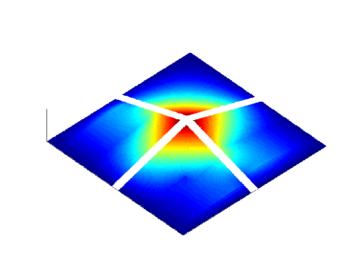
For each , we solve the spectral problem (9) and the first eigenfunctions are used to form the initial space. Each eigenfunction will be first multiplied by the partition of unity function , for each , and is then decoupled across coarse grid edges to form basis functions. In particular, the new basis functions have support in one of the coarse grid block forming and are zero in the other three coarse grid blocks forming . For example, if , the basis function is . We write as the space spanned by , for all . See Figure 2 for an illustration. The initial space is obtained by the linear span of all functions constructed in the above procedure.

3.2 Construction of online basis functions
In this section, we will discuss the construction of our local online basis functions. The purpose is to add basis functions locally in some coarse neighborhoods to obtain rapidly decaying errors. Assume that the space at the -th iteration and the corresponding solution are given. For each coarse neighborhood , we define the local residual by
| (11) |
where contains functions that are zero on . The residual can be seen as a linear functional defined on with norm defined by
and . We will then find the new online basis function by solving
| (12) |
The new online basis function is added to to form .
The motivation of finding a new basis function by solving (12) can be explained as follows. We define the A-norm by
We notice that the A-norm is equivalent to the DG-norm by Lemma 2.1. From (2) and (7), we have the following Galerkin orthogonality condition
| (13) |
Thus, we see that the following optimal error bound holds
| (14) |
We will enrich the space by adding a basis function in the space to form . First, (14) implies
| (15) |
Taking , for some scalar , in (15), we have
which implies
Taking , we obtain
| (16) |
By the definition of the residual in (11), we see that (16) becomes
| (17) |
From (17), we see that the quantity measures the amount of reduction in error when the basis function is added in to form . We will construct the function to obtain the most reduction in error. Thus, we find that maximizes . Equivalently, we find by solving
Notice that, we have used the fact that when .
3.3 Convergence of the adaptive procedure
In this section, we analyze the convergence of the above online enrichment procedure. We begin our analysis at the inequality (17). Notice that, this inequality can be written as
| (18) |
when the basis function is obtained as in (12).
On the other hand, we will show that the error can be controlled by the residual norm . To do so, we consider an arbitrary function . Let be the restriction of in , and let be the component of in the offline space . By the GMsDGM (2), the fine-grid problem (7) and the Galerkin orthogonality (13), we have
where we define and use the fact that for all . By (7), we have
Using the property for all ,
Writing the above sum over coarse neighborhoods , we have
For each coarse neighborhood , we define the following modified local residual by
| (19) |
The modified residual can be seen as a linear functional defined on with norm defined in the following way
In the above definitions, is considered to be defined only on , and has zero value outside .
Using the definition of the modified residual , we have
| (20) |
where we used the fact that is zero on . Using Lemma 2.1,
| (21) |
By the definition of the DG-norm,
| (22) |
For each , we have
| (23) |
For each , we have
| (24) |
Combining inequalities (23) and (24) in (22), we have
| (25) |
where . Using the spectral problem (9), we have
and
Hence, (20) becomes
We remark that the above inequality holds for any . Taking and using Lemma 2.1, we finally obtain
| (26) |
where and is the number of vertices of the coarse grid block .
We summarize the above results in the following theorem.
Theorem 3.1.
We remark that one can derive a priori error estimate for the error , for every . Since the purpose of this paper is an a posteriori error estimate (28) and the convergence of an adaptive enrichment algorithm (29), we will not derive a priori error estimate.
Finally, we remark that by using more basis functions in the initial space , the values of the eigenvalues are larger. Thus, the value of is further away from zero, and this fact enhances the convergence rate. In particular, the convergence rate is affected by the quantity . The convergence is slow when is small (cf. [8, 24]). We also remark that one can add online basis functions in multiple coarse neighborhoods to speed up the convergence. Let be the index set for which online basis functions are added in for . By using similar arguments as above, we obtain
where
4 Numerical Results
In this section, we will present some numerical examples to show the performance of the proposed method. The implementation procedure of online adaptive GMsDGM is described below. First, we choose a fixed number of functions for every coarse neighborhood by solving the local spectral problem. This fixed number for every coarse neighborhood is called the number of initial basis. After that, we split these functions into the basis functions of the offline space such that each basis function is supported in one coarse grid block. We denote this offline space as and set .
The coarse neighborhoods are denoted by , where and and and are the number of coarse nodes in the and directions respectively. We consider and as the set of odd and even indices from . Similarly, and are the set of odd and even indices from . In each iteration of our online adaptive GMsDGM, we will perform sub-iterations which add online basis functions in the non-overlapping coarse neighborhoods with , , and respectively.
We will take and . The domain is divided into uniform square coarse blocks. Each coarse block is then divided into fine blocks consisting of uniform squares. Namely, the whole domain is partitioned by fine grid blocks. The medium parameter is shown in Figure 3. The source function is taken as the constant 1.

To compare the accuracy, we will use the following error quantities
4.1 Comparison of using different number of initial basis
In Table 1, we present the convergence history of our algorithm for using one, two, three, four initial basis per coarse neighborhood. Notice that, in the presentation of our results, DOF means the total number of basis functions used in the whole domain. We use the continuous multiscale basis functions as the initial partition of unity. In the tables, we obtain a fast error decay which give us a numerical solution with error smaller than in two or three iterations. We can see the error decay of using one initial basis is slower than the error decay of using two or more initial basis since for using one initial basis is too small.
| DOF | ||
|---|---|---|
| 324 | 44.50% | 24.88% |
| 648 | 9.92% | 2.18% |
| 972 | 0.78% | 7.54e-2% |
| 1296 | 3.24e-2% | 2.13e-3% |
| 1620 | 2.42e-4% | 1.10e-5% |
| DOF | ||
|---|---|---|
| 648 | 17.73% | 3.58% |
| 972 | 0.31% | 1.80e-2% |
| 1296 | 3.52e-3% | 1.62e-4% |
| 1620 | 1.81e-5% | 8.58e-7% |
| 1948 | 1.04e-7% | 4.68e-9% |
| DOF | ||
|---|---|---|
| 972 | 11.30% | 1.72% |
| 1296 | 0.45% | 2.44e-2% |
| 1620 | 3.05e-3% | 1.37e-4% |
| 1944 | 1.06e-5% | 4.08e-7% |
| 2240 | 4.59e-8% | 2.14e-9% |
| DOF | ||
|---|---|---|
| 1296 | 8.38% | 1.00% |
| 1620 | 7.98e-2% | 3.13e-3% |
| 1944 | 9.93e-4% | 3.57e-5% |
| 2268 | 1.39e-5% | 5.15e-7% |
| 2540 | 4.23e-8% | 1.55e-9% |
Bottom-left: Three initial basis (). Bottom-right: Four initial basis ().
To further study the importance of the initial basis, we will present another example with a different medium parameter shown in Figure 4. The domain is divided into coarse blocks consisting of uniform squares. Each coarse block is then divided into fine blocks also consisting of uniform squares. The convergence history for the use of one, two, three, four initial basis and the corresponding total number of degrees of freedom (DOF) are shown in Table 2, Table 3, Table 4, Table 5 respectively. We consider two different contrasts. On the right table, we increase the contrast by 100 times. More precisely, the conductivity of inclusions and channels in Figure 2 (left figure) is multiplied by 100. In this case, the first 4 eigenvalue that are in the regions with channels become 100 times smaller. The decrease in the eigenvalues will slow down the error decay. In Table 2, we can observe that the error decay for the lower contrast case is much faster than the higher contrast case. In the higher contrast case, the error stop decreasing in some iterations. Similar observations are obtained when we use 2 or 3 initial basis. For using four initial basis, we observe a rapid convergence for both higher and lower contrast case.

| DOF | ||
|---|---|---|
| 64 | 25.44% | 6.67% |
| 128 | 1.20% | 0.23% |
| 192 | 0.47% | 0.10% |
| 256 | 0.26% | 5.79e-2% |
| 320 | 0.10% | 2.30e-2% |
| 384 | 6.22e-2% | 1.02e-2% |
| 448 | 3.70e-4% | 1.57e-5% |
| DOF | ||
|---|---|---|
| 64 | 25.45% | 6.67% |
| 128 | 1.45% | 0.27% |
| 192 | 1.39% | 0.27% |
| 256 | 0.84% | 0.15% |
| 320 | 0.34% | 7.98e-2% |
| 384 | 0.34% | 7.91e-2% |
| 448 | 0.15% | 3.71e-2% |
Right: Higher contrast(1e6)().
| DOF | ||
|---|---|---|
| 128 | 18.22% | 4.42% |
| 192 | 1.14% | 0.12% |
| 256 | 0.50% | 4.95e-2% |
| 320 | 4.17e-2% | 2.06e-3% |
| 384 | 5.73e-3% | 5.38e-4% |
| 448 | 7.12e-4% | 2.89e-5% |
| DOF | ||
|---|---|---|
| 128 | 18.56% | 4.62% |
| 192 | 1.37% | 0.16% |
| 256 | 1.25% | 0.14% |
| 320 | 1.23% | 0.13% |
| 384 | 0.41% | 3.22e-2% |
| 448 | 3.63e-2% | 3.56e-3% |
Right: Higher contrast(1e6)().
| DOF | ||
|---|---|---|
| 192 | 10.69% | 1.86% |
| 256 | 0.80% | 6.66e-2% |
| 320 | 0.34% | 2.24e-2% |
| 384 | 1.51e-2% | 6.24e-4% |
| 448 | 2.25e-4% | 1.61e-5% |
| 508 | 1.72e-6% | 6.70e-8% |
| DOF | ||
|---|---|---|
| 192 | 11.55% | 2.14% |
| 256 | 1.13% | 0.10% |
| 320 | 0.98% | 8.85e-2% |
| 384 | 0.96% | 8.95e-2% |
| 448 | 0.30% | 1.39e-2% |
| 508 | 2.00e-3% | 8.39e-5% |
Right: Higher contrast(1e6)().
| DOF | ||
|---|---|---|
| 248 | 7.92% | 1.14% |
| 312 | 0.25% | 2.42e-2% |
| 376 | 5.09e-3% | 2.72e-4% |
| 440 | 5.18e-5% | 2.62e-6% |
| 484 | 1.39e-6% | 6.40e-8% |
| DOF | ||
|---|---|---|
| 242 | 9.63% | 1.59% |
| 306 | 0.51% | 5.40e-2% |
| 370 | 1.38e-2% | 9.46e-4% |
| 434 | 2.10e-4% | 1.59e-5% |
| 494 | 1.74e-6% | 1.27e-7% |
Right: Higher contrast(1e6)().
4.2 Setting tolerance for the residual
In this section, we will show the performance for the online enrichment implementing it only for regions with a residual error bigger than a certain threshold. We consider the medium parameter shown in Figure 3. We show the results for using three different tolerances () , and . We will enrich for the coarse regions with residual larger than the tolerance. In Table 6, we show the errors when using initial basis function for tolerances , and . We can see that the convergence history in the first few iteration is similar to the result shown in previous section. Moreover, the energy error of the multiscale solution is in the same order of the tolerance and the error will stop decreasing even if we perform more iterations. Therefore, we can compute a multiscale solution with a prescribed error level by choosing a suitable tolerance in the adaptive algorithm. In Table 7 and Table 8, we show the errors for the last three iterations when using and initial basis functions respectively for tolerances , and . We have the same observation that the energy errors have the same magnitude as the tolerances.
| DOF | ||
|---|---|---|
| 324 | 44.50% | 24.88% |
| 648 | 9.92% | 2.18% |
| 924 | 0.81% | 7.72e-2% |
| 976 | 0.29% | 2.49e-2% |
| DOF | ||
|---|---|---|
| 324 | 44.50% | 24.88% |
| 648 | 9.92% | 2.18% |
| 972 | 0.78% | 7.54e-2% |
| 1176 | 4.12e-2% | 2.88e-3% |
| 1184 | 2.65e-2% | 1.57e-3% |
| DOF | ||
|---|---|---|
| 324 | 44.50% | 24.88% |
| 648 | 9.92% | 2.18% |
| 972 | 0.78% | 7.54e-2% |
| 1284 | 3.24e-2% | 2.13e-3% |
| 1364 | 2.56e-3% | 1.55e-4% |
| DOF | ||
|---|---|---|
| 648 | 17.73% | 3.58% |
| 964 | 0.33% | 1.85e-2% |
| 972 | 0.30% | 1.63e-2% |
| DOF | ||
|---|---|---|
| 648 | 17.73% | 3.58% |
| 972 | 0.31% | 1.80e-2% |
| 1136 | 2.53e-2% | 1.24e-3% |
| DOF | ||
|---|---|---|
| 972 | 0.31% | 1.80e-2% |
| 1248 | 3.99e-3% | 1.85e-4% |
| 1276 | 2.49e-3% | 1.19e-4% |
| DOF | ||
|---|---|---|
| 972 | 11.30% | 1.72% |
| 1248 | 0.50% | 2.57e-2% |
| 1276 | 0.24% | 9.98e-3% |
| DOF | ||
|---|---|---|
| 972 | 11.30% | 1.72% |
| 1296 | 0.45% | 2.44e-2% |
| 1436 | 2.60e-2% | 9.70e-4% |
| DOF | ||
|---|---|---|
| 1296 | 0.45% | 2.44e-2% |
| 1564 | 3.52e-3% | 1.56e-4% |
| 1576 | 2.49e-3% | 1.04e-4% |
4.3 Adaptive online enrichment
In this section, we will show the performance for the online enrichment implementing it only for regions that have a cumulative residual that is fraction of the total residual. We consider the medium parameter shown in Figure 4 (4 channels medium).
Assume that the local residuals are arranged such that
We only add the basis for the coarse neighborhoods such that is the smallest integer with
In Table 9, we present the error for the last iterations when using initial basis functions with the tolerance and . Comparing the result to the previous case, we can observe that this can use less number of basis functions to achieve a similar error. In Figure 5, we present the distribution of number of basis functions in coarse blocks, and see that the number of basis functions is larger near the channels (c.f. Figure 4). Thus, online basis functions can be adaptively added in some regions using an error indicator.
| DOF | ||
|---|---|---|
| 348 | 0.35% | 5.19e-2% |
| 368 | 0.27% | 4.03e-2% |
| 392 | 6.13e-2% | 9.34e-3% |
| 412 | 6.04e-3% | 6.60e-4% |
| 424 | 1.51e-3% | 1.25e-4% |

5 Conclusion
Though the use of offline basis functions is important for multiscale finite element methods, adding online basis functions in some regions can improve the convergence dramatically. The construction of online basis functions for various applications and discretizations require a careful analysis. In particular, as we have shown earlier [8] for GMsFEM within continuous Galerkin framework that one needs a certain number of offline basis functions in order to guarantee that the online basis functions can result to a convergence independent of physical parameters. In this paper, we develop an online basis procedure for GMsDGM that can provide a convergence independent of the contrast and small scales. Because multiscale basis functions are discontinuous across coarse-grid boundaries, we construct a special offline space as well as online basis functions. We show that our construction will guarantee a convergence independent of the contrast and small scales if we select a certain number of offline basis functions based on a local spectral problem. Furthermore, we apply an adaptive procedure to add online basis functions in only some selected regions. Numerical results are presented to back up our theoretical findings.
Appendix
In this section, we proof Lemma 2.1. Let be a coarse grid block and let be the unit outward normal vector on . We let be the space of continuous piecewise bi-quadratic polynomials defined in , and we denote by the restriction of the conforming space on . The normal flux is understood as an element in and is defined by
| (30) |
where is the harmonic extension of in . By the Cauchy-Schwarz inequality,
By an inverse inequality and the fact that is the harmonic extension of
| (31) |
where we recall that is the maximum of over and is the constant from inverse inequality. Thus,
This shows that
| (32) |
Next, by the definition of , we have
Notice that
For an interior coarse edge , we let be the two coarse grid blocks having the edge . By the Cauchy-Schwarz inequality, we have
| (33) |
Notice that
where , . So, summing the above over all , we have
Thus we have
| (34) |
Similarly, we have
Summing the above two inequalities, we have
| (35) |
This proves the continuity (5).
References
- [1] Assyr Abdulle and Yun Bai. Adaptive reduced basis finite element heterogeneous multiscale method. Comput. Methods Appl. Mech. Engrg., 257:203–220, 2013.
- [2] T. Arbogast. Analysis of a two-scale, locally conservative subgrid upscaling for elliptic problems. SIAM J. Numer. Anal., 42(2):576–598 (electronic), 2004.
- [3] S. Brenner and L. Scott. The Mathematical Theory of Finite Element Methods. Springer-Verlag, New York, 2007.
- [4] Scott Shaobing Chen, David L. Donoho, and Michael A. Saunders. Atomic decomposition by basis pursuit. SIAM Rev., 43(1):129–159, 2001. Reprinted from SIAM J. Sci. Comput. 20 (1998), no. 1, 33–61 (electronic) [ MR1639094 (99h:94013)].
- [5] C.-C. Chu, I. G. Graham, and T.-Y. Hou. A new multiscale finite element method for high-contrast elliptic interface problems. Math. Comp., 79(272):1915–1955, 2010.
- [6] E. Chung and Y. Efendiev. Reduced-contrast approximations for high-contrast multiscale flow problems. Multiscale Model. Simul., 8:1128–1153, 2010.
- [7] E. Chung, Y. Efendiev, and R. Gibson. An energy-conserving discontinuous multiscale finite element method for the wave equation in heterogeneous media. Advances in Adaptive Data Analysis, 3:251–268, 2011.
- [8] E. Chung, Y. Efendiev, and T. Leung. Residual-driven online generalized multiscale finite element methods. submitted, arXiv:1501.04565.
- [9] E. Chung, Y. Efendiev, and W. T. Leung. Generalized multiscale finite element method for wave propagation in heterogeneous media. arXiv:1307.0123.
- [10] E. Chung, Y. Efendiev, and G. Li. An adaptive GMsFEM for high contrast flow problems. J. Comput. Phys., 273:54–76, 2014.
- [11] E. Chung and W. T. Leung. A sub-grid structure enhanced discontinuous galerkin method for multiscale diffusion and convection-diffusion problems. Commun. Comput. Phys., 14:370–392, 2013.
- [12] W. Dorfler. A convergent adaptive algorithm for poisson’s equation. SIAM J.Numer. Anal., 33:1106 – 1124, 1996.
- [13] Martin Drohmann, Bernard Haasdonk, and Mario Ohlberger. Reduced basis approximation for nonlinear parametrized evolution equations based on empirical operator interpolation. SIAM J. Sci. Comput., 34(2):A937–A969, 2012.
- [14] L.J. Durlofsky. Numerical calculation of equivalent grid block permeability tensors for heterogeneous porous media. Water Resour. Res., 27:699–708, 1991.
- [15] W. E and B. Engquist. Heterogeneous multiscale methods. Comm. Math. Sci., 1(1):87–132, 2003.
- [16] Y. Efendiev and J. Galvis. A domain decomposition preconditioner for multiscale high-contrast problems. In Y. Huang, R. Kornhuber, O. Widlund, and J. Xu, editors, Domain Decomposition Methods in Science and Engineering XIX, volume 78 of Lect. Notes in Comput. Science and Eng., pages 189–196. Springer-Verlag, 2011.
- [17] Y. Efendiev, J. Galvis, and T. Hou. Generalized multiscale finite element methods. Journal of Computational Physics, 251:116–135, 2013.
- [18] Y. Efendiev, J. Galvis, R. Lazarov, M. Moon, and M. Sarkis. Generalized multiscale finite element method. Symmetric interior penalty coupling. J. Comput. Phys., 255:1–15, 2013.
- [19] Y. Efendiev, J. Galvis, R. Lazarov, and J. Willems. Robust domain decomposition preconditioners for abstract symmetric positive definite bilinear forms. ESAIM Math. Model. Numer. Anal., 46(5):1175–1199, 2012.
- [20] Y. Efendiev, J. Galvis, G. Li, and M. Presho. Generalized multiscale finite element methods. oversampling strategies. to appear in International Journal for Multiscale Computational Engineering.
- [21] Y. Efendiev, J. Galvis, and X.H. Wu. Multiscale finite element methods for high-contrast problems using local spectral basis functions. Journal of Computational Physics, 230:937–955, 2011.
- [22] Y. Efendiev and T. Hou. Multiscale Finite Element Methods: Theory and Applications, volume 4 of Surveys and Tutorials in the Applied Mathematical Sciences. Springer, New York, 2009.
- [23] Y. Efendiev, T. Hou, and V. Ginting. Multiscale finite element methods for nonlinear problems and their applications. Comm. Math. Sci., 2:553–589, 2004.
- [24] J. Galvis and Y. Efendiev. Domain decomposition preconditioners for multiscale flows in high contrast media. reduced dimension coarse spaces. SIAM J. Multiscale Modeling and Simulation, 8:1621–1644, 2010.
- [25] M. Ghommem, M. Presho, V. M. Calo, and Y. Efendiev. Mode decomposition methods for flows in high-contrast porous media. global-local approach. Journal of Computational Physics, Vol. 253., pages 226–238.
- [26] T. Hou and X.H. Wu. A multiscale finite element method for elliptic problems in composite materials and porous media. J. Comput. Phys., 134:169–189, 1997.
- [27] Dinh Bao Phuong Huynh, David J. Knezevic, and Anthony T. Patera. A static condensation reduced basis element method: approximation and a posteriori error estimation. ESAIM Math. Model. Numer. Anal., 47(1):213–251, 2013.
- [28] K. Mekchay and R. H. Nochetto. Convergence of adaptive finite element method for general second order elliptic PDEs. SIAM J. Numer. Anal., 43:1803–1827, 2005.
- [29] N. C. Nguyen, G. Rozza, D. B. P. Huynh, and A. T. Patera. Reduced basis approximation and a posteriori error estimation for parametrized parabolic PDEs: application to real-time Bayesian parameter estimation. In Large-scale inverse problems and quantification of uncertainty, Wiley Ser. Comput. Stat., pages 151–177. Wiley, Chichester, 2011.
- [30] Beatrice M. Riviere. Discontinuous Galerkin Methods For Solving Elliptic And parabolic Equations: Theory and Implementation. SIAM, 2008.
- [31] Timo Tonn, K. Urban, and S. Volkwein. Comparison of the reduced-basis and POD a posteriori error estimators for an elliptic linear-quadratic optimal control problem. Math. Comput. Model. Dyn. Syst., 17(4):355–369, 2011.
- [32] X.H. Wu, Y. Efendiev, and T.Y. Hou. Analysis of upscaling absolute permeability. Discrete and Continuous Dynamical Systems, Series B., 2:158–204, 2002.