The timing of life history events in presence of soft disturbances
Abstract
We study a model for the evolutionarily stable strategy (ESS) used by biological populations for choosing the time of life-history events, such as migration and breeding. In our model we accounted for both intra-species competition (early individuals have a competitive advantage) and a disturbance which strikes at a random time, killing a fraction of the population. Disturbances include spells of bad weather, such as freezing or heavily raining days. It has been shown in [24], that when , then the ESS is a mixed strategy, where individuals wait for a certain time and afterwards start arriving (or breeding) every day. We remove the constraint and show that if then the ESS still implies a mixed choice of times, but strong competition may lead to a massive arrival at the earliest time possible of a fraction of the population, while the rest will arrive throughout the whole period during which the disturbance may occur. More precisely, given , there is a threshold for the competition parameter , above which massive arrivals occur and below which there is a behaviour as in [24]. We study the behaviour of the ESS and of the average fitness of the population, depending on the parameters involved. We also discuss how the population may be affected by climate change, in two respects: first, how the ESS should change under the new climate and whether this change implies an increase of the average fitness; second, which is the impact of the new climate on a population that still follows the old strategy. We show that, at least under some conditions, extreme weather events imply a temporary decrease of the average fitness (thus an increasing mortality). If the population adapts to the new climate, the survivors may have a larger fitness.
Keywords: Evolutionarily stable strategy, fitness, climate change, extreme events, phenology
AMS subject classification: 28A25
1 Introduction
Proper timing of life-history events, like emergence, germination, migration or breeding, is crucial for survival and successful reproduction of almost all organisms. Timing may be set by endogenous rhythms or by extrinsic environmental clues (e.g. day length or temperature, [41]), but in almost all cases timing seems to have evolved according to two contrasting selective pressures. On the one hand, the first individuals that emerge or arrive at a given site often perform better, because they can profit from the better habitats and benefit from reduced competitions (at least for some time). On the other hand, however, early individuals may suffer from higher mortality, as they expose themselves to the risk of adverse environmental conditions, which usually are more likely early than late in the season. Autumn migration may seem an exception to this pattern, as the risk of mortality is probably larger for late than early departing individuals. However, in this case, migrants may benefit from a longer stay in their breeding grounds (allowing to rise a further brood or acquire larger fat reserves for migration). At the end, this pattern can be seen as the exact reverse of the process going on in spring, and can therefore be modelled in the same way.
In a seminal work Iwasa and Levin [24] have provided a first theoretical description of how the risk of incurring in adverse environmental conditions may shape the timing of life history events of a population, as a result of evolution over many generations. Under the assumption that adverse conditions (disturbance according to their definition, which we will follow hereafter) strike at a random time and are so strong that no individual incurring in the disturbance can survive, the authors show that (in many cases) the evolutionarily stable strategy (ESS from here on) is an asynchronous choice of times in the population. This asynchronicity has been observed in various settings and modelled by several authors (see [10], [12], [37], [38], [40] just to mention a few). In this paper we extend Iwasa and Levin’s model to the broader scenario where the disturbance is soft, meaning that it kills each individual with probability (in many cases some individuals in the population survive even to dramatic adverse conditions). The model of Iwasa and Levin can be seen as a particular case of ours when .
Before going into the details of our model, we have to mention that it focuses on the long time behaviour of a very large population. Indeed it is implicitly assumed that when the existence of mutants with better fitness is theoretically possible, then such mutants will appear and spread across the population. This does not take into account the disappearance (in finite populations) of certain alleles by mere random factors, a phenomenon which can be studied by means of mathematical population genetics (see for instance [19]). Long time behaviour of finite populations can also be studied through spatial models, namely interacting particles systems. Space not only adds complexity [18], but may also be interpreted as “type”, that is the location of one or more individuals can be seen as representing their genotype. For the simplest among this models, the branching random walk, much has been done: for instance in [5, 6, 8, 33, 46, 48] one finds characterization of the persistence/disappearance of genotypes (seen as locations for the model), on general space structures; the same can be found, for some random graphs, in [9, 36]. Stochastic modelling and interacting particle systems have been successfully applied to biology and ecology (see [2, 3, 4, 13, 14, 25, 26, 27, 29, 20, 49] just to mention a few). Although stochastic modelling is very interesting and complex, here we will assume that over many generations, our populations have been sufficiently large to justify the use of a model where stochasticity appears only in the random time at which the disturbance strikes.
As for terminology, in the present work the life-history events under study are arrival times, meaning that we focus on migratory birds and the time of arrival to their breeding grounds. This choice of words should not be considered a reduction in the scope of this paper, since our modelling approach is very broad, as it applies to the investigation of the timing of any life-history event when the benefits from being early and the risk of incurring in a soft disturbance are in conflict. Migratory birds are a well studied biological system where timing is crucial for the fitness of individuals, and where a long record of adverse conditions killing or impairing the reproduction of individuals exists (see e.g. [34]). Moreover the interest in the timing of these recurrent biological events is very strong among biologists after that several studies have consistently observed an advancement in arrival and reproduction of birds supposedly as a consequence of climate change (see [11], [16], [47]). Climate change not only implies warming temperatures, but also higher frequency and intensity of extreme meteorological events (see [22]). This increased weather unpredictability may severely affect migrant birds, because warmer springs prompt birds towards earlier arrivals, while more frequent unseasonable weather increases the risk of mass mortality events (see [43] for a stochastic model for random catastrophes striking a spatially structured population). It is widely accepted that climate change is endangering migrant populations (see [42]). Ornithologists therefore strongly need models investigating the contrasting forces affecting the timing of bird migration to improve their understating of the ongoing ecological processes and to plan better conservation strategies for declining migrant populations. We point out that even if our primary interest here are evolutionarily stable strategies which arise in large populations after many generations of stable climate (an equilibrium situation), our study also allows us to analyze some effects of a sudden climate change (an off-equilibrium dynamics). Indeed our results not only describe the ESS (Theorem 3.5) but also the effects of the climate change on the fitness of a population not yet adapted to the change (Propositions 3.7, 3.8 and 3.9).
Here is a short outline of the results of the paper. In Section 2 we introduce the model and the notation. We consider an intra-species competition regulated by a parameter and we define the fitness as a function of the arrival time conditioned on the disturbance time, the expected fitness depending only on the arrival time (averaged over all admissible disturbance times) and, later on, the average fitness (averaged over all disturbance and arrival times). We describe the meaning of an evolutionarily stable strategy (ESS) and we discuss the easiest cases where either there is no competition () or the probability of surviving the disturbance is 1, i.e. the disturbance has no effect whatsoever (Remark 2.1). Section 3 contains our main results. Theorem 3.5 extends [24, Appendix A] and shows that there is only one possible ESS for the population in response to a fixed disturbance distribution, which we imagine supported in . The behaviour of the ESS depends on the value of . Indeed there exists a function of , say , such that if then the population starts arriving after a date and there are arrivals every day until ; if then continuous arrivals starts at ; if then a fraction of the population arrives at time 0 and the rest arrives continuously starting from . The dependence on and of the fitness of individuals following the ESS is discussed; in particular we show (see Remark 3.6) that the theoretical maximum value of the average fitness is not attained by any ESS. This proves that, even though an ESS is a strategy that each member of the colony considers fair, it is not the best choice for the colony as a whole. The dependences of every relevant coefficient on , and the disturbance distribution are summarized in a table before the beginning of Section 3.1. As an example, we describe the case where the disturbance strikes according to a uniform distribution (see Section 3.1). The effects of climate changes are studied in Section 3.2. The main questions discussed here are the following. How does the ESS change after a climate modification? What happens if a population would keep the same strategy after a climate change? A worse climate, that is a smaller , may change the shape of the ESS delaying the first arrivals and increasing the fitness of each individual (provided that the population survives the transition). If the distribution of the disturbance is linearly rescaled, the same happens to the ESS. The behaviour of the fitness, before the strategy adapts, is studied in Propositions 3.7, 3.8 and 3.9. A consistent delay of the disturbance reduces the fitness of all individuals following the former ESS. If the disturbance arrives earlier than in the past, then the average fitness of the population increases. When the competition is weak then a decrease of implies a killing of a larger fraction of the population and hence a lower average fitness. In Section 4 we discuss and summarize the conclusion of the paper. Section 5 is devoted to the proofs of our results.
2 The model
Iwasa and Levine [24] studied different ways to model the fact that individuals choosing an early date of arrival, if no disturbance were present, would obtain a larger fitness than those arriving later. This may be due to the fact that a decrease of reproductive success (better resources at earlier times, [24, Case 1]) or to competition between individuals, for instance those who arrive earlier may feast on food, while those arriving later will not ([24, Case 2]). We focus on the second case, where Iwasa and Levin proved the emergence of a mixed strategy for the arrival dates (which is more interesting and realistic than Case 1, where all individuals choose the same date).
Suppose that is the probability measure, supported on , according to which individuals choose the date of arrival to the breeding sites. Its cumulative distribution function is defined, as usual, by for all . The population is struck by a single disturbance (e.g. storm, frost) whose date is randomly distributed on with density . It may be that ( is the first possible date of disturbance while is the last). Individuals already present when the disturbance occurs, survive with probability . The fitness of an individual is a decreasing function of the fraction of individuals (in the whole population) who are already present when it arrives, and of the parameter which represents the strength of intra-species competition. Inspired by [24] we choose the following expression for the fitness of an individual arriving at date , given that the disturbance strikes at time :
Thus is the fitness (under the strategy ) of an individual arrived at time when the disturbance strikes at time . It is worth noting that we are implicitly exploiting the Law of Large Numbers (LLN), since the exact value of , for instance if , is
where is the random number of individuals arrived before and is the population size. If is large, the LLN implies that can be approximated by . Similarly one proceeds with the case .
We consider the expectation of the fitness, with respect to the disturbance date: the expected fitness of an individual arrived at is
More explicitly, for ,
| (2.1) |
We note that, in the last integral of equation (2.1) (as well in every integral of a function of type in the sequel), one could use instead of and the value of the integral would be the same (as the definition of ); moreover if , by we mean .
We assume that, the population follows evolutionarily stable strategies, that is, distributions of arrival times which grant no advantage to any particular choice of arrival date. More precisely, an evolutionarily stable strategy (ESS) , is such that no mutant can have an advantage, namely for all and for all , . This implies that for all , where . We recall that is the (closed) set of such that for all . We will also need to define the essential support of a real function , which is the support of the associated measure (for instance, if is continuous then ). We recall that in [24] the probability distribution of the disturbance was considered as absolutely continuous with a single peak density which was taken, on as a polynomial vanishing at the extrema of the interval. We only assume that is a probability density, supported in . From now on, without loss of generality, we assume and .
We are interested in studying as a function of and (and of , but here is thought as fixed). The extremal cases where either or are easy to describe.
Remark 2.1.
- 1.
If and , there is no competition and the disturbance has no effect. Then for all ; moreover, every is an ESS (indeed the disturbance has no chance to shape an evolutionary response of the species).
- 2.
If and , there is no competition. From equation (2.1) we have, which is non decreasing and continuous and for all . We see here that there is no dependence on . A probability measure is thus an ESS if and only if . This means that all idividuals will arrive after the last possible date of disturbance.
- 3.
If and , there is competition and the disturbance has no effect. From equation (2.1) we have which is right-continuous and nonincreasing. Using the same arguments as in the proof of Theorem 3.5 it is straightforward to prove that there is a unique ESS, namely . Everybody arrives at the first possible arrival date (indeed there is no risk in doing so).
- 4.
The interesting case is when and , that is, competition in the population and effective disturbance. These are the constraints which we assume thereafter.
3 Main result
We are able to prove (Theorem 3.5) that given , there exists a critical , depending only on (not on ) such that:
- 1.
- 2.
if then the ESS is as before, with (individuals arrive throughout the whole period of possible disturbance, see for instance Figure 10);
- 3.
if then the ESS is such that a fraction of individuals arrive at 0, and the remaining arrive continuously during the whole period of possible disturbance (see for instance Figure 10).
Before stating our main result, we define the quantities , and .
Definition 3.1.
If , then ; if , then is the solution to the equation
| (3.2) |
Note that the solution to equation (3.2) exists and is unique since the l.h.s. is a continuous, strictly increasing function of which vanishes at and goes to infinity as . The inverse function of will be denoted by (by definition ). Clearly (resp. ) if and only if (resp. ).
Definition 3.2.
If let . If define as the maximal solution to the equation
| (3.3) |
Note that the solution to equation (3.3) exists and is unique, since the r.h.s. is positive and strictly smaller than 1, while the l.h.s. is a continuous, nonincreasing function of which takes values and at and respectively. By definition if , .
Definition 3.3.
If let . If let be the unique solution to the equation
| (3.4) |
The solution exists and is unique since the l.h.s. is a continuous, strictly decreasing function of which takes values in when and is equal to when . Observe that for all .
Note that, in accordance with [24], if then , , and . Let us discuss some general properties of , and . For details on the proofs, see Section 5.
Remark 3.4.
- 1.
The map is continuous and strictly decreasing; see Figure 1. By using elementary techniques of implicitly defined functions it is not difficult to prove that , .
- 2.
Given a fixed , we have that and are strictly decreasing and left continuous everywhere. The map is right continuous at only in the following cases: (a) ; (b) and for some ; (c) and . Similarly is right continuous at only in the cases: (a) ; (b) and for some ; (c) and . Again using standard techniques of implicitly defined functions we have
(3.5) - 3.
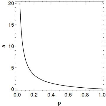


Theorem 3.5.
Let , and be as previously defined. Given , and a probability density supported in (where by definition ), there exists a unique ESS . In particular, , where is an absolutely continuous probability measure with . The cumulative distribution function is implicitly defined, on , by
| (3.6) |
The value of (the supremum of ) is
| (3.7) |
Finally, is a phase transition value for the competition in the sense that
It is worth noting that, in equation (3.6), we can write instead of .
Several features of the ESS can be read from Theorem 3.5. Beside arrivals at 0 (possible only when competition is sufficiently strong), individuals arrive only at possible disturbance dates. This means that if it is certain that during , no disturbance is possible (i.e. for all ), then the probability of arrivals in such interval is zero. This is due to competition, which advantages early birds: there is no point in choosing to arrive in between and , since there is no risk in choosing instead.
In most real cases, one may assume that on . In that case individuals will arrive either (1) avoiding the first part of the possible time period (weak competition, see Figure 19) or (2) during the whole interval without massive arrivals at 0 (critical competition, Figure 19) or (3) during the whole interval with massive arrivals at 0 (supercritical competition, Figure 19).
The first arrival time is strictly decreasing with respect to and to (Remark 3.4); this means that strong competition and/or high probability of surviving the disturbance, push arrivals to 0. If is fixed, competition needs to be above the threshold , in order to have arrivals at 0. On the other hand, if competition is fixed, only weak disturbances lead to early arrivals.
As for , the fraction of arrivals at 0, we know that it increases with . If , from equation (3.6), using as , it follows that for all as . This means that, as the competition increases, given that an individual does not arrive at time (this probability converges monotonically to from above) then the probability of arriving after goes to , that is, in the limit as the arrival distribution converges to (that is, if ). Note that this does not happen when : in that case which implies that converges to the cumulative distribution of the disturbance arrival time.
Associated to a given strategy , there is the average fitness . In particular when is an ESS, then for all (where , see (3.7)), hence . If we can relate to : by equations (3.3) and (3.7) we have
| (3.8) |
It is not difficult to prove that is continuous in ; moreover and are strictly decreasing functions (see Remark 5.3) such that
hence for all ; moreover .
Thus, when is an ESS the average fitness is decreasing with respect to (when ), hence, if we think of the fitness as a probability of survival, the average rate of survivors is decreasing if the chance of surviving the catastrophe is increasing. From a biological point of view, this model suggests that, in the presence of competition, if the disturbance is weaker (that is, increases) then the ESS pushes the colony towards an early arrival on the site, increasing the negative effects of the competition on the fitness (which overcome the positive effects of the weaker disturbance). Hence the stronger the disturbance the higher the average fitness corresponding to the ESS (in some sense, if we think of the average fitness of the population as its “strength”, a strong disturbance will select a stronger population).
![[Uncaptioned image]](1504.04272v2/lambda-a-01.jpeg)
![[Uncaptioned image]](1504.04272v2/lambda-a-03.jpeg)
![[Uncaptioned image]](1504.04272v2/lambda-a-08.jpeg)
![[Uncaptioned image]](1504.04272v2/lambda-05-p.jpeg)
![[Uncaptioned image]](1504.04272v2/lambda-2-p.jpeg)
![[Uncaptioned image]](1504.04272v2/lambda-3-p.jpeg)
One may wonder if there are strategies which (given the environment ) lead to a larger , and whether these strategies are Evolutionary Stable Strategies.
Remark 3.6.
The supremum of the map is and is attained by if and only if and is continuous (and this supremum holds for any fixed , see details in Section 5). This means that the best choice for the population as a whole, is to start arriving after the last possible date of disturbance. In particular no ESS can attain this maximum value (an ESS is supported in ). An ESS is a strategy which is well accepted by every individual (since the fitness is constant and maximal), while the maximizing strategies imply that some individuals“accept” a lower fitness for the benefit of the whole colony (note that the continuity of implies that the population cannot choose to arrive simultaneously at , which would guarantee the same fitness for everyone). Moreover, even if the maximal fitness is attained only arriving after , it is possible to prove that we can find a sequence of strategies (not ESSs) , supported in such that . In Figure 4 the dashed line represents , whereas the dotted and the solid ones are the average fitness when the population follows the ESS, and , respectively. The filled region represents all possible values for with . Note that following the ESS a population cannot achieve the maximal average fitness, nevertheless if is either small or large, then the dashed and the solid line are close, hence, if or at least is small, then the average fitness is not so far from its theoretical supremum.

In the following table, we summarize the main properties of the coefficients , , and ; by and we mean that a particular coefficient is increasing or decreasing with respect to the parameter .
| Coefficients | Dependence | Properties |
|---|---|---|
| Phase transition competition | ||
| Probability of emigration at time , | , | |
| if | ||
| if | ||
| Fitness of individuals for the ESS, | , | |
| Maximum average fitness for a generic strategy | ||
| Earliest arrival time for an ESS | , , | |
| if | ||
| if |
Given , Theorem 3.5 gives the unique ESS and its average fitness . We note that the map is not injective. Indeed, at least when , it might be that for some and . Even if we fix , at least in the subcritical case, different disturbance distributions may lead to the same ESS. Indeed, suppose that then and . Given is fixed, from equation (3.6), is uniquely determined on . Nevertheless, on the only constraint is , which can be satisfied by infinitely many distributions. This means that different levels of competition, and/or of climate, can lead to the same response and same fitness .
3.1 Uniformly distributed disturbances
In this example we suppose that , that is, the law of the disturbance is uniformly distributed in the interval (we also write ). In this case some explicit computations are possible.
The coefficients , , do not depend of ; the only coefficient depending on is the first time of arrival (which is nonzero only if ). If , then
where , with . This means that, in the subcritical case, the ratio between the length of the arrival times interval and that of the disturbance times interval, depends only on and (not on ); indeed .
The cumulative distribution function can be computed using equation (3.6). Although when no explicit evaluations are possible, one can see that is a rescaling of the cumulative distribution function of the ESS obtained when the disturbance is uniformly distributed on the interval [0,1] (with the same parameters and ), which we denote by . More precisely, if is the cumulative distribution function of the ESS when , then
| (3.9) |
(recall that if while if ). Using computer-aided numerical solutions, in Figures 10–10 we plot the cumulative distribution functions of the ESS (solid line) and of the disturbance (dashed), with different parameters and disturbance intervals. In the first row, Figures 10–10, we take while in the second row, Figures 10–10, we have .
In the three figures in each row, the parameters are, respectively, , and . This implies that the first figure represents a subcritical case (). Note that in both rows in this case the arrivals start towards the end of the disturbance intervals and the ratio between the length of the two intervals representing the arrival times and the disturbance time is the same, .
The second figure of the row is a supercritical case (), where a fraction of the population arrives at time 0. In both rows the fraction is the same ( depends only on and ).
The third figure is again a supercritical case (), where strong competition forces a larger fraction of the population () to arrive early. Along with the values of and , in Figures 10–10 we write the explicit value of the maximum average fitness . Note that increases when either decreases or increases, the maximum competition .


As we have seen in Figures 10–10, by (3.9), it is enough to study the case . In Figures 19-19 we plot the cumulative distribution function (solid line) corresponding to nine couples , together with the cumulative distribution function of the disturbance (dashed line). In each row takes the same value ( and in the first, second and third row respectively), while is constant along each column ( and in the first, second and third column respectively). In this way, figures on the diagonal represent critical cases, figures on the upper triangle are subcritical cases and figures on the lower triangle are supercritical cases.


3.2 Climate changes
In our model the climate can be represented by the couple , that is, the distribution and the strength of the disturbance; more precisely the lower the stronger the disturbance. One can argue that also the competition parameter could be affected by the climate, nevertheless, in this paper, we prefer to think of it as a characteristic of the population.
When climate changes (i.e. the couple changes), there are two interesting questions.
- 1.
How does the ESS change reflects a climate change? In other words, can we predict in which respect the new ESS will differ from the previous one?
- 2.
What happens if a colony keeps the same strategy of arrivals after a climate change? Does the average fitness of the population decrease or increase?
Some answers can be obtained if we imagine that the climate change affects just one of the parameters and .
The answer to question 1, is given by Theorem 3.5. If decreases, then increases: after the population has adapted to the new climate the common fitness will have increased (of course supposing that the population is sufficiently large to survive the transition period). Moreover, a decrease of may lead from an ESS with massive arrival at 0, to an ESS with arrivals after a date . Let us discuss now what happens if changes, that is if it moves from to . The fitness of every individual, according to an ESS adapted to , is which does not depend on , thus that will not change in case of rapid adaptation (question 1). What will change is the distribution of the arrival times and possibly its support. In the case of uniformly distributed disturbances, the answer to question 1 is given by equation (3.9): a change of the interval during which disturbances occur is simply reflected by a rescaling of the ESS. It is worth noting that an analogous result holds if we take a generic density defined on and we rescale it as follows
| (3.10) |
the effect on the ESS in this general case is still the rescaling given by equation (3.9).
The second question is particularly interesting in the case of rapid climate changes, since the adaptation of the population (moving from the old ESS to the new one) could require several generations; thus the changes may endanger the survival of the population. A sudden change of climate may be an advantage for some individuals (i.e. some arrival dates) and a disadvantage for other individuals. Even in the case of a simple anticipation of the disturbance the situation is not trivial. Suppose that is supported in and is supported in , with . Individuals arriving at are sure that the disturbance is over but they might have more competitors still alive (for instance those arriving at ), thus it is not clear whether the climate change implies a larger or smaller fitness. The following proposition gives a partial answer: let us denote by the fitness of an individual, in a population following the strategy (not necessarily an ESS), which chooses the arrival date and has to face the disturbance which is regulated by . If is a delay of the disturbance, that is, in the second scenario disturbances strike later in the season, early birds suffer a decrease of their fitness. The second part of the proposition tells us that, at least for uniform disturbances, if delays the beginning of the disturbance but also anticipates the end of the disturbance season, then later birds have an advantage.
Proposition 3.7.
Consider a distribution and two densities and on the intervals , .
- 1.
If then for all .
- 2.
If is the ESS associated to , is a random variable with density and is sufficiently small then for all .
- 3.
If and are uniform densities and and then for all (where ).
Proposition 3.7(1) and (3) follow from a more general result (Proposition 5.8) which allows to compare and in more general settings. Proposition 5.8 is fairly technical and can be found in Section 5. Proposition 3.7(2) implies for instance that a consistent delay of the disturbance (think of ) reduces the fitness of all individuals following the former ESS. Even if it is not necessary that , the requirement that is sufficiently small, implies that .
It is not trivial to assess whether individuals that profit from the climate change represent a small or large fraction of the population following what was a former ESS. More precisely, it is not always clear whether the average fitness increases or not. Nevertheless it is not difficult to provide some partial answers in the case of delay or anticipation of the disturbance.
Proposition 3.8.
Consider two densities and on the intervals , and let be the ESS associated to . Denote by a random variable with density .
- 1.
provided that is sufficiently small.
- 2.
provided that is sufficiently small.
Proposition 3.8(1) implies that a consistent delay of the disturbance reduces the average fitness of the population; on the other hand, Proposition 3.8(2) implies that the average fitness of the population increases if the disturbance arrives so early that most of the population has not yet arrived when the danger is over.
Let us discuss now the consequences of a change of . In the previous sections we showed that is decreasing. This means that if decreases and there is an instantaneous adaptation of the population to the new conditions (i.e. the arrival distribution changes accordingly) then the fitness of each individual (hence the average fitness) increases, because more individuals will choose to arrive later in the season. Intuitively, if the population does not adapt to the climate change, a decrease of should imply a killing of a larger fraction of the population and hence a lower average fitness. The following result tells us that this intuition is correct, at least for weak competition.
Proposition 3.9.
Given a generic arrival strategy , recall the definition of the average fitness as . The function is continuous in . Moreover for all we have for all and the inequality is strict if and only if for some .
This means that, if the competition is low, then when the probability of surviving the disturbance decreases then the fitness decreases as well. Roughly speaking, in case of low competition it is better to arrive later (and to have more competitors) than to take a chance against the disturbance.
4 Discussion
In this paper we developed a model for the timing of life history events when a disturbance can strike a population of migrators and may kill some of the individuals that incur in it. Our model therefore considered the biologically realistic scenario of a “soft” disturbance, i.e. an event, like extreme unseasonable weather, that can kill a fraction of the population, but to which some individuals survive. We developed our study by considering migratory birds as a model, because they are biological system where the timing of life history events has been intensively studied. In particular, we looked for the ESS for individuals that have to choose arrival time to their breeding grounds, and benefit from early arrival, as is often the case for migratory birds ([17]). On the other hand, they may incur in a catastrophe, for instance a spell of cold weather, that will kill a fraction of individuals that have arrived to their breeding grounds before the catastrophe. Clearly, the choice of focusing on arrival to the breeding grounds is purely exemplificative, and our model applies more generally to the timing of almost any life-history event. For example, it applies to timing of arrival to the wintering grounds, crossing of a geographical barrier like a mountain range, or to timing of reproduction, rather than arrival. From a biological point of view, the most interesting results we obtained can be summarized as follows. First, in presence of competition, a fraction of individuals arrive early during the season, in a period when they can incur in a catastrophe and therefore be killed. Interestingly, the stronger the competition, the earlier birds start arriving and may even arrive at the earliest time possible. Remarkably, there is a threshold value for the intensity of the competition above which a fraction of individuals arrive extremely early, i.e. at a time when they will certainly incur in the catastrophe. Hence, competition is able to force individuals to risk death if the payoff for an early arrival is sufficiently high. Second, a strong disturbance increases the fitness of individuals (fitness is equal for all individuals that follow the ESS) because, under a strong disturbance, the fraction of individuals arriving at a time when they can incur in the catastrophe decreases. Hence, a strong disturbance determines a later average arrival of the population. Actual distribution of arrival dates is therefore the balance between the contrasting pressures of competition and risk of death due to the catastrophe. Third, the ESS is not the strategy that determines the maximum average fitness of individuals in the population. Indeed, a larger average fitness could be obtained if some individuals would accept a reduction in their own fitness for favouring other individuals. This result is not surprising since individuals are predicted to behave selfishly and adopt the strategy that maximizes their own fitness. We also tested our model under a climate change scenario, which is predicted to increase the frequency and strength of extreme meteorological events ([23]), like spells of unseasonal weather that can kill migratory birds. We obtained two further interesting results. Fourth, climate change, which is predicted to increase the strength of the disturbance, should determine an increase in the fitness when individuals are able to adapt their arrival times to the new ESS (second result above). However, the ESS implies a later average arrival of individuals (third result above). Differences among species or populations in the observed shifts in the timing of migration according to climate change may therefore be due to differences in the susceptibility of species or populations to extreme weather conditions, which in our model is accounted for by the strength of the disturbance. Since climate change is determining on the one side a general advancement of the timing of spring events ([30, 45]), but on the other side it also increases the frequency of cold spells in spring ([21]), differences in the response of bird species or populations to climate change should be investigated also in respect to their susceptibility to unseasonable weather. Fifth, if the population is unable to adjust arrival times and continues following the previous timing, which is no more an ESS, the fitness of individuals declines (in many scenarios). It has been hypothesized that many migratory bird species, particularly long distance migrants, may be less able than short distance ones to advance their arrival to the breeding grounds because they are constrained by the timing of other life-history events ([32]). Consequently, they are forced to follow an arrival strategy that differs from the current ESS, and should suffer a reduction in fitness. Our model therefore gives an explanation of the possible mechanisms linking response to climate change and population trends and explaining why bird populations that did not show a response to climate change are declining ([31]). There is currently debate among biologists on whether the observed changes in arrival dates of migratory birds can be attributed more to micro-evolutionary processes or to phenotypic plasticity ([15]). If the response to climate change is due to phenotypic plastic response of individuals, then probably adaptation will be fast enough to keep the pace of climate change. In contrast, if timing of life history events is genetically controlled, a longer time may be needed for the new ESS to fix in the population, and in the meanwhile individual fitness will be reduced. In summary, the model we developed may contribute to our understanding of the processes determining the timing of life history events under the biologically realistic scenario of a catastrophe killing only a fraction of the individuals that incur in it. Our model explains how competition can induce a fraction of the population to arrive very early, despite facing a higher risk of death, as it is documented in several species ([35]). Moreover, our model also investigated the effect of climate change on the timing of life history events, and demonstrated that fitness should decline in a scenario of increased probability of catastrophe if the population is not able to adapt to the new climatic conditions.
5 Proofs
In this section one can find all the proofs of our results and some details about the remarks of the previous sections. We start with a lemma and its corollary.
Lemma 5.1.
Let , and be such that for all , for some , for all and for all . Define and
Then is a nondecreasing function on . Moreover is strictly increasing on if and only if there exists such that and .
Proof.
Note that is continuous on and differentiable on . We compute the derivative on as
Now and, by using ,
Since for all such that we have that for all , hence is non-decreasing.
Moreover, if and then and (just take ). This implies for all , whence is strictly increasing on . On the other hand if for all such that , clearly for all . ∎
Corollary 5.2.
Suppose that and . The the function is strictly increasing in .
Proof.
Apply Lemma 5.1 using , for all , for all and . ∎
The following is a brief remark which proves some of the properties of the functions and (the others are straightforward).
Details on Remark 3.4.
Most of the results about the functions , , and follow easily by checking the monotonicity and the the continuity (in each variable separately) of the l.h.s. and r.h.s. of the defining equations. We highlight just the main details.
- 1.
Since the l.h.s. of equation (3.2) is strictly decreasing, continuous with respect to and strictly increasing, continuous with respect to and since the r.h.s. is strictly decreasing, continuous with respect to we have that is strictly decreasing and continuous. As for the limit we note that, for every fixed ,
since pointwise in the first case and the Bounded Convergence Theorem applies, while pointwise in the second case and the Monotone Convergence Theorem applies. The limits follow easily by standard arguments.
- 2.
Since the r.h.s. of equation (3.3) is strictly increasing and continuous with respect to and with respect to and since the l.h.s. is continuous and nonincreasing with respect to we have that the maps and are strictly increasing. As for the continuity, note that, by definition, for every we have hence
These inequalities imply that, eventually, the maximal solution (resp. ). The limits from the right can be treated analogously by carefully dealing with the intervals where is constant.
Let us prove the limits in equation (3.5). By using the monotonicity of , we have that . Since the r.h.s. of equation (3.3) equals when we get that . In order to compute the second limit we observe that the r.h.s. of equation (3.3) tends to as . As for the second line in equation (3.5), note that for every we have that hence eventually as .
- 3.
The continuity follows from the continuity of the r.h.s. of equation (3.4) with respect to , from the continuity of the l.h.s. with respect to , and and from the monotonicity with respect to .
Let us prove that . We define and we can assume . Clearly, as . Hence for every fixed and and for every we have
eventually as . Hence
thus for every , satisfying , eventually as , the solution to equation (3.4), that is , satisfies . This implies .
In order to prove that for all , , it is enough to show that for all , . Indeed, in that case, the solution of satisfies (note that is strictly decreasing for all ). Observe that
where
When we have , hence it is enough to prove that , that is, . The first case is ; thus, which attains its maximum value (in ) at and . The second case is where . Note that , for all and as . Hence admits a global maximum in , which must be a stationary point since is differentiable. By taking the derivative we have that a stationary point must satisfy . Hence . This proves that for all and .
Now we prove that is strictly increasing in for all . Since is strictly decreasing for every fixed , it is enough to prove that is strictly increasing (for fixed ) to obtain that is strictly increasing where it is defined by equation (3.4) (by standard arguments for implicitly defined functions). By continuity it is enough to prove that where (the case would follow easily).
To this aim, let us replace the variable in the integral defining in the following way: where and (note that since ). This implies that when then and when then . Whence
Observe that . Moreover
which is strictly increasing with respect to since . Hence is nonincreasing (since ) and is strictly increasing. This implies that, for all ,
where in the second inequality we used for all , while in the last inequality we applied Corollary 5.2 (since ). Finally, this yields
∎
Remark 5.3.
The continuity of the function is easy. In the interval the function is strictly decreasing since the integral in the r.h.s. of equation (3.7) is strictly increasing for all . If then, using equation (3.4), we have that is a solution to
and, since the l.h.s. of this equation is strictly increasing with respect to and , standard arguments imply that is strictly decreasing.
We show now that is strictly decreasing. Let us start with the first expression in equation (3.7). In the following equation it is easy to show that the derivative with respect to and the integral with respect to commute and
for every since the integrand is strictly positive for every ; indeed the function is differentiable in and continuous in and the derivative is for all . This implies that is strictly decreasing for every fixed .
Let us consider now the second expression for , namely , which holds for where we recall that is the unique solution for with respect to . From equation (3.4) we have that, for every fixed , the function is implicitly defined by the equation where
The solution to the previous equation is uniquely defined in since is strictly increasing for every fixed and , . We can compute, using similar arguments as before,
where in the last equality we used the fact that, since , then . The last inequality holds since . By standard arguments, implies that is strictly decreasing for every .
Before proving Theorem 3.5, we prove that an ESS is of the form , where is an absolutely continuous probability measure.
Lemma 5.4.
Let be an ESS and fix . Then for some , , where is an absolutely continuous probability measure. Moreover and if then . Finally, is constant on and equals .
Proof.
We already noted that we can write equivalently
since . From this equation we can see easily that is right-continuous on ; moreover it is left-continuous at if and only if . If is such that then , if and only if . Indeed,
| (5.11) |
As a consequence, if then if and only if . Moreover if is such that , for all and then and . The first assertion, namely , comes from the fact that the support of a measure is a closed set. Suppose, by contradiction, that is an atom; clearly for all , since is an ESS, and hence which is a contradiction. This proves that the only atom, if any, of must be . Thus , where and is nonatomic.
We prove now that if , and , then ; this implies . By contradiction if there exists such that . Let then . Since , . Clearly , as a consequence of equation (5.11), . Hence there exists such that but this contradicts the definition of ESS.
Let us prove that . Observe that, for every we have
On the other hand, if , there exists such that and . This implies which contradicts the definition of an ESS. Thus .
If then and . On the other hand, , that is, . Since when we have , then which implies .
We are left to prove that is absolutely continuous. First of all we note that, from equation (2.1), where
is absolutely continuous and nondecreasing on . Since the only atom of , if any, is and is right-continuous, clearly is continuous on . It is well-known that any open set in can be decomposed into a disjoint, at most countable union of open intervals, hence where is an at most countable disjoint union of open intervals in . By definition, for all . Since then for all . As a consequence of equation (5.11), is constant on such intervals , but, since the value of at the extremal points of is , then for all . This proves that for all . Hence for all which implies
| (5.12) |
By composition, is clearly absolutely continuous on . Hence is absolutely continuous on (since for all ) and this implies that is an absolutely continuous measure (since ). ∎
Given a measurable subset , we denote by the set of real, measurable functions on which are integrable with respect to the Lebesgue measure. When a different measure needs to be specified, we write instead.
Remark 5.5.
A well-known characterization which will be used in the sequel is the following Lebesgue’s fundamental theorem of calculus (see for instance [39, Theorem 7.18]). A function is absolutely continuous on a compact interval if and only if there exists a function such that for some ( for all) and for all , ; in that case, for almost every , is differentiable at and .
This implies that an absolutely continuous function on is constant if and only if for almost every .
Moreover consider two functions , ; if is absolutely continuous and is monotone and absolutely continuous then is absolutely continuous. Similarly, if is a Lipschitz function and is absolutely continuous then is absolutely continuous. If is absolutely continuous then is absolutely continuous and the same holds for if is compact.
Finally if is differentiable everywhere and is differentiable almost everywhere clearly we have almost everywhere and, if in addition is absolutely continuous,
| (5.13) |
for all . If, in addition, is absolutely continuous then
| (5.14) |
A function is locally Lipschitz on if and only if for every there exists and such that , implies . By elementary analysis, if is a locally Lipschitz function on and is compact then there exists such that for all we have (that is, is globally Lipschitz on every compact subset of ). It is easy to show that a locally Lipschit function on is absolutely continuous on (one can prove it on every compact subset and then use the fact that is the union of an increasing family of compact subintervals). Hence the following result holds.
Proof of Theorem 3.5.
By Lemma 5.4, we know that an ESS can be written as , where is an absolutely continuous measure and , where (we will show later that ). Since for all , we have that is absolutely continuous on .
Since is absolutely continuous, we can take the derivative of in (2.1), for almost every ,
| (5.15) |
where is the derivative of . From now on it will be tacitly understood that the derivatives and equalities involving them, are defined and hold almost everywhere. From Lemma 5.4 we know that for all we have hence . Thus
Let . Using the last result of Remark 5.5 (by taking , and ), the previous equation is equivalent to
which, since for all , is in turn equivalent to
with the condition . By Remark 5.5, this is equivalent to
| (5.16) |
which, once we prove that , is equivalent to equation (3.6). This proves that given , is uniquely defined by the previous equation. From the previous equation, for all ,
which implies that . Now, since , from Lemma 5.4 we have that either (hence and ) or and . In this case and .
In particular, since , when (that is, ) we have that . Clearly the measure is supported in , but it is a probability measure if and only if , therefore, by using equation (5.16), and must satisfy
| (5.17) |
We note that . If then hence, from equation (5.12), by continuity of at we have , that is
| (5.18) |
since for all .
Let . If then by equation (5.17) and the discussion thereafter,
which is a contradiction. If then by plugging the explicit value of into (5.17), we get (3.3) (with instead of ) and since we showed that , thus it must be the (unique) maximal solution to equation (3.3), that is . This proves that implies and . Since the r.h.s. of equation (3.3) is strictly less than 1 (resp. equal to 1) when (resp. ) then equation (3.3) yields (resp. ). In order to obtain the first line of equation (3.7) just consider the expression of given by the r.h.s. of equation (3.3) and plug it in equation (5.18) (recalling that ).
Let . If then, by the definition of , equation (5.17) and the discussion thereafter,
which is a contradiction. If then (which coincides with the definition of given before equation (3.3)) and by plugging the explicit value of in equation (5.17) we have
which has a unique solution . Note that the r.h.s. of the equation is a decreasing continuous function of , say ; moreover by (3.2) and
This implies that the unique solution ; was proved in Remark 5.3. ∎
Before giving the details on Remark 3.6 we need a Lemma and another remark.
Lemma 5.6.
Let and be two finite measures on . Then the following conditions are equivalent:
- (1)
for every nondecreasing, measurable ;
- (2)
for every and ;
- (3)
for every nonincreasing, measurable ;
- (4)
for every and .
If one of these conditions holds we write .
Moreover the inequality in (1) is strict if and only if there exists such that (that is, if and only if there exists such that ).
Finally the inequality in (3) is strict if and only if there exists such that (that is, if and only if there exists such that ).
Proof.
The equivalence between (1) and (2) (or between (3) and (4)) is a classical result of measure theory: it is a slight modification of the arguments in [44, Section 1.A.1]. Moreover, to prove that just take condition (1) (or condition (3)) and consider first and then . Under the equivalence between conditions (2) and (4) is trivial. In particular the equivalence between the previous four conditions hold even if we take the set of nonnegative (or nonpositive) measurable functions instead of .
Finally note that and are continuous from the left while and are continuous from the right; this implies that there exists such that if and only if there exists such that . ∎
Remark 5.7.
Given a random variable with law , then the composition between the variable and its cumulative distribution function is a random variable with values in such that for all ; moreover if and only if . More generally , thus if then for all .
To be precise if we consider , the at-most-countable set of discontinuity points of (where ), and define we have
This implies in particular that if is continuous then the random variable is uniformly distributed on otherwise, according to Lemma 5.6, (that is, the law of stochastically dominates a the uniform distribution on ).
Details on Remark 3.6.
For a generic , by performing a time rescaling, we can assume without loss of generality that . Consider the following family of absolutely continuous (with respect to the Lebesgue measure) measures with support in . (where represents the Lebesgue measure on . If we define then as and we have
as (according to the Monotone Convergence Theorem). This example can be modified in many ways: for instance, one can take a family of absolutely continuous measures, with strictly positive densities on , which approximate the previous densities in the norm (we do not give more details on this).
We are left to prove that for all . We start by proving that for every measurable, nonincreasing function and every we have (and, if is strictly decreasing on , then the inequality is strict if and only if is not continuous on ). By stochastic domination (see Remark 5.7), if we denote by the law of , and, for a strictly decreasing function, the inequality is strict if and only if is not continuous on (apply Lemma 5.6 to and to the uniform distribution on and choose for some whenever this interval is nonempty; note that, for a strictly decreasing function, for all ). Take ; then
| (5.19) |
since and .
By the previous equation we just need to prove that and this can be done in two different ways.
The quick way is to note that, according to Remark 5.7, equals , that is, the lebesgue measure of the interval ; hence the measure restricted to dominates the Lebesgue measure on the same interval, thus Lemma 5.6 applies.
An alternate proof is as follows; if we define
then is nonincreasing hence, by stochastic domination, . Thus
| (5.20) |
and, if is strictly decreasing on , the inequality is strict if and only if is not continuous on (since is strictly decreasing on we use equation (5.19) and we can apply again Lemma 5.6 to and to the uniform distribution on by choosing for some whenever this interval is nonempty and ).
Clearly
Hence, using Fubini’s Theorem and the inequality (5.20) with , we have
and the inequality is strict if and only if is not continuous. Now and (since is decreasing in ); moreover each of the previous inequalities become a strict inequality if and only if . Whence
and there is a strict inequality if and only if . ∎
Proof of Proposition 3.7.
- 1.
Applying Proposition 5.8, we have easily that for all , , hence .
- 2.
If the conclusion follows from Proposition 3.7(1). Let us suppose . Now let us evaluate for :
Note that this equality holds even if since in that case .
which is smaller than if is sufficiently small. When is an ESS, then for all we have . If then the proof is complete. If then the conclusion follows using Proposition 3.7(1) for .
- 3.
Consider the solution to the equation , namely ; clearly for all we have , thus Proposition 5.8 implies .
∎
Proposition 5.8.
Consider two probability densities and . Let us define and according to equation (2.1) using and respectively. Fix such that or .
- 1.
Define the set of strong maxima from the left of as . If
(5.21) then . In this case if and only if equality holds in equation (5.21) for all .
- 2.
If and is sufficiently small then .
Proof of Proposition 5.8.
According to equation (2.1) we have
- 1.
We just need to prove that . This follows easily from the fact that is a nondecreasing function and applying Fubini’s Theorem. Indeed, for every , the set is an interval of type (for some ); clearly for all . Hence
(5.22) The equivalence of the equalities is as follows. The “if” part is trivial. As for the reverse implication, note that is left-continuous and that for some if and only if for some , that is, if and only if . If then follows from equation (5.22). If for some then by the continuity of and the left continuity of there exists such that for all ; again equation (5.22) yields the strict inequality .
- 2.
It follows from equation (5.22)
by taking the limit as goes to .
∎
Proof of Proposition 3.8.
Proof of Proposition 3.9.
By using some basic results of mathematical analysis, it is easy to check that where, from equation (2.1),
From equation (5.20) we have
| (5.23) |
According to Fubini-Tonelli’s Theorem
Let us study the expression between brackets by means of the function defined by the following equation
which holds for every , (the inequality comes from equation (5.23)). Clearly is nondecreasing hence for all . In particular is strictly increasing if ; in this case . Suppose that ; thus . Now, since ,
Moreover, if we have
where the last inequality is strict if and only if (we also used the fact that ). This means that, for all , we have . Observe that . Whence, for all , for all and for all , we have that for all .
Observe that for all if and only if . Hence, if for all clearly for all which implies for all .
On the other hand if for some we have that for every , ; thus for all , for all and for all , we have that for all .
∎
References
- [2] L. Belhadji, D. Bertacchi, F. Zucca, A self-regulating and patch subdivided population, Adv. Appl. Probab. 42 n.3 (2010), 899–912.
- [3] D. Bertacchi, N. Lanchier, F. Zucca, Contact and voter processes on the infinite percolation cluster as models of host-symbiont interactions, Ann. Appl. Probab. 21 n. 4 (2011), 1215–1252.
- [4] D. Bertacchi, G. Posta, F. Zucca, Ecological equilibrium for restrained random walks, Ann. Appl. Probab. 17 n. 4 (2007), 1117–1137.
- [5] D. Bertacchi, F. Zucca, Critical behaviors and critical values of branching random walks on multigraphs, J. Appl. Probab. 45 (2008), 481–497.
- [6] D. Bertacchi, F. Zucca, Characterization of the critical values of branching random walks on weighted graphs through infinite-type branching processes, J. Stat. Phys. 134 n. 1 (2009), 53–65.
- [7] D. Bertacchi, F. Zucca, Approximating critical parameters of branching random walks, J. Appl. Probab. 46 (2009), 463–478.
- [8] D. Bertacchi, F. Zucca, Recent results on branching random walks, Statistical Mechanics and Random Walks: Principles, Processes and Applications, Nova Science Publishers (2012), 289-340.
- [9] D. Bertacchi, F. Zucca, Branching random walks and multi-type contact-processes on the percolation cluster of , Ann. Appl. Probab. 25 n. 4 (2015),
- [10] K. Bessho, Y. Iwasa, Variability in the evolutionarily stable seasonal timing of germination and maturation of annuals and the mode of competition, J. Theoret. Biol., 304 (2012), 66–80.
- [11] C. Both, A.V. Artemyev, B. Blaauw, R.J. Cowie, A.J. Dekhuijzen, T. Eeva, A. Enemar, L. Gustafsson, E.V. Ivankina, A. Järvinen, N.B. Metcalfe, N.E.I. Nyholm, J. Potti, P.A. Ravussin, J.J Sanz, B. Silverin, F.M. Slater, L.V. Sokolov, J. Török, W. Winkel, J. Wright, H. Zang, M.E. Visser Large-scale geographical variation confirms that climate change causes birds to lay earlier. Proceedings of the Royal Society of London B 271 (2004), 1657–1662.
- [12] J.M. Calabrese, W.F. Fagan, Lost in time, lonely, and single: Reproductive asynchrony and the allee effect, American Naturalist, 164 (2004), n.1, 25–37.
- [13] N. Champagnat, R. Ferrière, S. Méléard, From individual stochastic processes to macroscopic models in adaptive evolution, Stochastic Models 24 (2008), n.1, 2–44.
- [14] B. Chan, R. Durrett, N. Lanchier, Coexistence for a multitype contact process with seasons, Ann. Appl. Probab. 19 (2009), 1921–1943.
- [15] A. Charmentier, P. Gienapp, 2013. Climate change and timing of avian breeding and migration: evolutionary versus plastic changes, Evolutionary Applications, 7 (2013), 15–28.
- [16] P.A. Cotton, Avian migration phenology and global climate change, Proceedings of the National Academy of Science USA, 100 (2003), 12219–12222.
- [17] H.Q.P. Crick, D.W. Gibbons, R.D. Magrath, Seasonal changes in clutch size in British birds. Journal of Animal Ecology, 62 (1993), 263–273.
- [18] R. Durrett, S. Levin, The Importance of Being Discrete (and Spatial), Theor. Pop. Biol., 46 (1994), n.3, 363–394.
- [19] W.J. Ewens, Mathematical population genetics. I. Theoretical introduction. Second edition. Interdisciplinary Applied Mathematics, 27. Springer-Verlag, New York, 2004.
- [20] O. Garet, R. Marchand, R. B. Schinazi, Bacterial persistence: a winning strategy?, Markov Process. Related Fields , 18 n. 4 (2012), 639–650.
- [21] L. Gu, P.J. Hanson, W.M. Post, D.P. Kaiser, B. Yang, R. Nemani, S.G. Pallardy, T. Meyers, The 2007 eastern US spring freeze: increased cold damage in a warming world?, BioScience, 58 (2008), 253–262.
- [22] IPCC 2012, Managing the Risks of Extreme Events and Disasters to Advance Climate Change Adaptation, A Special Report of Working Groups I and II of the Intergovernmental Panel on Climate Change [C.B. Field, V. Barros, T.F. Stocker, D. Qin, D.J. Dokken, K.L. Ebi, M.D. Mastrandrea, K.J. Mach, G.K. Plattner, S.K. Allen, M. Tignor, and P.M. Midgley (eds.)]. Cambridge University Press, Cambridge, UK, and New York, NY, USA, 582 pp.
- [23] IPCC 2013, Climate Change 2013. Cambridge University Press, Cambridge.
- [24] Y. Iwasa, S. A. Levin, The timing of life history events, J. Theor. Biol., 172 n. 1 (1995), 33–42.
- [25] Y. Kang, N. Lanchier, The role of space in the exploitation of resources, Bull. Math. Biol. 74 (2012), 1–44.
- [26] N. Lanchier, The role of dispersal in interacting patches subject to an Allee effect, Adv. Appl. Probab. 45 (2013), 1182–1197.
- [27] N. Lanchier, C. Neuhauser, Stochastic spatial models of host-pathogen and host-mutualist interactions I, Ann. Appl. Probab. 16 (2006), 448–474.
- [28] N. Lanchier, Contact process with destruction of cubes and hyperplanes: Forest fires versus tornadoes, J. Appl. Probab., 48 (2011), n.2 352–365.
- [29] S. Méléard, Some stochastic models of interacting diffusion processes and the associated propagation of chaos, Proceedings, Stochastic Modelling in Biology, Heidelberg (1990), 107–125, World Scientific.
- [30] A. Menzel, T.H. Sparks, et al. European phenological response to climate change matches the warming pattern, Global Change Biology, 12 (2006), 1969–1976.
- [31] A.P. Møller, D. Rubolini, E. Lehikoinen, Populations of migratory bird species that did not show a phenological response to climate change are declining, Proceedings of the National Academy of Sciences of the USA 105 (2008), 16195–16200.
- [32] A.P. Møller, W. Fiedler, P. Berthold, Effects of climate change on birds, Oxford (2010), Oxford University Press.
- [33] S. Müller, Recurrence for branching Markov chains, Electron. Commun. Probab. 13 (2008), 576–605.
- [34] I. Newton, Weather-related mass-mortality events in migrants, Ibis 149 (2007), 453–467.
- [35] I. Newton, The ecology of bird migration, (2008) Academic Press, London.
- [36] R. Pemantle, A.M. Stacey, The branching random walk and contact process on Galton–Watson and nonhomogeneous trees, Ann. Prob. 29, (2001), n.4, 1563–1590.
- [37] E. Post. S.A. Levin, Y. Iwasa, N.C. Stenseth, Reproductive asynchrony increases with environmental disturbance, Ecology, 55 (2001) n.4, 830–834.
- [38] T.A. Richter, The effects of density-dependent offspring mortality on the synchrony of reproduction , Evolutionary Ecology, 13 (1999), n.2, 167–172.
- [39] W. Rudin, Real and complex analysis, Third edition, (1987), McGraw-Hill, New York.
- [40] A. Satake, A. Sasaki, Y. Iwasa, Variable timing of reproduction in unpredictable environments: Adaption of flood plain plants, Theoret. Pop. Biol.,60 (2001), n.1, 1–15.
- [41] N. Saino, R. Ambrosini, Climatic connectivity between Africa and Europe may serve as a basis for phenotypic adjustment of migration schedules of trans-Saharan migratory birds, Global Change Biology 14 (2008), 250–263.
- [42] N. Saino, R. Ambrosini, et al, Climate warming, ecological mismatch at arrival and population decline in migratory birds, Proc. R. Soc. B (2011) 278, 835–842.
- [43] R. Schinazi, Mass extinctions: an alternative to the Allee effect, Ann. Appl. Probab., 15 (2005), n. 1B, 984–-991.
- [44] M. Shaked, J. G. Shanthikumar, Stochastic orders, Springer Series in Statistics (2007), Springer, New York.
- [45] M.D. Schwartz, R. Ahas, A. Aasa, Onset of spring starting earlier across the Northern Hemisphere, Global Change Biology, 12 (2006), 343–351.
- [46] A.M. Stacey, Branching random walks on quasi-transitive graphs, Combin. Probab. Comput. 12, (2003), n.3 345–358.
- [47] G. Walther, E. Post, P. Convey, A. Menzel, C. Parmesan, T.J.C. Beebee, J. Fromentin, O. Hoegh-Guldberg, F. Bairlein, Ecological responses to recent climate change, Nature 416 (2002), 389–395.
- [48] F. Zucca, Survival, extinction and approximation of discrete-time branching random walks, J. Stat. Phys., 142 n.4 (2011), 726–753.
- [49] F. Zucca, Persistent and susceptible bacteria with individual deaths, J. Theor. Biol., 343 (2014), 69–78.