A pair of extremal charged black holes on Kerr-Taub-bolt space
Abstract
We construct asymptotically Kaluza-Klein solutions in five-dimensional Einstein-Maxwell theory which represent a pair of extremal, charged, static black holes on Kerr-Taub-bolt space. Regularity conditions require that the topology of spatial infinity and that of each black hole are not S3, but different lens spaces. We show that for a given topology at spatial infinity, there are an infinite number of different horizon topologies for the black hole pair. We briefly discuss a generalization to the case with a positive cosmological constant.
pacs
04.50.-h, 04.70.BwI Introduction
In the context of string theories and brane world models, higher-dimensional spacetimes are actively discussed. Since the effects of extra dimensions would appear clearly in strong gravity regimes, we focus on higher-dimensional black hole spacetimes as a first step to reveal the higher-dimensional effects. If higher-dimensional black hole solutions have compactified extra dimensions, we can regard such black hole solutions as candidates of realistic models, since our observable world is effectively four-dimensional. We call these Kaluza-Klein black holes.
Comparing to spacetimes which consist of direct products of four-dimensional spacetimes and a compact extra dimension, spacetimes with a twisted compact extra dimension could admit a large isometry group. In such cases, we can obtain exact Kaluza-Klein black hole solutions easily. A family of five-dimensional squashed Kaluza-Klein black hole solutions [1, 2, 3, 4, 5, 6, 7, 8, 9, 10, 11, 12, 13, 14] asymptote to effective four-dimensional spacetimes with a twisted S1 as an extra dimension at infinity, and represent fully five-dimensional black holes near the squashed S3 horizons (See [15] as a review).
In this paper, we focus on Kaluza-Klein black holes in the five-dimensional spacetimes with a twisted compact extra dimension. In such spacetimes, even if we fix the spatial topology of infinity, and impose asymptotically locally flatness, there are various solutions of five-dimensional Kaluza-Klein black hole. We obtain new exact solutions that represent a pair of Kaluza-Klein black holes, and study such the possibility explicitly.
Because of nonlinearity of gravity, it is difficult to construct exact solutions that describe multi configuration of black holes. However, if we focus on the extremal charged black holes on Ricci-flat base spaces, Einstein-Maxwell equations reduce to Laplace’s equations. In four-dimensional Einstein-Maxwell theory, due to the balance of gravitational attraction and electrical repulsion, we can obtain exact solutions that represent extremal charged multi-black holes [16, 17] by the superpositions of harmonic functions. Similarly, in five-dimensional Einstein-Maxwell theory, exact solutions of extremal charged multi-black holes are constructed in asymptotically flat spacetimes with the spatial topology of the three-dimensional sphere [18, 19], in asymptotically locally flat spacetimes with the topology of the lens space [20, 21, 22], and in asymptotically Kaluza-Klein spacetimes [3, 18, 23, 6, 7, 11]. These five-dimensional multi-black hole solutions are constructed on four-dimensional Ricci-flat base spaces with different asymptotic structures.
In the five-dimensional multi-black hole spacetimes, the topology of each black hole is related to the topology of spatial infinity. For example, in the multi-black hole solutions on flat base space [18], both the topology of each black hole and that of spatial infinity are S3. On the other hand, in the multi-black hole solutions on Gibbons-Hawking base spaces [3, 6, 7, 11, 20, 21, 22], the topology of the -th black hole is S3 or the lens space , and the topology of spatial infinity becomes the lens space . In the present paper, we find new exact solutions where the rich variety of black hole topologies is allowed even if the topology of the spatial infinity is fixed.
We construct exact solutions in five-dimensional Einstein-Maxwell theory that describe a pair of extremal, charged, static black holes on Kerr-Taub-bolt base space [24], which is a generalization of the base spaces used in Refs. [3, 6, 7, 8, 13, 11, 25, 26, 20, 21, 22]. As discussed in Refs. [27, 28], Kerr-Taub-bolt space has conical singularities at the poles on the bolt. By using harmonic functions on Kerr-Taub-bolt space, we can put black holes on these points so that the conical singularities are concealed behind the horizons. Therefore, we can obtain five-dimensional black hole spacetimes that are regular on and outside the horizons. Inspecting the regularity, we find that the topology of each black hole and the topology of spatial infinity are not S3 but lens space.
Kunduri and Lucietti found the black lens, black hole solutions with lens space topologies, with asymptotically globally flatness [29] by introducing solitonic disk objects and Chern-Simons term. On the other hand, we obtain regular multi-black lens solutions where asymptotic spatial topology is a different lens space for pure Einstein-Maxwell system. The multi-black hole solutions on Gibbons-Hawking space are known as the black lens solutions in asymptotic lens space topology [3, 6, 7, 11, 20, 21, 22]. These solutions admit only finite numbers of possibility for the topologies of black lens if the topology of infinity is fixed. In contrast, the present new solutions allow infinite sequences of lens space topologies of black holes. This shows that there exist rich possible topologies of Kaluza-Klein black hole spacetimes even if the topology of spatial infinity is fixed.
This paper is organized as follows. We present explicit forms of solutions in section II. Some known multi-black hole solutions are obtained by taking limits in our solutions. We show analytic extensions across the black hole horizons in section III. In section IV, we discuss regularity conditions and topology of solutions with an explicit example. We investigate possible horizon topologies under fixed topology of infinity in section V. We give summary and discussion, and generalize our solutions to the solutions with a positive cosmological constant in section VI.
II Solutions
We construct a pair of extremal, charged, static black holes on Kerr-Taub-bolt space as exact solutions in five-dimensional Einstein-Maxwell theory with the action
| (1) |
The metric and the Maxwell field are given by
| (2) | ||||
| (3) |
with
| (4) | ||||
| (5) |
and
| (6) |
where are constants. Equation (4) is the metric of four-dimensional Euclidean Kerr-Taub-bolt space [24], which is Ricci flat.11 1 Appearance of conical singularities in four-dimensional Kerr-Taub-bolt space is discussed in Refs. [27, 28]. Kerr-Taub-bolt space has a bolt at , where .22 2 A set of fixed points of a spatial Killing vector field, now it is , is called a bolt if the set is two-dimensional manifold. If we require that the metric and the Maxwell field take the forms of (2) and (3), and the four-dimensional space is Ricci flat, Einstein-Maxwell equations reduce to Laplace’s equations. The function in the form of (6) is a harmonic function on Kerr-Taub-bolt space (4).33 3 The harmonic function (6) is a generalization of the harmonic functions on Taub-bolt space [9] and Eguchi-Hanson space [20]. Two black holes are located at the north pole () and the south pole () on the bolt.
The coordinates run the ranges of , and . The ranges of and will be determined from the regularity conditions of the spacetime in section IV. For the spacetime signature to be , the inequalities and should hold. Then we have the inequalities and . Since we can consider the case and by rearrangement of the angular coordinates without loss of generality, in this paper, we restrict ourselves to the ranges of parameters such that44 4 The solution (2) is not a supersymmetric solution since Kerr-Taub-bolt base space (4) is not a hyper-Kähler space in the ranges of parameters (7).
| (7) |
II.1 Limits
By taking some limits in the solution (2), we obtain some known, extremal, charged, static, asymptotically locally flat, regular black hole solutions. First, when , the bolt shrinks to a NUT singularity, and the solution coincides with the single black hole solution on self-dual Taub-NUT base space [3, 5]. Secondly, when , then taking the limit with held fixed, the solution represents a pair of black holes on Eguchi-Hanson base space [20]. Thirdly, when , the solution represents a pair of black holes on a Kaluza-Klein bubble (equivalently, on Euclidean Schwarzschild base space) [25, 26]. Fourthly, when , the solution represents a pair of black holes on Taub-bolt base space [13]. Lastly, when , the solution represents a pair of black holes on Euclidean Kerr base space [8].
II.2 Asymptotic behavior
The asymptotic behavior of the metric (2) near the infinity becomes
| (8) |
We see that this solution is asymptotically locally flat, i.e., the metric asymptotes to a twisted constant S1 fiber bundle over the four-dimensional Minkowski spacetime, and the parameter denotes the size of extra dimension. However, we cannot take the limit while keeping the radius of the bolt finite. This is because is larger than if .
As is seen later, we need to require that the topology of surface is a lens space for coprime natural numbers and with (see Appendix A for the definition of a lens space). The Komar mass and the total electric charge at the infinity are given by
| (9) |
where denotes the area of a unit S3.
III Analytic extensions across the black hole horizons
In this section, we show that two black holes are located at the north pole () and the south pole () on the bolt (). In the coordinate system , the metric (2) with (4)-(7) diverges apparently at and .
In order to remove these coordinate singularities we introduce new coordinates such that
| (10) | ||||
| (11) | ||||
| (12) | ||||
| (13) | ||||
| (14) | ||||
| (15) |
where the functions are defined by
| (16) |
and . We show the relation between the coordinates and in Fig.1.

In these coordinates, the metric (2) behaves as
| (17) |
near . The metric well behaves at the null surfaces . We see that is a Killing vector field that becomes null at , and is hypersurface orthogonal to the surfaces . These mean that the null hypersurfaces are Killing horizons. From the next-order terms of the metric, we see the norm of the Killing vector field is proportional to near . Then the surface gravity vanishes, and the solution is extremal. Hence the solution (2) with (4)-(7) describes a pair of extremal charged black holes on Kerr-Taub-bolt base space.
In fact, one can easily check that the set of new coordinates gives analytic extensions across the horizons. So the spacetime has no curvature singularity on and outside the horizons.
IV regularity conditions and topology
In this section we discuss the regularity conditions for the absence of conical singularities on the spacetime. The metrics of angular parts of the black hole horizons in equation (17) are locally round . In order to remove the conical singularities at , we should impose the periodic conditions
| (18) |
at , and
| (19) |
at .
We translate the conditions for to a coordinate system which covers the regions around the north pole and the south pole simultaneously. Via the original coordinate system , we introduce such the coordinates as
| (20) |
Using the relations (14), (15), and (20) we have
| (21) | ||||
| (22) |
where and are defined by
| (23) |
We note that and in the ranges of parameters (7). The four conditions (18) and (19) reduce to the three conditions
| (24) | ||||
| (25) |
and
| (26) |
The regularity conditions (18) at the north pole axis of the northern black hole (), and at the north pole axis of the southern black hole () correspond to the regularity conditions (24) and (25) at the north pole axis () and the south pole axis () of the surface. On the other hand, the regularity conditions (19) at the south pole axes of two black holes () reduce to one condition (26) which corresponds to the regularity condition on the bolt off the horizons (see Fig.1 and Appendix B).
From the inequalities (7) for , and we see that
| (27) |
If and were or integers which are coprime, the metric (2) with the regularity conditions (24) and (25) would mean that the surface is topologically S3. However, the inequality (27) does not permit the case. The condition (26) with (27) requires that the point should be identified with a point in the region , and . Namely, the condition (26) is an additional identification, then we should consider the case that the surface is a lens space , which is specified by the additional identification condition
| (28) |
where are natural numbers which are coprime. The identification (28) in the present paper is graphically shown in Appendix A. We should note that the lens spaces and are topologically equivalent, however, these spaces with the metric (2) are different in geometry.
We show all the conditions (24), (25), (26), and (28) are compatible if the parameters and are chosen suitably. In order that the conditions (26) and (28) are compatible, and are given by
| (29) |
where , and are natural numbers which are coprime to each other. If these are not coprime, there appears a shorter period of identification so that a conical singularity emerges. The inequality (27) means
| (30) |
Since and are coprime, there exists a natural number such that .55 5 For integers and , we understand that the remainder of the division of by is denoted by , where . By the use of the number , the parameter is given by
| (31) |
It is easy to see that and are coprime.
Rewriting the conditions (24), (25), and (26) in the coordinates we have the conditions (18), (19), and
| (32) | ||||
| (33) |
If the conditions (32) and (33) were absent, the topologies of black holes would be S3, but in fact the existence of them in addition to (18) and (19) requires that the topologies of the northern and the southern black hole horizons are and , where and denote two sets of coprime natural numbers. Here, two points and directly determine the topological parameters, where is the natural number less than such that
| (34) |
Substituting into (21), and into (22), we have
| (35) | |||
| (36) |
Then the lens parameters and are given by
| (37) | ||||
| (38) |
From (30), (37), and (38), we see that the lens parameters of the northern and the southern black holes and spatial infinity, and , are coprime to each other, and satisfy
| (39) |
Solving (23) for and , we have
| (40) | ||||
| (41) |
The physical parameters and take discrete values. Then also has a discrete value
| (42) |
The set of three natural numbers , , and determines the lens parameters , and . That is, the topology of the surface, , the northern black hole horizon, , and the southern black hole horizon, , are specified by , , and . The areas of the northern and the southern black holes with lens space topologies are given by
| (43) |
respectively.
Since and , the topologies of black holes cannot be S3 if .66 6 If we take the limit , the base space reduces to Euclidean Taub-bolt space which is regular everywhere. In this case, the topology of black hole can be S3. This implies that conical singularities appear if we take no black hole limit . This result is consistent with the discussions in Refs. [27, 28]. Even though Euclidean Kerr-Taub-bolt space (4) has conical singularities at the north and the south poles on the bolt, we can obtain regular multi-black hole solution (2) with (4)-(7) by putting black holes on them.77 7 This method is similar to the constructions of the multi-black hole solutions on Gibbons-Hawking space [3, 6, 7, 20, 21, 22].
IV.1 Example: The case of given
Let us consider the case of as an example. We determine the lens parameters , and by (31), (37), and (38).
First, we see the lens parameter for the surface. We find satisfies
| (44) |
Then, we obtain
| (45) |
The topology of the surface is .
Next, we see the black hole horizons. We see that
| (46) |
The topology of the northern black hole horizon is .
Similarly, we find solves
| (47) |
Then, we have
| (48) |
The topology of the southern black hole horizon is .
The same thing can be understood graphically. Three conditions (24), (25), and (26) for the case , and are compatible if the surface is (see Fig.2 and Appendix A). Transforming identification points in the - plane into the - plane, we find the northern and the southern black hole horizons are and (see Fig.3).


The parameters , and are obtained as
| (49) |
V Possible horizon topology under fixed topology of infinity
It is interesting that there are rich possibilities of lens space topologies of the northern and the southern black hole horizons even if the topology of spatial boundary at infinity, equivalently, the topology of surface, is fixed. Namely, for given , there are a variety of sets, and , which give the same .
If we fix the topology of spatial infinity as , from (89) we see that such the and are given by
| (50) |
where and are natural numbers such that , and are coprime, so that , and are coprime to each other. Similarly, paying attention to the point , we see that
| (51) |
where and are natural numbers such that
| (52) |
and the definition of is given by (34).
Since the parameters and satisfy the inequality (30) then from (50) and (51) we have
| (53) |
Then, we can set
| (54) |
where is a natural number in the range . Then, and satisfying (54) are labeled by as and , respectively. Equation (54) means that is the quotient of devided by , and is the remainder. At the same time, is the quotient of devided by , and is the remainder. Then, and are expressed by
| (55) |
For a given value of , the parameter and are infinite sequences of natural numbers. The parameters and written as (50) and (51) are also written by , , and as
| (56) |
Here, and are restricted such that and are coprime. Furthermore, the inequality (30) requires
| (57) |
We see that there is no or for , in other words, we find no in the region (30). Otherwise, the infinite sequences of , give infinite sequences of , , therefore there exist infinite sequences of and . This means that the black holes can take infinite sequences of lens space topologies even if the topology of the spatial boundary at infinity is fixed.
Substituting (54) and (56) for , and , into (37), (38), we obtain88 8 Using , we can write and as .
| (58) | ||||
| (59) |
Substituting (56) into (40), (41), and (42), we see the geometrical parameters are written as
| (60) | ||||
| (61) | ||||
| (62) |
We see that the size of the bolt becomes large as increases. In this spacetime, the topologies of black holes are tightly related to the geometrical parameters.
V.1 Example: The case of fixed
V.1.1 case
In this case, we obtain . From (55) and (56), we obtain and for only as
| (63) |
where is restricted to satisfy the inequalities (53) and (57) with (54) (see Fig.4). From (52), we have
| (64) |
Then,
| (65) |
The geometrical parameters are respectively given by
| (66) | ||||
| (67) | ||||
| (68) |
V.1.2 case
In this case, we find that satisfies (34). There are four possible sequences of (see Fig.5) satisfying (55) as
| (69) | ||||
| (70) | ||||
| (71) | ||||
| (72) |
where is restricted so that and are coprime, and the inequalities (53) and (57) with (54) are satisfied. From (52), we have
| (73) | ||||
| (74) | ||||
| (75) | ||||
| (76) |
Then, from (59), we determine as follows
| (77) | ||||
| (78) | ||||
| (79) | ||||
| (80) | ||||
| (81) | ||||
| (82) | ||||
| (83) | ||||
| (84) |


VI Summary and Discussion
We construct a pair of extremal, charged, static black holes on Euclidean Kerr-Taub-bolt base space in five-dimensional Einstein-Maxwell theory. The metric asymptotes to an effectively four-dimensional spacetime near the infinity, and behaves as fully five-dimensional black holes near the horizons. Two black holes are located at the poles on the bolt. Each black hole has an analytic Killing horizon, then there is no curvature singularity on and outside the black hole horizons. We note that although multi-black hole solutions in higher dimensions tend to have non-smooth event horizons [30, 31, 32, 33, 34, 35, 36], our solutions have smooth event horizons like multi-black holes with non-trivial asymptotic structure [37].
To avoid conical singularities, the spacetime should be quantized by three relatively prime natural numbers satisfying the inequality . Then the topology of spatial infinity and that of each black hole are not S3, but different lens spaces. The topology of spatial infinity is , while the topologies of the northern and the southern black holes are and , respectively, where , and are three sets of coprime natural numbers. Then both the topologies and the geometries of the spatial infinity and black holes are uniquely determined by .
On the other hand, when the topology of spatial infinity is fixed as , there exist infinite sequences of coprime natural numbers that give the same . Using such sequences, we have infinite possibilities of lens space topologies of the northern and the southern black holes for the fixed . From equation (23), we see that , equivalently , can take a variety of values if and only if both parameters and do not vanish, otherwise, it should hold that . Therefore, we can obtain the infinite number of possible lens space topologies of black holes, which are determined by , in the case of Kerr-Taub-bolt base space. The present spacetime is regular on and outside the black hole horizons, and represents a pair of Kaluza-Klein black holes with the rich variety of lens space topologies of horizons, even if the topology of spatial infinity is fixed. We would explain the reason why the solution allows infinite possibilities of horizon topologies under a fixed topology of infinity in the framework of cobordism. However it is still an open question.
The solution (2) can be generalized to a solution of the system including a positive cosmological constant term within the integral of the action (1) by replacing the harmonic function (6) into99 9 Introducing the new coordinate then taking the limit , the metric (2) with the harmonic function (85) represents the static solution (2) with the harmonic function (6).
| (85) |
Similar to the cosmological solutions [21, 22], we expect that the metric (2) with the harmonic function (85) describes the physical process such that two black holes with the horizon topologies of and coalesce into a single black hole with the horizon topology of . It would be interesting to compare the coalescence process between black holes on Kerr-Taub-bolt space and Gibbons-Hawking space [21, 22].1010 10 The solutions [21, 22] describe the coalescence of two black holes whose topologies are and into a single black hole with the topology of [38, 39]. We leave the analysis for the future.
Acknowledgments
We would like to thank Benson Way and Yukinori Yasui for the useful discussions. This work is supported by the Grants-in-Aid for Scientific Research No. 19540305 and No. 24540282. MK is supported by a grant for research abroad from JSPS.
Appendix A Lens space
The metric of a unit is given by
| (86) |
with the coordinate range and the identifications
| (87) |
A lens space is a manifold defined as the quotient of under the identification
| (88) |
where and are coprime natural numbers.1111 11 The case of or can be considered as a matter of the definition of signs of coordinates or . Note that can also take only in the case of . The lens space becomes in the case of , but it has a different topology from if . It is known that two lens spaces and are diffeomorphic if and only if the following two conditions are satisfied: (i) , (ii) or . For this reason, it is sufficient to consider the case . Fig.6 represents the identifications for .
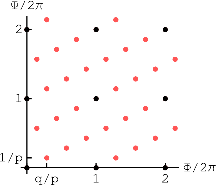
Note that identical points same as the origin induced by the identifications (87) and (88) are described as
| (89) |
where and are integers. If and are coprime natural numbers, there is no identical point same as the origin along the finite line connected with the origin and the point (89). The area of a unit lens space whose local metric is given by (86) becomes
| (90) |
Appendix B Regularity condition on the bolt
In this section, we study the regularity condition on the bolt off the black hole, i.e., and . The metric of four-dimensional Kerr-Taub-bolt space (4) diverges at apparently. These points correspond to fixed points of the Killing vector field . We expand the metric (2) near these fixed points, and obtain regularity conditions of identifications.
Introducing new coordinates,
| (95) |
near , the metric (2) behaves as
| (96) | |||||
The induced metric on the two-dimensional bolt is given by the second and the third terms in the second line of the above metric. The function takes larger value in the north part than the south part, so the shape of the bolt is like a pear. In fact, this asymmetric behavior leads a difference of topologies of each black holes.
Near the bolt , the metric (96) with takes the form
| (97) |
The above two-dimensional metric is regular if and only if the coordinate is periodic with a period along in plane. Equivalently, such the condition is same as the following identification
| (98) |
Using the coordinates (20), we see that the regularity condition (98) coincides with the condition (26).
References
- [1] P. Dobiasch and D. Maison, Gen. Rel. Grav. 14, 231 (1982).
- [2] G. W. Gibbons and D. L. Wiltshire, Annals Phys. 167, 201 (1986) [Erratum-ibid. 176, 393 (1987)].
- [3] J. P. Gauntlett, J. B. Gutowski, C. M. Hull, S. Pakis and H. S. Reall, Class. Quant. Grav. 20, 4587 (2003) [arXiv:hep-th/0209114].
- [4] D. Gaiotto, A. Strominger, X. Yin, JHEP 0602, 024 (2006). [hep-th/0503217].
- [5] H. Ishihara and K. Matsuno, Prog. Theor. Phys. 116, 417 (2006) [arXiv:hep-th/0510094].
- [6] H. Ishihara, M. Kimura, K. Matsuno and S. Tomizawa, Class. Quant. Grav. 23, 6919 (2006) [arXiv:hep-th/0605030].
- [7] K. Matsuno, H. Ishihara, T. Nakagawa and S. Tomizawa, Phys. Rev. D 78, 064016 (2008) [arXiv:0806.3316 [hep-th]].
- [8] Y. Chen and E. Teo, Nucl. Phys. B 850, 253 (2011) [arXiv:1011.6464 [hep-th]].
- [9] P. G. Nedkova and S. S. Yazadjiev, Phys. Rev. D 84, 124040 (2011) [arXiv:1109.2838 [hep-th]].
- [10] T. Tatsuoka, H. Ishihara, M. Kimura and K. Matsuno, Phys. Rev. D 85, 044006 (2012) [arXiv:1110.6731 [hep-th]].
- [11] K. Matsuno, H. Ishihara, M. Kimura and T. Tatsuoka, Phys. Rev. D 86, 104054 (2012) [arXiv:1208.5536 [hep-th]].
- [12] S. Tomizawa and S. ’y. Mizoguchi, Phys. Rev. D 87, 024027 (2013) [arXiv:1210.6723 [hep-th]].
- [13] C. Stelea, C. Dariescu and M. A. Dariescu, Phys. Rev. D 87, 024039 (2013) [arXiv:1211.3154 [gr-qc]].
- [14] Y. Kanou, H. Ishihara, M. Kimura, K. Matsuno and T. Tatsuoka, Phys. Rev. D 90, 084004 (2014) [arXiv:1408.2956 [hep-th]].
- [15] S. Tomizawa and H. Ishihara, Prog. Theor. Phys. Suppl. 189, 7 (2011) [arXiv:1104.1468 [hep-th]].
- [16] S. D. Majumdar, Phys. Rev. 72, 390 (1947).
- [17] A. Papapetrou, Proc. R. Ir. Acad. Sect. A 51, 191 (1947).
- [18] R. C. Myers, Phys. Rev. D 35, 455 (1987).
- [19] J. P. Gauntlett, R. C. Myers and P. K. Townsend, Class. Quant. Grav. 16, 1 (1999) [hep-th/9810204].
- [20] H. Ishihara, M. Kimura, K. Matsuno and S. Tomizawa, Phys. Rev. D 74, 047501 (2006) [hep-th/0607035].
- [21] H. Ishihara, M. Kimura and S. Tomizawa, Class. Quant. Grav. 23, L89 (2006) [hep-th/0609165].
- [22] K. Matsuno, H. Ishihara, M. Kimura and S. Tomizawa, Phys. Rev. D 76, 104037 (2007) [arXiv:0707.1757 [hep-th]].
- [23] K. -i. Maeda, N. Ohta, M. Tanabe, Phys. Rev. D74, 104002 (2006). [hep-th/0607084].
- [24] G. W. Gibbons and M. J. Perry, Phys. Rev. D 22, 313 (1980).
- [25] J. Kunz and S. Yazadjiev, Phys. Rev. D 79, 024010 (2009) [arXiv:0811.0730 [hep-th]].
- [26] J. Kunz, P. G. Nedkova and C. Stelea, Nucl. Phys. B 874, 773 (2013) [arXiv:1304.7020 [gr-qc]].
- [27] A. M. Ghezelbash, R. B. Mann and R. D. Sorkin, Nucl. Phys. B 775, 95 (2007) [hep-th/0703030].
- [28] Y. Chen and E. Teo, Nucl. Phys. B 838, 207 (2010) [arXiv:1004.2750 [gr-qc]].
- [29] H. K. Kunduri and J. Lucietti, Phys. Rev. Lett. 113, 211101 (2014) [arXiv:1408.6083 [hep-th]].
- [30] G. W. Gibbons, G. T. Horowitz and P. K. Townsend, Class. Quant. Grav. 12, 297 (1995) [hep-th/9410073].
- [31] D. L. Welch, Phys. Rev. D 52, 985 (1995) [arXiv:hep-th/9502146].
- [32] G. N. Candlish and H. S. Reall, Class. Quant. Grav. 24, 6025 (2007) [arXiv:0707.4420 [gr-qc]].
- [33] G. N. Candlish, Class. Quant. Grav. 27, 065005 (2010) [arXiv:0904.3885 [hep-th]].
- [34] C. N. Gowdigere, A. Kumar, H. Raj and Y. K. Srivastava, arXiv:1401.5189 [hep-th].
- [35] C. N. Gowdigere, arXiv:1407.5338 [hep-th].
- [36] M. Kimura, H. Ishihara, K. Matsuno and T. Tanaka, Class. Quant. Grav. 32, 015005 (2015) [arXiv:1407.6224 [gr-qc]].
- [37] M. Kimura, Phys. Rev. D 78, 047504 (2008) [arXiv:0805.1125 [gr-qc]].
- [38] C. M. Yoo, H. Ishihara, M. Kimura, K. Matsuno and S. Tomizawa, Class. Quant. Grav. 25, 095017 (2008) [arXiv:0708.0708 [gr-qc]].
- [39] M. Kimura, H. Ishihara, S. Tomizawa and C. M. Yoo, Phys. Rev. D 80, 064030 (2009) [arXiv:0906.4681 [gr-qc]].