Thermopower and Entropy: lessons from Sr2RuO4
Abstract
We calculate the in-plane Seebeck coefficient of Sr2RuO4 within a framework combining electronic structure and dynamical mean-field theory. We show that its temperature-dependence is consistent with entropic considerations embodied in the Kelvin formula, and that it provides a meaningful probe of the crossover out of the Fermi liquid regime into an incoherent metal. This crossover proceeds in two stages: the entropy of spin degrees of freedom is released around room-temperature while orbital degrees of freedom remain quenched up to much higher temperatures. This is confirmed by a direct calculation of the corresponding susceptibilities, and is a hallmark of ‘Hund’s metals’. We also calculate the c-axis thermopower, and predict that it exceeds substantially the in-plane one at high-temperature, a peculiar behaviour which originates from an interlayer ’hole-filtering’ mechanism.
pacs
71.27.+a,72.15.Jf,72.15.QmWhen a thermal gradient is established in a material, an electric field is also generated. This thermoelectric effect can be used for solid-state refrigeration and waste-heat recovery. The Seebeck coefficient (or thermopower) is the ratio , measured under the condition that no electrical current flows. It not only determines the suitability of the material for thermoelectric applications, but is also a useful fundamental characterization of its electronic state. In metals with strong electronic correlations, the slope of the thermopower at low temperature has been shown to scale with the linear coefficient of the specific heat [1]. This is an example of often noted but poorly understood relation between the thermopower and the entropy . A precise relation has been established only for a free electron gas at low temperature, in which case, [1] , and in the high-temperature atomic limit where the Heikes formula applies [1, 2]. This formula has been used to interpret the saturation of the thermopower at high-temperature in several transition-metal oxides [3, 5, 6]. More recently, it was suggested [7, 8] that the ‘Kelvin formula’ is a good approximation to the thermopower.
Here we consider ruthenates, especially Sr2RuO4 . We show that the thermopower provides key insights into the degrees of freedom which are relevant to the physics of these materials, and clarify when and how entropic considerations apply. Sr2RuO4 is arguably the cleanest and best documented among strongly correlated oxides, with extensive studies of its low-temperature Fermi liquid (FL) behavior [9] and unconventional superconductivity [10]. Recent work shifted the focus to properties at higher temperature and energy. It was shown that the low value of the scale K [11] below which Fermi liquid behaviour is observed, and the large effective mass enhancement, are due to the Hund’s rule coupling [5]. Ruthenates belong to a broader class of compounds that notably includes iron pnictides and have been called ‘Hund’s metals’ [13, 14, 15] (for a review, see [16]). Quasiparticle excitations, as revealed by a well-defined spectral function peak, were shown to persist well above , and the changes in the dispersion of these resilient quasiparticles [17] as a function of temperature [18] and frequency [19] explain the deviations from Fermi liquid behavior. Overall, these results suggest that one can characterize the crossover into the incoherent regime better than previously imaginable.
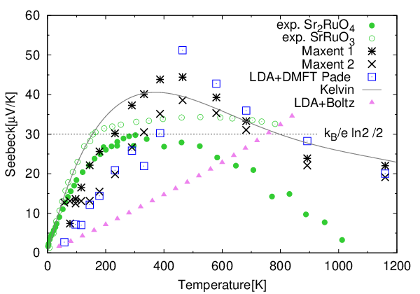
The ab-plane thermopower of ruthenates initialy increases linearly with , as expected in a FL, and saturates for K at a value of order - V/K (see Fig. 1 for Sr2RuO4 and SrRuO3). As noted in Refs. [5, 20, 21], this value depends weakly on the cation, the lattice structure and the doping. This universality is intriguing: does the value of thermopower reflect the active degrees of freedom in the metallic state above and thereby reveal its physical nature ? Boldly neglecting configurational and orbital contributions to the Heikes formula, the authors of Ref. [5] proposed that only spin degrees of freedom must be retained in the atomic entropy. May atomic considerations apply to an itinerant metal, and if so what happened to the neglected degrees of freedom ?
In this letter, we use electronic structure and dynamical mean-field theory (LDA+DMFT) to perform materials-realistic calculations of the thermopower of Sr2RuO4 based on the Kubo transport formalism. We show that the observed value of the room-temperature thermopower is explained by the fact that the spin degrees of freedom are fluctuating in this range of temperature, while the orbital moments remain quenched up to K. At this temperature, the thermopower displays a downturn, indicating that the decoherence proceeds via two distinct stages, a hallmark of Hund’s metals. We find that the in-plane thermopower is well approximated by the Kelvin formula for all temperatures, establishing a connection to entropic considerations. We also calculate the c-axis thermopower and predict a strong enhancement at high temperatures, which we explain by a hole-filtering mechanism resulting from the crystal structure of Sr2RuO4 .

We use the LDA+DMFT method, in the implementation of Refs. [25, 4, 27], as applied to Sr2RuO4 in earlier work [5, 19]. The rotationally invariant interaction was applied to the atomic shell, with and the total spin and orbital pseudo-spin operators, respectively. The same interaction parameters eV and eV as in Refs. [5, 19] were used. The thermopower in DMFT is , where is the Fermi function, , and the transport function reads:
| (1) |
Here, is a normalization volume, the spectral function matrix, and the band velocities in the -direction (in-plane response) or -direction (out of plane). Self-energies obtained by a continuous-time Monte-Carlo impurity solver [28, 27] were analytically continued using both a stochastic maximum entropy method [29] and Padé approximants [30]. The total energies were calculated from charge self-consistent calculations as implemented in Ref. [4].
The calculated thermopower is shown on Fig. 1 (full squares with errorbars). It increases linearly with temperature, reaches a maximum close to 500 K and then slowly diminishes as the temperature is further increased. Overall, the theoretical values agree reasonably well with experimental data.Above room-temperature, our results exceed the experimental values, even when the systematic error due to analytical continuation is taken into account. (The estimation of the errorbars that are indicated on Fig. 1 is discussed in the supplemental material [30] in which the overall consistency with Pade continuation is also presented). Also displayed on Fig. 1 is the LDA-Boltzmann estimate [31]. As expected, the slope of at low- is then too small by a factor of about four, consistent with the mass renormalization due to correlations.
We now consider the Kelvin approximation that arises [7] if the slow (thermodynamic) instead of the fast (transport) limit is used in the evaluation of Onsager coefficients. Alternatively, it can be derived using a physical argument, requesting that the density gradient vanishes instead of the current i.e. , and using the Maxwell relation into . Note that in the high- limit where , the Kelvin expression coincides with the Heikes formula , but that it has a greater degree of generality and can be investigated at any temperature. As shown on Fig 1, the Kelvin expression (obtained from a numerical derivative of the LDA+DMFT chemical potential 11 1 A polynomial interpolation has been used to perform the numerical derivative , see Fig. 2c) agrees with the Kubo result remarkably well. This finding extends to a real material the good agreement previously noted in model calculations [7, 17, 33].


The success of the Kelvin approximation hints at an entropic interpretation of the thermopower. In order to identify which degrees of freedom are active at a given temperature, we calculated the local spin and orbital susceptibilities, displayed on Fig. 2 (a,b) as a function of temperature and frequency. The spin susceptibility has a Curie-like behaviour, indicating fluctuating spin moments which are quenched only below the very low scale [5], which can be interpreted in DMFT as the Kondo temperature associated with the atomic shell coupled to its environment. Orbital susceptibilities behave in a drastically different manner. They are much smaller than the magnetic one for K, and weakly dependent on temperature up to K. Above this temperature, they start to increase, indicating the gradual un-quenching of orbital degrees of freedom. At low temperature the frequency dependence of spin- and orbital susceptibilities are drastically different. The latter shows an activated behavior with a peak at about eV, that likely comes from transitions from to states, corresponding to an energy difference . At high temperature, this distinction between spin and orbital susceptibilities disappears.
We also estimated the temperature dependence of the entropy. To this aim, we calculated the LDA+DMFT total energy as a function of , displayed in Fig. 2(c) and used the thermodynamic relation (see supplemental material [30]) to estimate the entropy. It is seen (Fig. 2(d)) that the entropy corresponding to unquenched spins for Ru4+ (spin-, ) is reached by room temperature, while the entropy corresponding to both unquenched spins and orbitals (spin-, , ) is reached at much higher K.
These findings that reveal that the decoherence proceeds in two stages, in which the orbital entropy is released only after the spins are fully liberated, reinforce the Hund’s metal picture of Sr2RuO4 . They are in line with the analytical study of Refs [34, 35], in which a quantum impurity model appropriate to these systems was considered. This model involves three Kondo-like coupling constants, corresponding to spin-only, orbital-only and mixed spin-orbital degrees of freedom. It was found that the spin coupling is much smaller than the other two, and can even be ferromagnetic, so that the screening of orbital degrees of freedom occurs at higher temperature, while that of the spin degrees of freedom is controlled by the growth of the spin-orbital coupling and occurs at a lower temperature. Incidentally, the quenching of orbital moments at high- may explain why calculations neglecting the spin-orbit coupling [5, 19] may still be accurate for ruthenates down to quite low , even though the bare value of this coupling is eV [36].
Having identified the relevant degrees of freedom, we can now give an interpretation of the thermopower in terms of a simple Heikes-like estimate [1, 2]. This was previously attempted in Ref. [5] which considered an intermediate valence , mixing Ru and Ru, for which: . The authors of Ref. [5] observed that the first term gives reasonable values for the thermopower provided only spin degrees of freedom are retained in evaluating the degeneracies , i.e. with for , and , respectively (in agreement with Hund’s rule). The problem with this reasoning is that the second term, corresponding to configurational entropy, is neglected and would otherwise yield a diverging result on approaching the actual valence () of Sr2RuO4 . We thus reconsider the Heikes analysis for this integer valence and obtain, by considering the high- limit of the chemical potential (see supplemental material for derivation [30]): V/K. This expression differs from the previous one on several counts. Importantly, the problematic configurational term does not appear. Furthermore it involves only the degeneracies of the two neighbouring configurations and (note also the factor in front of the logarithm). The estimated value V/K agrees reasonably with the observed one in the room-temperature plateau regime, and points to the heart of the Hund’s coupling dominated nature of ruthenates: fluctuating spins and quenched orbital moments. Keeping orbital degrees of freedom and full degeneracies (spin-,), (spin , ) would instead yield a negative value V/K. Indeed decreases at higher , although this negative value is not reached in our calculation perhaps because other atomic multiplets become relevant, which are not included in the description.

Although the agreement between the in-plane thermopower and the entropic Kelvin formula is remarkable, one has to keep in mind that this formula is only approximate and derived in a way that largely ignores the transport nature of thermoelectric coefficients. For instance, in a non-cubic system, these coefficients can be different along different crystal axis, as recently discussed for organic conductors in Ref. [37]. It was pointed out there (see also [8]) that the Kelvin formula, which includes no information about current matrix elements, obviously cannot account for such an anisotropy. We have calculated the c-axis thermopower of Sr2RuO4 , and found a striking manifestation of this effect. As reported on Fig. 3, the c-axis thermopower behaves differently from both the in-plane one and from the Kelvin approximation above room-temperature. It becomes remarkably large for a metallic system, reaching V/K at K. Since, to our knowledge, the c-axis thermopower has not yet been measured for Sr2RuO4 , this finding is a prediction for future experiments.
To get basic insight into when the Kelvin formula can be expected to work, it is instructive [8] to consider a non-interacting system in which with the density-of-states. The expression of the thermopower has the same form, with the important difference that the transport function along the appropriate axis replaces . Hence, the Kelvin formula is expected to be a good approximation only when the transport function has a similar energy-dependence as the density of states.
In Fig. 4 we display the LDA+DMFT (a) and the LDA(b) transport functions. In contrast to the in-plane one, the c-axis transport function exhibits a pronounced peak at negative energies ( eV in LDA, renormalized down to eV in LDA+DMFT). The LDA density-of-states (dashed) has a three-peak structure, with the outer two peaks originating from the quasi 1d xz/yz bands. The c-axis transport function exhibits a pronounced negative frequency peak only and is thus characterized by a strong asymmetry favouring holes. This occurs because, as illustrated on panels (b,c) of Fig. 4, the dispersion of the bands as a function of is much stronger close to the center of the Brillouin zone, which corresponds to occupied states below Fermi level. The large c-axis thermopower is thus due to an interlayer ‘hole-filtering’ mechanism. The origin of such a behavior can be traced to the body centered crystal structure, in which the main hopping along the c-direction proceeds via the central atom. In a tight-binding picture, this gives rise to a band energy of the form and the corresponding velocities in the direction are indeed maximal at the zone center where the much larger in-plane term (counted from Fermi level) is strongly negative. The effect is largest when the thermal width of the function becomes comparable to the energy of the peak in the LDA+DMFT spectral function: eV, i.e at temperatures K.

In summary, we have shown that the thermopower of ruthenates carries key physical information, and indicates in particular that the decoherence temperature at which the corresponding entropy is unquenched is much smaller for spin than for orbital degrees of freedom, a characteristic signature of a Hund’s metal. Our calculations also predict a different behaviour and a large value of the c-axis thermopower at high temperature, which results from an interlayer ‘hole-filtering’ inherent to the crystal structure of Sr2RuO4 . In contrast to the in-plane results, this illustrates the limitation of entropic interpretations of the thermopower. That entropy limitations can be overcome may be good news for applications, and it would be worth exploring whether such hole-filtering can be found and exploited in thermoelectric materials.
Acknowledgements.
We acknowledge useful discussions with K. Behnia, R. Daou, F. Gascoin, S. Hébert, J. Kokalj, G. Kotliar, A. Maignan, S. Shastry, L. Taillefer, and the contribution of Xiaoyu Deng in the development of the transport code. This work was supported by the Slovenian Research Agency (ARRS) under Program P1-0044, by the European Research Council (ERC-319286 QMAC), and by the Swiss National Science Foundation (NCCR MARVEL).References
- [1] K. Behnia, D. Jaccard, and J. Flouquet, J. Phys.: Condens. Matter 16, 5187 (2004).
- [2] P. M. Chaikin and G. Beni, Phys. Rev. B 13, 647 (1976).
- [3] J.-P. Doumerc, Journal of Solid State Chemistry 109, 419 (1994).
- [4] W. Koshibae, K. Tsutsui, and S. Maekawa, Phys. Rev. B 62, 6869 (2000).
- [5] Y. Klein, S. Hébert, A. Maignan, S. Kolesnik, T. Maxwell, and B. Dabrowski, Phys. Rev. B 73, 052412 (2006).
- [6] M. Uchida, K. Oishi, M. Matsuo, W. Koshibae, Y. Onose, M. Mori, J. Fujioka, S. Miyasaka, S. Maekawa, and Y. Tokura, Phys. Rev. B 83, 165127 (2011).
- [7] M. R. Peterson and B. S. Shastry, Phys. Rev. B 82, 195105 (2010).
- [8] T. W. Silk, I. Terasaki, T. Fujii, and A. J. Schofield, Phys. Rev. B 79, 134527 (2009).
- [9] C. Bergemann et al., Adv. Phys. 52, 639 (2003).
- [10] A. P. Mackenzie and Y. Maeno, Rev. Mod. Phys. 75, 657 (2003).
- [11] N. E. Hussey, A. P. Mackenzie, J. R. Cooper, Y. Maeno, S. Nishizaki, and T. Fujita, Phys. Rev. B 57, 5505 (1998).
- [12] J. Mravlje, M. Aichhorn, T. Miyake, K. Haule, G. Kotliar, and A. Georges, Phys. Rev. Lett. 106, 096401 (2011).
- [13] P. Werner, E. Gull, M. Troyer, and A. J. Millis, Phys. Rev. Lett. 101, 166405 (2008).
- [14] K. Haule and G. Kotliar, New J. Phys. 11, 025021 (2009).
- [15] Z. P. Yin, K. Haule, and G. Kotliar, Nat. Mater. 10, 932 (2011).
- [16] A. Georges, L. de‘Medici, and J. Mravlje, Annu. Rev. Cond. Matt. Phys. 4, 137 (2013).
- [17] X. Deng, J. Mravlje, R. Žitko, M. Ferrero, G. Kotliar, and A. Georges, Phys. Rev. Lett. 110, 086401 (2013).
- [18] W. Xu, K. Haule, and G. Kotliar, Phys. Rev. Lett. 111, 036401 (2013).
- [19] D. Stricker, J. Mravlje, C. Berthod, R. Fittipaldi, A. Vecchione, A. Georges, and D. van der Marel, Phys. Rev. Lett. 113, 087404 (2014).
- [20] Y. Klein, Crucial role of the orbital and spin degeneracies in the thermoelectric power of metallic oxides, Ph.D. thesis, Universite de Caen (2006).
- [21] S. Hébert, R. Daou, and A. Maignan, Phys. Rev. B 91, 045106 (2015).
- [22] H. Yoshino, K. Murata, N. Shirakawa, Y. Nishihara, Y. Maeno, and T. Fujita, Journal of the Physical Society of Japan 65, 1548 (1996).
- [23] X. F. Xu, Z. A. Xu, T. J. Liu, D. Fobes, Z. Q. Mao, J. L. Luo, and Y. Liu, Phys. Rev. Lett. 101, 057002 (2008).
- [24] N. Keawprak, R. Tu, and T. Goto, Materials Transactions 49, 600 (2008).
- [25] M. Aichhorn, L. Pourovskii, V. Vildosola, M. Ferrero, O. Parcollet, T. Miyake, A. Georges, and S. Biermann, Phys. Rev. B 80, 085101 (2009).
- [26] M. Aichhorn, L. Pourovskii, and A. Georges, Phys. Rev. B 84, 054529 (2011).
- [27] M. Ferrero and O. Parcollet, TRIQS: A Toolbox for Research on Interacting Quantum Systems, http://ipht.cea.fr/triqs.
- [28] E. Gull, A. J. Millis, A. I. Lichtenstein, A. N. Rubtsov, M. Troyer, and P. Werner, Rev. Mod. Phys. 83, 349 (2011).
- [29] K. S. D. Beach, ArXiv:cond-mat/0403055.
- [30] See Supplemental Material.
- [31] G. Madsen and D. Singh, Comp. Phys. Comm. 175, 6771 (2006).
- [32] A polynomial interpolation has been used to perform the numerical derivative , see Fig. 2c.
- [33] L.-F. Arsenault, B. S. Shastry, P. Sémon, and A.-M. S. Tremblay, Phys. Rev. B 87, 035126 (2013).
- [34] Z. P. Yin, K. Haule, and G. Kotliar, Phys. Rev. B 86, 195141 (2012).
- [35] C. Aron and G. Kotliar, Phys. Rev. B 91, 041110 (2015).
- [36] M. W. Haverkort, I. S. Elfimov, L. H. Tjeng, G. A. Sawatzky, and A. Damascelli, Phys. Rev. Lett. 101, 026406 (2008).
- [37] J. Kokalj and R. H. McKenzie, Phys. Rev. B 91, 125143 (2015).
Supplemental Material
to
Thermopower and entropy: lessons from Sr2RuO4
J. Mravlje1 and A. Georges,2,3,4
1Jožef Stefan Institute, Jamova 39, 1000 Ljubljana, Slovenia
2Collège de France, 11 place Marcelin Berthelot, 75005 Paris, France
3Centre de Physique Théorique, École Polytechnique, CNRS, 91128
Palaiseau, France
4DQMP, Université de Genève, 24 quai Ernest Ansermet, CH-1211 Genève, Suisse
Supplementary Material
for
Thermopower and Entropy: lessons from Sr2RuO4
I Generalized Heikes formula for integer occupancies in multiorbital systems
The Heikes formula [1] approximates the Seebeck coefficient as
| (2) |
In this expression, is the chemical potential and indicates that is to be evaluated in the atomic limit. It is actually simpler to consider directly (instead of evaluating it via the thermodynamic relation and evaluating the entropy from the number of possible configurations, as originally done in Ref. [1]).
If the average occupancy is non-integer (for integer), in the atomic limit is controlled by the degeneracies of the atomic state with and electrons, and all other valence states can be neglected. The occupancy is given by:
| (3) |
in which is the degeneracy of the atomic state with electrons and its energy. Solving this equation for reads:
| (4) |
From this expression, it is clear that reaches a finite value in the high-temperature limit (hence that ) and that the term involving provides only a subleading correction. As a result, one obtains:
| (5) |
which is the Heikes formula appropriate for fractional occupancy , as generalized to account for atomic degeneracies in Refs. [2, 3]
For integer occupancy , the above calculation must be modified since both neighboring valence states must be retained, as well as of course itself. The expression of now reads:
| (6) |
Solving for and neglecting as above the subdominant corrections in now leads to the simple expression:
| (7) |
We note that this generalization of the Heikes expression appropriate to integer valence does not involve the configurational entropy term, but only the degeneracies of the atomic states with neighboring valence .
II Analytically continued self energies and comparison to Padé


The analytical continuation of imaginary frequency data remains challenging even with the most recent fast and accurate quantum impurity solvers based in continuous time Quantum Monte-Carlo. For the data shown in the main text we used the self energies obtained using stochastic Maximum Entropy approach. In practice, we analytically continue auxiliary Green’s function for a constant and extract the self energy by inverting the resulting . To estimate the error of our procedure, we set to two different values (that should give identical answer for ideal analytical continuation procedure on noiseless data): (1) the real part of the Matsubara self energy at the lowest Matsubara frequency (2) the double counting correction , where is the occupancy of the shell. The two values of are close, the former being about 0.2eV larger than the latter. As an independent crosscheck, we analytically continued the self energies also directly using Padé approximants.
The real frequency self energies for selected temperatures are presented in Fig. SM1. One sees that the two choice of (denoted by Maxent 1 and 2, respectively) give very similar results. The data agrees quite well also with the self energies obtained with Padé, in particular for energy .
On Fig.SM2 we show the calculated Seebeck coefficients using as an input the different real frequency self energies just discussed (stars, crosses and squares for the two choices of and Padé, respectively). Whereas quantitatively the differences are certainly not negligible, as the calculation of the Seebeck coefficient is very sensitive to the low energy particle-hole asymmetry of the imaginary part of the self energy, that is particularly difficult to extract accurately, all the data gives similar temperature dependence, with a maximum at about 450K.
Overall, the maximum entropy calculations agrees well with Padé result. Near 450K, however, the Padé data displays an abrupt jump. The origin of this jump can be traced to abrupt shift of the minimum of towards the negative frequency side in the Padé data. The shift of the minimum that occurs at the a temperature where the orbital moments start unquenching (see main text), which causes the maximum in the Seebeck coefficient occurs in the Maximum Entropy data in a milder continuous fashion (see Fig. SM3). Padé approximants are unable to fit the self energy through the crossover, hence discontinous jump.
For the main text we used an average of the two stochastic maxent runs in the calculation of Seebeck coefficient and the difference between the two results was used as an indicative error bar.

III Calculation of total energy and entropy
The total energy is calculated from the charge self-consistent LDA+DMFT calculation, as described in Ref. [4]. The value of the energy and the errorbars on the plot in the main text were obtained from the variance of the total energy in 20 consecutive iterations of a charge self-consistent LDA+DMFT loop, starting from a converged solution.
The precision of our data is not sufficient to obtain the entropy by direct integration of the thermodynamic relation
| (8) |
hence we estimate the entropy in an aproximate way. At low-, the temperature dependence of the energy follows a Fermi-liquid form , with mJ/molK2 for Sr2RuO4 . (Mass renormalization found in experiment is consistent with the one found in LDA+DMFT [5]). At higher , the energy is found to depend approximately linearly on temperature. Hence, we used a fit for and for , with such that is continuous. We find and K. The entropy is then obtained by integrating the thermodynamic relation Eq. 8, which yields for and for . This estimate of the entropy is displayed on Fig. 2(d) of the main text.
References
- [1] P. M. Chaikin and G. Beni, Phys. Rev. B 13, 647 (1976).
- [2] J.-P. Doumerc, Journal of Solid State Chemistry 109, 419 (1994).
- [3] W. Koshibae, K. Tsutsui, and S. Maekawa, Phys. Rev. B 62, 6869 (2000).
- [4] M. Aichhorn, L. Pourovskii, and A. Georges, Phys. Rev. B 84, 054529 (2011).
- [5] J. Mravlje, M. Aichhorn, T. Miyake, K. Haule, G. Kotliar, and A. Georges, Phys. Rev. Lett. 106, 096401 (2011).