Quantitative Analysis of Probabilistic Models of Software Product Lines with Statistical Model Checking
Abstract
We investigate the suitability of statistical model checking techniques for analysing quantitative properties of software product line models with probabilistic aspects. For this purpose, we enrich the feature-oriented language FLan with action rates, which specify the likelihood of exhibiting particular behaviour or of installing features at a specific moment or in a specific order. The enriched language (called PFLan) allows us to specify models of software product lines with probabilistic configurations and behaviour, e.g. by considering a PFLan semantics based on discrete-time Markov chains. The Maude implementation of PFLan is combined with the distributed statistical model checker MultiVeStA to perform quantitative analyses of a simple product line case study. The presented analyses include the likelihood of certain behaviour of interest (e.g. product malfunctioning) and the expected average cost of products.
1 Introduction
The modelling and analysis by means of process calculi and formal verification techniques like model checking of the variety of configurations and behaviour that is common to a software product line (SPL) is gaining momentum [24, 8, 7, 17, 19, 18, 10, 9, 34, 39, 40, 6]. Compared to the complexity of verifying the behaviour of a single product or a single system, the variability inherent to SPL adds another dimension as the number of possible products of an SPL may be exponential in the number of features [12]. In [7], we introduced the feature-oriented language FLan as a high-level modelling language for SPLs. A rich set of process-algebraic operators allows one to specify in a procedural, operational way both the configuration and the behaviour of products, while a constraint store allows one to specify in a declarative way all common structural constraints known from feature models and additional action constraints typical of feature-oriented software development. On the one hand, the execution of a process is constrained by the store (e.g. to avoid introducing inconsistencies), while on the other hand a process can query the store (e.g. to resolve configuration options) or update the store (e.g. to add new features, also at run time or by means of a staged configuration process). An implementation of FLan in the executable modelling language Maude [20] allows one to exploit Maude’s rich toolkit for a variety of formal analyses of FLan models, ranging from consistency checking (by means of SAT solving) to model checking.
In this paper, we introduce a probabilistic extension of FLan: PFLan allows to equip actions with rates to specify probabilistic SPL models (e.g. to model uncertainty, failure rates, randomisation). This paves the way for quantitative analyses (e.g. to measure quality of service, reliability, performance). Here we present a proof-of-concept use of an implementation of PFLan in Maude in combination with the distributed statistical model checker MultiVeStA [37] to estimate the likelihood of specific behaviour. Formally, our approach is to perform a sufficient number of probabilistic simulations of a PFLan model to obtain statistical evidence (with a desired level of statistical confidence) of quantitative properties under scrutiny. The properties are formulated in MultiVeStA’s property specification language MultiQuaTEx, which allows to express and evaluate more than one property over the same simulated path (behaviour) [37]. The advantage over exhaustive (probabilistic) model checking is that there is no need to generate entire state spaces. We argue that this outweighs the main disadvantage of having to give up on obtaining exact results (100% confidence) with exact analysis techniques like probabilistic model checking, in particular when examining an SPL, given their possibly exponential number of products.
We refer to [4] for (probabilistic) model checking and to [30, 29] for statistical model checking. An overview of related work on applying formal analysis techniques in SPLE can be found in [39], while [7] contains an extensive discussion of related work on model-checking SPL behaviour. As far as we know, there are only a few, quite different, approaches on probabilistic model checking of an SPL [25, 41, 23], whereas we present here the first application of statistical model checking in SPL engineering (SPLE).
The paper outline is as follows. Section 2 contains a toy example of a product line of coffee machines, adapted from [6, 7, 8, 10, 9]. Section 3 presents PFLan, followed by a PFLan model of the example in Section 4. MultiVeStA is introduced in Section 5, followed by experimental quantitative analyses of the example in Section 6. Section 7 summarises the contributions of this paper and discusses future work.
2 An Example Product Line of Coffee Machines
Our toy example is a (simplistic) product line of coffee machines with the following list of requirements:
- 1.
Initially, a coin must be inserted: either a euro, exclusively for products for the European market, or a dollar, exclusively for Canadian products;
- 2.
An optional cancel button allows the user to cancel coin insertion, after which the coin is returned;
- 3.
A machine that contains a coin must offer a choice to add sugar, followed by a choice of beverages;
- 4.
The choice of drinks (coffee, tea, cappuccino) varies, but all products must offer at least one drink, tea may be offered only by European products, and products offering cappuccino must offer coffee;
- 5.
An optional ringtone may be rung after beverage delivery. It must be rung after serving cappuccino;
- 6.
After the drink is taken, the machine returns idle.
These requirements for products combine structural constraints defining valid feature configurations (e.g. “every product must offer at least one beverage”) with temporal constraints defining valid product behaviour in terms of valid action sequences (e.g. “a ringtone must be rung after serving a cappuccino”).
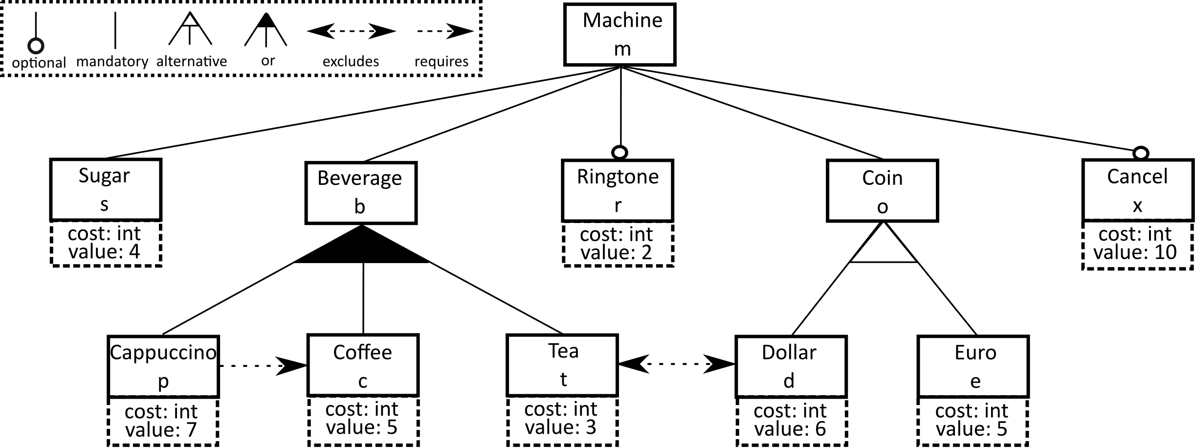
The de facto standard variability model in SPLE is a feature model [28, 35]. It provides a compact representation of all valid products of a product line in terms of their features (behaviour is not captured). An (attributed) feature model of our example is depicted in Fig. 1. It has a root (feature) and a set of non-trivial features, partitioned into the sets of compound features and of primitive features.11 1 In case no confusion can arise, we often simply speak of features when we actually refer to the primitive features. The only purpose of the former is to group the (primitive) features in the tree, whereas the latter define user observable configuration parameters [5, 35]. We identify a product from the product line with a non-empty subset of Features. Deciding whether a product satisfies a feature model can be reduced to Boolean satisfiability (SAT), and efficiently be computed with SAT solvers [5].
By equipping features with (non-functional) attributes (e.g. ) we obtain an attributed feature model.22 2 Additional quantitative constraints on (combinations of) features may be defined (e.g. ) but we prefer to neglect them in this paper, as such constraints require the use of SMT solvers like Microsoft’s Z3 [31], currently under integration in our framework. The cost function , associated to the attribute , straightforwardly extends to products: . Thus, intuitively, can be seen as a labelling function assigning a non-negative integer to each product defined by a feature model.
3 PFLan: Syntax and Semantics
The feature-oriented language PFLan is a probabilistic extension of FLan [7], a process algebra that neatly separates declarative (pre-)configuration from procedural run-time aspects. PFLan is inspired by the concurrent constraint programming paradigm of [33], its adoption in process calculi [15] and its stochastic extension [13]. A constraint store allows one to specify all common constraints known from feature models in a declarative way, while a rich set of process-algebraic operators allow to specify the configuration and behaviour of product lines in a procedural way. The semantics smoothly unifies static (pre-configuration) and dynamic (run-time) feature selection.
The core notions of PFLan are features, constraints, processes (with action rates) and fragments, all visible in its syntax in Fig. 2. More precisely, and range over features while the syntactic categories , and correspond to fragments, a constraint store and processes (with actions from ), respectively.
The universe of (primitive) features is denoted by . The features of our example are the accepted coin slots (i.e. euro and dollar), the offered drinks (i.e. coffee, tea and cappuccino) and the additional capabilities sugar, cancel and ringtone (to add sugar, cancel coin insertion and ring a tone, respectively).
The declarative part of PFLan is represented by a store of constraints on features extracted from the product line requirements plus some additional information (e.g. about the context wherein the product will operate). Two important notions of a constraint store are the consistency of , denoted by (which in our case amounts to logical satisfiability of all constraints constituting ) and the entailment of constraint in (which in our case amounts to logical entailment). A constraint store contains any term generated by according to the syntax of PFLan. The most basic constraint stores are (no constraints at all), (inconsistent constraints) and ordinary Boolean propositions (generated by ). Constraints can be combined by juxtaposition (its semantics amounts to logical conjunction).
We assume that constraints on features are expressed using Boolean propositions (cf. [35]). Moreover, we assume that the universe of propositions contains a Boolean predicate that can be used to denote the presence of a feature in a product. Boolean propositions can also be used to represent additional information such as contextual facts. In our example we use the Boolean propositions and to state the fact that the coffee machine being configured is meant to be used in Europe or in Canada, respectively. Finally, Boolean propositions can state relations between contextual information and features, like (i.e. a coffee machine has a coin slot for euro’s only if it is intended for the European market).
Two common cross-tree constraints are instead handled as first-class citizens in PFLan. A constraint expresses that feature requires the presence of feature , whereas a constraint expresses that features and mutually exclude each other’s presence (i.e. they are incompatible). Also these constraints could of course be encoded as Boolean propositions (e.g. and can equivalently be expressed as and , respectively). We in fact use such logical encodings to reduce consistency checking and entailment to logical satisfiability (and hence exploit Maude’s SAT solver). However, we prefer to keep this first-class treatment as syntactic sugar. In our example, we extract to formalise that and are mutually exclusive features (requirement 1) and to formalise that requires (requirement 3).
We also consider a class of action constraints, reminiscent of featured transition systems (FTS) [19]. In an FTS, transitions are labelled with actions and with Boolean constraints over the set of features. We associate arbitrary constraints to actions rather than to transitions (and we moreover add a rate to the actions, discussed below). In a coffee machine offering coffee, e.g., we will use for the (user) action of choosing coffee and as a proposition stating the execution of that action. The relation between the action and the presence of the corresponding feature can be formalised as , i.e. the choice for coffee requires coffee being offered by the coffee machine. In general, we assume that each action may have a constraint , where is a proposition. Such constraints act as a kind of guards to allow or forbid the execution of actions (cf. the discussion of the rule Act below). Note that these action constraints could also be more complex, e.g. we could define an action -- together with the action constraint .
The procedural part of PFLan is represented by processes which can be of the following type:
-
the empty process that does nothing;
-
a process identifier;33 3 We assume there is a set of process definitions of the form and recursively defined processes to be finitely branching.
-
a process that can perform action with rate and then behaves as ;
-
a process that can non-deterministically choose to behave as either or ;
-
a process that must progress first as and then as ;
-
a process formed by the parallel composition of and , which evolve independently.
We distinguish ordinary actions from a universe and two special actions (which will be used to denote the dynamic installation of a feature ) and (which can used to query the store for the validity of a Boolean proposition from ). As we will see shortly, each action type is treated differently in the operational semantics. Note, moreover, that each action has an associated rate (sometimes called weight), which is used to determine the probability that this action is executed. As usual, the probability to execute an action in a certain state depends on the rates of all other actions enabled in the same state. We will illustrate this in our example in Section 4. We consider the actions , (respective coin insertion), (cancellation of coin insertion), (sugar selection), (ringtone emission), , and (beverage selection) in our example. Their associated rates are discussed below. For simplicity we consider only constant rates, but our framework can be easily extended to allow store-dependent rates (e.g. to be able to reflect a higher probability to order cappuccino in Europe).
Finally, a fragment is a term , composed by a constraint store and a process . These two components may influence each other according to the concurrent constraint programming paradigm [33]: a process may update its store which, in turn, may condition the execution of the process’ actions.
The operational semantics is formalised in terms of the state transition relation defined in Fig. 3, where denotes the set of all terms generated by in the grammar of Fig. 2. Note that multisets of transitions are needed to deal with the possibility of having multiple instances of a transition . Technically, such a reduction relation is defined in structural operational semantics (SOS) style (i.e. by induction on the structure of the terms denoting a fragment) modulo the structural congruence relation defined in Fig. 4. The reduction relation implicitly defines a labeled transition system LTS, whose labels are rates. It is straightforward to obtain a discrete time Markov chain (DTMC) from such LTSs by normalising the rates into such that in each state, the sum of the rates of its outgoing transitions equals one. As usual, in the resulting DTMC the label of a transition corresponds to the probability that such a transition is executed starting from its source state. Recall that we advocate the use of statistical model checking because in general the DTMC is too large to generate.
The rules Inst and Act of the semantics are very similar, both allowing a process to execute an action if certain constraints are satisfied. Rule Inst forbids inconsistencies caused by the introduction of new features. It can be seen as a particular instance of the rule for the tell operation of concurrent constraint programming [33] instantiated as . Rule Act forbids inconsistencies with respect to action constraints. A typical action constraint is , i.e. action is subject to the presence of feature . Rule Ask formalises the semantics of the operation from concurrent constraint programming [33]. It allows a process to be blocked until a proposition can be derived from the store. Rules Par, Seq and Or formalise interleaving parallel composition, sequential composition and non-deterministic choice, respectively. Note that the non-determinism introduced by choices and parallel composition is probabilistically resolved in the aforementioned DTMC semantics.
Summarising, we note a variety of ways in which a feature can be included in a configuration. First, an explicit and declarative way is to include the proposition in the initial store; this is the way to include core features. Second, an implicit and declarative way is to derive from other constraints (e.g. if a store contains and , then ’s presence follows). Third, a procedural way is to dynamically install at run time; this key aspect originating from FLan enables staged configuration as known from dynamic software product lines [22, 14]. Building on FLan, PFLan combines these three ways in an elegant and consistent manner. The introduction of action rates in PFLan moreover allows one to specify probabilistic aspects of SPL models such as the behaviour of the user of a product and the likelihood of installing a certain feature at a specific moment with respect to that of other features.
4 A PFLan Model of the Example Product Line
Fig. 5 shows a specification of the family of coffee machines in PFLan. Fragment is composed of store and a process . The latter specifies an initial configuration phase , during which all primitive features except can be installed (the order of installation is influenced by the relative weight of the features, more on this below). This phase ends at a certain moment when a specific product (coffee machine) is said to be pre-configured, modeled by the installation of an ad-hoc defined feature , thus initiating the execution of process , which specifies the product’s run-time behaviour. Note that it is specifically allowed to install (or bind) a feature at run time (cf. in our toy example).
The store, instead, is made up of two parts: constraints derived from the requirements () plus contextual information (). The current action constraints are quite simple (all are of the form ) but, as said before, they could be more sophisticated upon need (e.g. the constraint on action could be specified as to require not only the presence of its corresponding feature but also that of the feature). In Fig. 5, a product line of European coffee machines is instantiated by the explicit context information .
The configuration process is a simple rated choice among the installation of some of the features a coffee machine may exhibit. This specifies a sort of race between features and may be thought of as independent designers competing to install the features for which they are responsible. The semantics of PFLan ensures that all executions will result in a consistent configuration if the process begins with a consistent store, i.e. the semantics forbids the installation of features that are mutually exclusive or prohibited by (a combination of) the constraints. Formally, multiple installations of the same feature does not have any effect, as installed features are organised in a set. The rates of the actions influence this race by determining a higher (or lower) probability for the installation of one feature with respect to another (or prior to another). In our example, to reflect the fact that and are core features, we assign higher rates to them than to the optional features to raise their chances of being installed first. Moreover, since we are modelling a coffee machine and since coffee is a necessary ingredient for cappuccino, we assign a higher rate to the feature than to those of other drinks. As a result, the probability to install in the first step, given that also , , , , and can be installed, thus becomes .
Process , finally, describes the run-time execution of a coffee machine. The machine may either accept a euro or a dollar, depending on the market it is meant for. After that, the user may cancel coin insertion, upon which the machine returns to its initial state and (usually) returns the coin. With a probability of , however, the machine does not return the coin (viz. ). If coin insertion is not canceled, the user may () or may not () push a button for sugar. In case sugar is selected, it is also poured, after which the user can select a beverage. But, with a probability of the machine is out of sugar, after which the user may either cancel the coin insertion or go for an unsugared drink. Beverage selection (more likely coffee than tea or cappuccino) is followed by the drink being poured (again with a probability that the chosen drink is unavailable), which in case of cappuccino concerns both milk and coffee. In case coffee or tea was chosen but unavailable, the user can again choose a beverage (and the machine may have been refilled). In the specific case that milk was poured but coffee is not available, the user has bad luck as the machine returns to its idle state before completing the chosen beverage. In case a drink was poured successfully, a ringtone may follow (in which case it first needs to be installed). The user then either takes the drink or, with a probability, realizes that sadly enough there was no cup available. Either way, the machine returns to its initial state.
Note how the rates ‘influence’ the behavior, in the sense that the choice operator is no longer purely non-deterministic, but probabilistic, i.e. the rates provide a probabilistic model of the behavior of the coffee machine and its environment (the users). Consider, e.g., the choice of a beverage: . The probability to choose coffee is (viz. ), compared to for tea and for cappuccino. Similarly, the probability to cancel coin insertion is (i.e. rather low). Note that we need to expand processes and to calculate this probability.
The rates that we assigned in this example merely serve to illustrate the proof-of-concept that we present in this paper. In practice, those rates may be obtained from a statistical analysis of the actual product configuration processes and product behaviours, possibly contained in historical logs.
Note that and are not purely distinct (pre-)configuration and run-time processes, respectively: feature may be installed dynamically at run time (i.e. possibly by but never by ) and it can be thought of as, e.g., a software module. This is an example of a staged configuration process, in which some optional features are bound at run time rather than at (pre-)configuration time.
5 Quantitative Analysis with MultiVeStA
MultiVeStA [37] is a statistical analysis tool developed and maintained by S. Sebastio and A. Vandin. It extends the (distributed) statistical model-checking tools PVeStA [3] and VeStA [38], developed at the Department of Computer Science of the University of Illinois at Urbana-Champaign. Differently from its predecessors, MultiVeStA can easily be integrated with any formalism which allows for probabilistic simulations. It has so far been used to analyse transportation systems [26], volunteer clouds [36], crowd-steering [32] and swarm robotic [11] scenarios.
In this paper, we use MultiVeStA to analyse PFLan specifications in order to obtain statistical estimations of quantitative properties expressed in MultiVeStA’s query language MultiQuaTEx (an extension of QuaTEx [2]). MultiVeStA provides such estimations by means of distributed statistical analysis techniques known from statistical model checking [30, 29]. A prototypical tool integrating MultiVeStA and PFLan is available at https://code.google.com/p/multivesta/wiki/PFLan together with all files necessary to reproduce the experiments discussed in this section.
Probabilistic simulations of a PFLan specification can easily be obtained by executing the model step-by-step by applying the rules of Fig. 3, each time selecting one of the computed one-step next-states according to the probability distribution obtained after normalising the rates of the generated transitions. Classical statistical model checking techniques allow one to perform analyses like “is the probability that a property holds greater than ?” or “what is the probability that a property is satisfied?” over a given specification. Next to performing such kinds of analyses over products, MultiVeStA also allows to estimate the expected values of properties that can take on any value from , like “what is the average cost of products generated from a software product line specification?”. Estimations are computed as the mean value of samples obtained from simulations, with large enough to grant that the size of the confidence interval (CI) is bounded by . In other words, if a MultiQuaTEx expression is estimated as , then with probability its actual expected value belongs to the interval . A CI is thus specified in terms of two parameters: and . In all experiments discussed in this section, we fixed , and and for probabilities and costs of products, respectively.
MultiVeStA’s property specification language MultiQuaTEx is very flexible, based on the following ingredients: real-valued observations on the current ‘state’ (e.g. the total cost of installed features), arithmetic expressions and comparison operators, if-then-else statements, a one-step next operator (which triggers the execution of one step of a simulation) and recursion. Intuitively, we can use MultiQuaTEx to associate a value from to each simulation and subsequently use MultiVeStA to estimate the expected value of such number (in case this number is or upon the occurrence of a certain event, we thus estimate the probability of such an event to happen).
6 Quantitative Analyses of the Example Product Line
Some properties that we can verify over our toy example are as follows:
-
The probability to run into a deadlock before completing the pre-configuration phase;
-
For each of the primitive features (sugar, ringtone, cancel, cappuccino, coffee, tea, dollar, euro), the probability to have it installed after the pre-configuration phase or at a given simulation step ;
-
The average cost of products obtained from the pre-configuration phase, or of the ‘intermediate’ ones obtained at a given simulation step .
Note that we consider any configuration obtained by intermediate steps to be a (possibly intermediate) product. This may thus refer to an unfinished product or to underspecified software, or concern a not yet fully developed product. When no more features can be installed, we speak of a final product.
While not explicitly stated, all experiments discussed in this section refer to versions (defined below) of the PFLan specification of Fig. 5 without the contextual information , so as to study properties of our example without restrictions to a specific context (thus implicitly allowing deadlocks).
Property is useful for studying the correctness of the PFLan specification of a product line, in this case by verifying the probability to successfully complete the pre-configuration phase of a product from the product line. Property is useful for studying how often (on average) a feature is actually installed in a product from the product line, which is important information for those designers or programmers responsible for the production or programming of a specific feature or software module. Property , finally, is useful for studying the average cost of assembling a product from the product line, based on the costs of the features constituting a product defined by the attributed feature model depicted in Fig. 1.
Listing 1 depicts a MultiQuaTEx expression to evaluate . Lines 1-4 define a recursive temporal operator which is evaluated against a simulation: it gives if the feature is installed in the current simulation state (Line 2); it gives if the current state is a deadlock (Line 3); or it is recursively evaluated in the next simulation state (Line 4). Intuitively, is the one-step temporal operator, while real-valued observations on the current state are evaluate resorting to the keyword s.rval. A number of predefined observations is currently supported, e.g. we can query whether a given feature is currently installed (as in Line 2 for ) or whether the current process has no more actions that are allowed by the constraints, in which case we say that it is in a deadlock state (Line 3).
Finally, Line 5 specifies the property to be studied: the expected value of the defined recursive temporal operator.
We evaluated against our PFLan model, obtaining probability , i.e. the pre-configuration phase (almost surely) always terminates.
Now consider our model to be modified according to Fig. 6, i.e. by replacing with , and both and with . This version still contains a pre-configuration phase () followed by the same run-time phase () of the original model. Essentially, tries to install all features, possibly in different orders.
By evaluating against the modified version of our model we obtain probability , i.e. the pre-configuration phase (almost surely) never terminates. In fact, we can install only one among or (cf. the first constraint of in Fig. 5), and consequently one of the two installations will never succeed. can thus indeed be used to check liveness properties of PFLan specifications, e.g. to individuate specifications leading, with a certain probability, to deadlocks.
Listing 2 depicts a MultiQuaTEx expression to evaluate and when considering the products obtained after the pre-configuration phase.
Such an expression shows how MultiQuaTEx allows one to express more properties at once, which can be estimated by MultiVeStA reusing the same simulations.
Lines 1-3 define the recursive temporal operator ProductCostAfterPreconf. It is evaluated against a simulation as the cost of the product obtained from the pre-configuration phase. As shown in Line 2, a further predefined observation is supported, viz. cost, which provides the cost of the current product.
Lines 4-6 define a parametric recursive temporal operator which evaluates to if the feature provided as parameter is installed during the pre-configuration phase, and to otherwise.
Finally, Lines 7-11 specify the properties to be analysed: the average cost of products generated by the pre-configuration phase (Line 7) and for each of the primitive features the probability to have it installed (Lines 8-11).
We remark that MultiVeStA adopts a procedure which takes into account that each property might require a different number of simulations to satisfy the required confidence interval CI.
We evaluated the MultiQuaTEx expression of Listing 2 against the original model of Fig. 5. The obtained average cost is , while the probabilities of installing the primitive features are given in the first row of Table 1. Clearly, the probability with which features are installed (as well as the average cost of the obtained products) is highly affected by the rate at which is installed ( in Fig. 5): a lower or higher rate rate leads to more or less iterations of , respectively. In order to quantify the influence of this rate, we further evaluated the expression of Listing 2 against the model obtained changing the aforementioned rate to . The obtained average cost of products is , while the probabilities of installing the features are provided in the second row of Table 1. As expected, the higher installation rate of has the effect of decreasing the average number of iterations of the pre-configuration phase, leading to a lower probability of installation of the features and to a lower average cost of products.
| Features | ||||||||
|---|---|---|---|---|---|---|---|---|
| Rate of | ||||||||
| 10 | 0.49 | 0.0 | 0.45 | 0.13 | 0.50 | 0.40 | 0.33 | 0.38 |
| 50 | 0.17 | 0.0 | 0.11 | 0.0 | 0.14 | 0.10 | 0.12 | 0.13 |
We conclude this section by showing how MultiVeStA can be used to analyse properties of a PFLan specification upon varying the number of performed simulation steps.
Listing 3 sketches how the MultiQuaTEx expression of Listing 2 can be made parametric with respect to a given set of simulation steps.
First of all, the temporal operators were modified so that they are evaluated with respect to a specific step given as parameter. We actually provide only the updated temporal operator regarding the costs of products (Lines 1-4), as the other has been modified similarly.
Subsequently, it is necessary to specify a range of values for the parameter. Lines 6-7 specify that we are interested in studying the properties for steps going from to , with an increment of .
We evaluated also the parametric property of Listing 3 against the original model of Fig. 5. All such analyses ( different properties) were evaluated using the same simulations. The results are presented in two plots: one for costs (ProductCostAfterPreconf) in Fig. 7, and one for probabilities (IsInstalledAfterPreconf) in Fig. 8.

As expected, Fig. 7 shows that the average cost (on the y-axis) of the intermediate products generated from the software product line grows with respect to the number of performed simulation steps. In particular, it shows a fast growth during the first steps, reaching an average cost of , and then it essentially stabilises, eventually reaching its maximum () from step onwards. This is consistent with our PFLan specification, consisting of a pre-configuration phase during which the majority of the features are installed, followed by a run-time phase modelling the behaviour of the generated product (and possibly installing ).
Fig. 8 shows that the probabilities (on the y-axis) for each of the features to be installed evolve similarly to the average cost of the generated products, although, clearly, with different scales: they show a fast growth during the first steps, after which they essentially stabilise while approaching their maximum. The maximum probabilities of installing the various primitive features are as follows: for , for , for , for , for , for , for and for . Note that the probability of installing is really very low ( or, to be precise, its actual expected value belongs to the interval ). Indeed, while the installation of is allowed by our specification, it is optional (except when serving cappuccino). Note, however, that we considered simulations consisting of only steps (the x-axes in the two figures). For longer simulations, we would of course have obtained a higher probability to install .

7 Conclusion
In this paper, we have continued a line of research presented at earlier editions of FMSPLE [27, 7] by enriching FLan, a high-level feature-based modelling language for software product lines, with quantitative information. The result, PFLan, allows one to model and analyse the likelihood of installing features, the probabilistic behaviour of users of products of the product line, and the costs of products, next to probabilistic quantifications of ordinary temporal properties (e.g. “what is the probability that coffee is poured while no cup was available?”). In addition, we extended the qualitative analysis framework for software product lines implemented in Maude with statistical techniques for quantitative analysis.
The modelling and analysis capabilities of PFLan were illustrated on a simple product line of coffee machines. In the future, we plan to investigate the scalability of our (tool) framework by considering more realistic and complex scenarios. We also intend to add the possibility to define quantitative constraints to PFLan, possibly by adopting further operations from extensions of the concurrent constraint paradigm that can deal with quality of service and mobility [15] and its stochastic extension [13]. Both the check operation of concurrent constraint programming, to prevent inconsistencies, and its retract operation, to remove (syntactically present) constraints from the store, might be useful to enable the dynamic (un)installation of features in the presence of (soft) quantitative constraints (i.e. not only Boolean [21]). In particular, we would like to investigate the consequences of allowing the explicit uninstallation of a feature, e.g. due to its malfunctioning or due to the need of replacing it by a better (version of the) feature. Such features were shown successful in services computing for the specification of service-level agreements and negotiation processes [16]. Finally, we would like to allow behaviour that is explicitly influenced by the constraint store, as in [13]. In our example, this would allow us to model, e.g., the probability of a user choosing a coffee to depend on the location of the coffee machine (i.e. Europe or Canada), thus allowing us to assign, e.g., a higher weight to ordering cappuccino in Europe.
Acknowledgements
This research was supported by the EU FP7-ICT FET-Proactive project QUANTICOL (600708) and the Italian MIUR project CINA (PRIN 2010LHT4KM).
Moreover, we thank the reviewers for their detailed comments, which helped us to improve the paper.
References
- [2] G.A. Agha, J. Meseguer & K. Sen (2005): PMaude: Rewrite-based Specification Language for Probabilistic Object Systems. In: QAPL, ENTCS 153, pp. 213–239, 10.1016/j.entcs.2005.10.040.
- [3] M. AlTurki & J. Meseguer (2011): PVeStA: A Parallel Statistical Model Checking and Quantitative Analysis Tool. In A. Corradini, B. Klin & C. Cîrstea, editors: CALCO, LNCS 6859, Springer, pp. 386–392, 10.1007/978-3-642-22944-2_28.
- [4] C. Baier & J.-P. Katoen (2008): Principles of Model Checking. The MIT Press. Available at http://mitpress.mit.edu/books/principles-model-checking.
- [5] D.S. Batory (2005): Feature Models, Grammars, and Propositional Formulas. In J.H. Obbink & K. Pohl, editors: SPLC, LNCS 3714, Springer, pp. 7–20, 10.1007/11554844_3.
- [6] M.H. ter Beek, A. Fantechi, S. Gnesi & F. Mazzanti (2015): Modelling and Analysing the Variability in Product Families: Model Checking of Modal Transition Systems. Submitted.
- [7] M.H. ter Beek, A. Lluch Lafuente & M. Petrocchi (2013): Combining Declarative and Procedural Views in the Specification and Analysis of Product Families. In: FMSPLE workshop at SPLC, ACM, pp. 10–17, 10.1145/2499777.2500722.
- [8] M.H. ter Beek, F. Mazzanti & A. Sulova (2012): VMC: A Tool for Product Variability Analysis. In D. Giannakopoulou & D. Méry, editors: FM, LNCS 7436, Springer, pp. 450–454, 10.1007/978-3-642-32759-9_36.
- [9] M.H. ter Beek & E.P. de Vink (2014): Software Product Line Analysis with mCRL2. In: SPLat workshop at SPLC, ACM, pp. 78–85, 10.1145/2647908.2655970.
- [10] M.H. ter Beek & E.P. de Vink (2014): Using mCRL2 for the Analysis of Software Product Lines. In S. Gnesi & N. Plat, editors: FormaliSE workshop at ICSE, IEEE, pp. 31–37, 10.1145/2593489.2593493.
- [11] L. Belzner, R. De Nicola, A. Vandin & M. Wirsing (2014): Reasoning (on) Service Component Ensembles in Rewriting Logic. In S. Iida, J. Meseguer & K. Ogata, editors: Specification, Algebra, and Software, LNCS 8373, Springer, pp. 188–211, 10.1007/978-3-642-54624-2.
- [12] P. Borba, M.B. Cohen, A. Legay & A. Wąsowski (2013): Analysis, Test and Verification in The Presence of Variability (Dagstuhl Seminar 13091). Dagstuhl Reports 3(2), pp. 144–170, 10.4230/DagRep.3.2.144.
- [13] L. Bortolussi (2006): Stochastic Concurrent Constraint Programming. In: QAPL, ENTCS 164, pp. 65–80, 10.1016/j.entcs.2006.07.012.
- [14] J. Bürdek, S. Lity, M. Lochau, M. Berens, U. Goltz & A. Schürr (2014): Staged Configuration of Dynamic Software Product Lines with Complex Binding Time Constraints. In P. Collet, A. Wąsowski & T. Weyer, editors: VaMoS, ACM, 10.1145/2556624.2556627.
- [15] M.G. Buscemi & U. Montanari (2007): CC-Pi: A Constraint-Based Language for Specifying Service Level Agreements. In R. De Nicola, editor: ESOP, LNCS 4421, Springer, pp. 18–32, 10.1007/978-3-540-71316-6_3.
- [16] M.G. Buscemi & U. Montanari (2011): QoS negotiation in service composition. J. Log. Algebr. Program. 80(1), pp. 13–24, 10.1016/j.jlap.2010.04.001.
- [17] A. Classen, M. Cordy, P. Heymans, A. Legay & P.-Y. Schobbens (2012): Model checking software product lines with SNIP. STTT 14(5), pp. 589–612, 10.1007/s10009-012-0234-1.
- [18] A. Classen, M. Cordy, P. Heymans, A. Legay & P.-Y. Schobbens (2014): Formal semantics, modular specification, and symbolic verification of product-line behaviour. Sci. Comput. Program. 80(B), pp. 416–439, 10.1145/2499777.2499781.
- [19] A. Classen, M. Cordy, P.-Y. Schobbens, P. Heymans, A. Legay & J.-F. Raskin (2013): Featured Transition Systems: Foundations for Verifying Variability-Intensive Systems and Their Application to LTL Model Checking. IEEE TSE 39(8), pp. 1069–1089, 10.1109/TSE.2012.86.
- [20] M. Clavel et al., editor (2007): All About Maude — A High-Performance Logical Framework: How to Specify, Program and Verify Systems in Rewriting Logic. LNCS 4350, Springer, 10.1007/978-3-540-71999-1.
- [21] M. Cordy, P.-Y. Schobbens, P. Heymans & A. Legay (2013): Beyond Boolean Product-Line Model Checking: Dealing with Feature Attributes and Multi-features. In: ICSE, IEEE, pp. 472–481, 10.1109/ICSE.2013.6606593.
- [22] K. Czarnecki, S. Helsen & U.W. Eisenecker (2004): Staged Configuration Using Feature Models. In R.L. Nord, editor: SPLC, LNCS 3154, Springer, pp. 266–283, 10.1007/978-3-540-28630-1_17.
- [23] C. Dubslaff, S. Klüppelholz & C. Baier (2014): Probabilistic Model Checking for Energy Analysis in Software Product Lines. In W. Binder, E. Ernst, A. Peternier & R. Hirschfeld, editors: MODULARITY, ACM, pp. 169–180, 10.1145/2577080.2577095.
- [24] M. Erwig & E. Walkingshaw (2011): The Choice Calculus: A Representation for Software Variation. ACM Trans. Softw. Eng. Methodol. 21(1):6, 10.1145/2063239.2063245.
- [25] C. Ghezzi & A.M. Sharifloo (2013): Model-based verification of quantitative non-functional properties for software product lines. Inform. Softw. Technol. 55(3), pp. 508–524, 10.1016/j.infsof.2012.07.017.
- [26] S. Gilmore, M. Tribastone & A. Vandin (2014): An Analysis Pathway for the Quantitative Evaluation of Public Transport Systems. In E. Albert & E. Sekerinski, editors: IFM, LNCS 8739, Springer, pp. 71–86, 10.1007/978-3-319-10181-1_5.
- [27] S. Gnesi & M. Petrocchi (2012): Towards an executable algebra for product lines. In: FMSPLE workshop at SPLC, ACM, pp. 66–73, 10.1145/2364412.2364424.
- [28] K.C. Kang, S.G. Cohen, J.A. Hess, W.E. Novak & A.S. Peterson (1990): Feature-Oriented Domain Analysis (FODA) Feasibility Study. Technical Report CMU/SEI-90-TR-21, Software Engineering Institute, Carnegie Mellon University. Available at http://resources.sei.cmu.edu/library/asset-view.cfm?AssetID=11231.
- [29] K.G. Larsen & A. Legay (2014): Statistical Model Checking: Past, Present, and Future. In T. Margaria & B. Steffen, editors: ISoLA, LNCS 8802, Springer, pp. 135–142, 10.1007/978-3-662-45231-8_10.
- [30] A. Legay, B. Delahaye & S. Bensalem (2010): Statistical Model Checking: An Overview. In H. Barringer, Y. Falcone, B. Finkbeiner, K. Havelund, I. Lee, G.J. Pace, G. Rosu, O. Sokolsky & N. Tillmann, editors: RV, LNCS 6418, Springer, pp. 122–135, 10.1007/978-3-642-16612-9_11.
- [31] L. Mendonça de Moura & N. Bjørner (2008): Z3: An Efficient SMT Solver. In C.R. Ramakrishnan & J. Rehof, editors: TACAS, LNCS 4963, Springer, pp. 337–340, 10.1007/978-3-540-78800-3_24.
- [32] D. Pianini, S. Sebastio & A. Vandin (2014): Distributed Statistical Analysis of Complex Systems Modeled Through a Chemical Metaphor. In: HPCS, IEEE, pp. 416–423, 10.1109/HPCSim.2014.6903715.
- [33] V.A. Saraswat & M.C. Rinard (1990): Concurrent Constraint Programming. In F.E. Allen, editor: POPL, ACM, pp. 232–245, 10.1145/96709.96733.
- [34] I. Schaefer & M.H. ter Beek (2014): Fomal Methods and Analyses in Software Product Line Engineering. In T. Margaria & B. Steffen, editors: ISoLA, LNCS 8802, Springer, pp. 253–256, 10.1007/978-3-662-45234-9_18.
- [35] P.-Y. Schobbens, P. Heymans & J.-C. Trigaux (2006): Feature Diagrams: A Survey and a Formal Semantics. In: RE, IEEE, pp. 136–145, 10.1109/RE.2006.23.
- [36] S. Sebastio, M. Amoretti & A. Lluch Lafuente (2014): A Computational Field Framework for Collaborative Task Execution in Volunteer Clouds. In G. Engels & N. Bencomo, editors: SEAMS workshop at ICSE, ACM, pp. 105–114, 10.1145/2593929.2593943.
- [37] S. Sebastio & A. Vandin (2013): MultiVeStA: Statistical Model Checking for Discrete Event Simulators. In A. Horvath, P. Buchholz, V. Cortellessa, L. Muscariello & M.S. Squillante, editors: ValueTools, ACM, pp. 310–315, 10.4108/icst.valuetools.2013.254377.
- [38] K. Sen, M. Viswanathan & G.A. Agha (2005): VESTA: A Statistical Model-checker and Analyzer for Probabilistic Systems. In: QEST, IEEE, pp. 251–252, 10.1109/QEST.2005.42.
- [39] T. Thüm, S. Apel, C. Kästner, I. Schaefer & G. Saake (2014): A Classification and Survey of Analysis Strategies for Software Product Lines. ACM Comput. Surv. 47(1):6, 10.1145/2580950.
- [40] M. Tribastone (2014): Behavioral Relations in a Process Algebra for Variants. In S. Gnesi, A. Fantechi, P. Heymans, J. Rubin & K. Czarnecki, editors: SPLC, ACM, pp. 82–91, 10.1145/2648511.2648520.
- [41] M. Varshosaz & R. Khosravi (2013): Discrete Time Markov Chain Families: Modeling and Verification of Probabilistic Software Product Lines. In: FMSPLE workshop at SPLC, ACM, pp. 34–41, 10.1145/2499777.2500725.