Random field disorder and charge order driven quantum oscillations in cuprates
Abstract
In the pseudogap regime of the cuprates, charge order breaks a symmetry. Therefore, the interaction of charge order and quenched disorder due to potential scattering, can, in principle, be treated as a random field Ising model. A numerical analysis of the ground state of such a random field Ising model reveals local, glassy dynamics in both and . The glassy dynamics are treated as a heat bath which couple to the itinerant electrons, leading to an unusual electronic non-Fermi liquid. If the dynamics are strong enough, the electron spectral function has no quasiparticle peak and the effective mass diverges at the Fermi surface, precluding quantum oscillations. In contrast to charge density, -density wave order (reflecting staggered circulating currents) does not directly couple to potential disorder, allowing it to support quantum oscillations. At fourth order in Landau theory, there is a term consisting of the square of the -density wave order parameter, and the square of the charge order. This coupling could induce parasitic charge order, which may be weak enough for the Fermi liquid behavior to remain uncorrupted. Here, we argue that this distinction must be made clear, as one interprets quantum oscillations in cuprates.
pacs
74.72.Kf, 71.10.Hf, 73.22.GkRecent experiments have observed a short-ranged incommensurate charge density wave (ICDW) order in the underdoped regime of the cuprates [1, 2, 3, 4, 5, 6, 7, 4, 8], providing a tempting explanation for the underlying order of the pseudogap regime. Here, we take a critical view of ICDW as the underlying order in terms of its ability to support quantum oscillations, which are generally agreed to reflect a Fermi surface reconstruction [9, 10, 11], and therefore a Fermi liquid ground state, at least in the sense of continuity [12]. To date, there is no general agreement as to the precise nature of this reconstruction.
Because strict ICDW does not have a sharply defined Fermi surface [13], there can be no quantum oscillations that are truly a periodic function of (where is the magnetic field). We show that even commensurate charge density wave (CDW) order—chosen for simplicity to be of period-2—in the presence of disorder may not be able to explain a Fermi surface reconstruction and consequently quantum oscillations. In short, ubiquitous potential disorder necessarily couples to CDW order, leading to a non-Fermi liquid electron spectral function without quasiparticles. If this is the case, the principal order could not be CDW.
Another possibility for quantum oscillations is the -density wave (DDW) proposed previously [14]. This order, illustrated in Fig. 1 in its period- version, reflects staggered, circulating currents, making it impervious to direct potential scattering. To the extent that period-8 DDW can induce period-4 CDW, the DDW can be affected by potential disorder—but only at 4th order in Landau theory. Experimentally, the situation is unclear: some neutron scattering results [15, 16] are consistent with DDW order, but nuclear magnetic resonance (NMR) measurements find no circulating currents [17] (see, however, Ref. 18 for a dissenting opinion). The period-8 DDW has one electron pocket and two smaller hole pockets in the reduced Brillouin zone, thus providing an explanation of the quantum oscillations of the Hall coefficients [19].
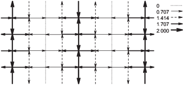
For simplicity, we focus on period-2 CDW, which breaks symmetry and necessarily couples to disorder. On symmetry grounds, the effective Hamiltonian is modeled by a random field Ising model (RFIM), [21]
| (1) |
where is the coupling between the Ising spins, and is a set of uncorrelated, uniformly distributed (rectangular distribution) random variables with zero mean and variance . The notation denotes nearest neighbors. The model is controlled by a single dimensionless parameter, .
The disorder in a RFIM drives fluctuations on many length scales, and consequently many time scales, producing glassy dynamics and a frequency-dependent susceptibility [22]. This result is recapitulated here for the case and extended to the essential case. Analogous to the thermally driven fluctuation of an Ising system at finite temperature, the RFIM has disorder driven fluctuations at zero temperature. A distribution of domain walls of length arises from the domains in the ground state of the RFIM [22].
The appearance of domain walls in RFIM is identified numerically by converting the RFIM to a network flow model [23], and solving the “minimum-cut” problem, for which there are efficient algorithms [24]. Briefly, by careful choice of the parameters of the flow-network and the addition of two fictional source and sink nodes, each cut is made to correspond to a spin configuration such that the minimal cut corresponds to the RFIM ground state configuration. The probability that a domain wall of linear dimension exists in the ground state, , is determined by averaging over many disorder realizations. To help understand the meaning of this quantity, notice that, in the case, a domain wall is just a spin flip. In the disorder-free case, creating a single spin flip costs energy , an energy that, by Jordan-Wigner transformation, can be thought of as a fermion gap. The spin flip can move throughout the system at no energy cost.
In higher dimensions, the analogy is less precise, but the presence of a domain wall results in the collapse of the gap in the Ising system. Most importantly, the size of the domains is controlled by locations of these domain walls. In particular, is the cumulative distribution function of the ordered domains or “clusters” of linear dimension , and therefore
| (2) |
is found to lie on a universal curve [22] which is an asymmetric sigmoid,
| (3) |
where and is numerically fit, and sets a scale for the strength of the disorder. In , is set to as in Ref. 22, in agreement with the analytical result for the special case [25]. In , is numerically fit. The sigmoid’s best fit parameters and control its center and width, respectively, while controls the asymmetry. Physically, determines the onset of the occurrence of domain walls, and how quickly the regime is dominated by the existence of at least one domain wall. The numerical results are summarized in Fig. 2 and Table 1.

The distribution is important because it controls the (necessarily local) susceptibility [26, 22]
| (4) |
This phenomenological argument for the susceptibility captures the essential glassy characteristics resulting from . In principle, the attempt frequency , the fractal dimension , and the length scale are microscopic parameters, which are left undetermined. Notice that the fractal dimension , where is the ambient spatial dimension. For and , the integral simplifies in the small limit to
| (5) |
We have put for clarity and compactness; is strictly increasing for , and vanishes as . The exponent
| (6) |
depends only on the fractal dimension of the domains and on their distribution of sizes via the parameter . Moreover, in both and , the numerical value of was found to lead to (see Table 1).
We now focus on the interaction of the itinerant electrons with the emergent glassy CDW order, assumed to enter as a heat bath of fluctuations of the RFIM. The self energy of the electrons is calculated to leading order in perturbation theory (see FIG. 3), assuming some coupling of the RFIM fluctuations to the electrons, from the form of in Eq. 5 in a reduced graph expansion [27]. It is unnecessary to use the matrix formalism corresponding to the charge order, because, as we shall see, there are no quasiparticles, and hence no possible Fermi surface reconstruction. In terms of the energy of quasiparticles ,
| (7) |
The Fermi and Bose functions and restrict the integration to in the zero-temperature limit we are considering, making the integral vanish for . Because the susceptibility is local the self energy is also local, and the sum over reduces to the density of states at the Fermi surface, :
where , and . From the Kramers-Kronig relations:
| (8) |
where we have introduced a cutoff . Because is slowly varying, we approximate it as a constant with :
| (9) |
where we have taken the largest possible value of the cutoff, , and discarded the subdominant terms in the limit . Because , as , both the real and the imaginary part of the self energy vanish.


The spectral function is plotted in FIG. 4 for several values of . The emergent behavior is of an unusual non-Fermi liquid; for and in the limit,
| (10) |
Provided that or equivalently 11 1 Although we have no lower bound on , the condition is rather mild and in and , respectively., the spectral function vanishes as . The falloff is extremely slow, behaving as a fractional power of a logarithm. Furthermore, and despite the slow falloff, the quasiparticle weight always vanishes, and equivalently the effective mass diverges, as :
| (11) |
Cuprates are reasonably modeled as weakly coupled stacks of layers [29]. The above work addresses isotropic coupling; we now argue that anisotropy will not materially affect the results. Consider the Hamiltonian
| (12) |
where is the in-plane coupling and the interplane coupling. denotes nearest neighbors in the direction, and the neighbors in the plane. The random fields are as before.
Unlike , in there is a order-disorder phase transition. In the isotropic case, i.e., , the zero temperature phase transition occurs at a finite , found numerically to be , in good agreement with previous results [30].
The anisotropic case (with ) is illustrated in Fig. 5. Numerically, a particular value of is fixed, and is varied to identify the phase boundary in the - plane. A simple mean field theory result is also illustrated: as shown earlier [22], in the correlation length
| (13) |
with . Treating the system as a stack of coupled planes, a mean field theory argument suggests the crossover from purely (at weak enough ) to occurs for
| (14) |

The qualitative features are readily understood. When the system decouples as a RFIM, which cannot order (a scenario irrelevant to the cuprates). On the other hand, when the case simplifies to the RFIM, which while it also cannot order, has an exponentially large crossover scale. It is in the latter regime that the fully and stacked results overlap. For weak , the system is disordered and the total energetic contribution from the coupling can be made small relative to the in-plane terms. An interpolation between the and cases is expected in the anisotropic case, which should always result in the supression of a quasiparticle peak.
In conclusion, random field disorder is significant even in the apparently well ordered materials of high temperature superconductors, but its effect is quite different for the two orders, CDW and DDW. Because the symmetry is broken for period-2 CDW, it is susceptible to random field disorder, destroying the Fermi surface, as we have found here by treating it as a RFIM. The disorder results in the glassy susceptibility of Eq. 5, producing a quite unusual non-Fermi liquid. Physically, the glassy dynamics are due to the wide range of scales over which domain walls exist in the ground states of the and RFIM and are characterized by the parameter , which controls susceptibility and in turn the non-Fermi liquid behavior. No Fermi-surface reconstruction can in principle occur, precluding quantum oscillations, up to some important caveats: the coupling parameter must not be too small, and the CDW correlation length cannot be too large relative to the cyclotron radius (see Ref. 31). Truly incommensurate order in the presence of disorder is far too complex and was not addressed in the present work, but can only make things worse as far as quantum oscillations are concerned.
In contrast, DDW modulates bond currents—a Hartree-Fock calculation of DDW is given by Laughlin [32]—which cannot directly couple to potential disorder, even though the order breaks translational symmetry. No non-Fermi liquid behavior is expected. Higher periodicity DDW (for example, period-8) can induce parasitic charge order that can couple to disorder. Being a higher order effect in Landau theory, this coupling may be weak. However, the observed weak CDW involves such a small motion of the atoms, it is hard to believe that it could be the cause of a large magnitude pseudogap. In any case, the short range nature of the CDW combined with RFIM disorder cannot explain quantum oscillations, at least if the resulting electronic state is a non-Fermi liquid. As a third option, if we neglect disorder and assume very long-ranged CDW, (perhaps infinitely long-ranged), Fermi surface reconstruction and quantum oscillation have been shown to be possible [33, 34, 35, 36]. The current experiments, however, do not appear to support such assumptions.
This work was supported by a grant from the National Science Foundation, DMR-1004520. We thank E. Abrahams for discussion. We thank B. J. Ramshaw, S. E. Sebastian and D. Schwab for comments on an earlier version of the manuscript. We also thank C. M. Varma for drawing our attention to Ref. 18.
References
- [1] T. Wu, H. Mayaffre, S. Krämer, M. Horvatić, C. Berthier, W. N. Hardy, R. Liang, D. A. Bonn, and M.-H. Julien, Nature 477, 191 (2011).
- [2] D. LeBoeuf, S. Krämer, W. N. Hardy, R. Liang, D. A. Bonn, and C. Proust, Nature Physics 9, 79 (2012).
- [3] G. Ghiringhelli, M. Le Tacon, M. Minola, S. Blanco-Canosa, C. Mazzoli, N. B. Brookes, G. M. D. Luca, A. Frano, D. G. Hawthorn, F. He, T. Loew, M. M. Sala, D. C. Peets, M. Salluzzo, E. Schierle, R. Sutarto, G. A. Sawatzky, E. Weschke, B. Keimer, and L. Braicovich, Science 337, 821 (2012).
- [4] J. Chang, E. Blackburn, A. T. Holmes, N. B. Christensen, J. Larsen, J. Mesot, R. Liang, D. A. Bonn, W. N. Hardy, A. Watenphul, M. v. Zimmermann, E. M. Forgan, and S. M. Hayden, Nature Physics 8, 871 (2012).
- [5] J. E. Hoffman, Science 295, 466 (2002).
- [6] Y. Kohsaka, C. Taylor, K. Fujita, A. Schmidt, C. Lupien, T. Hanaguri, M. Azuma, M. Takano, H. Eisaki, H. Takagi, S. Uchida, and J. C. Davis, Science 315, 1380 (2007).
- [7] A. J. Achkar, R. Sutarto, X. Mao, F. He, A. Frano, S. Blanco-Canosa, M. L. Tacon, G. Ghiringhelli, L. Braicovich, M. Minola, M. M. Sala, C. Mazzoli, R. Liang, D. A. Bonn, W. N. Hardy, B. Keimer, G. A. Sawatzky, and D. G. Hawthorn, Phys. Rev. Lett. 109, 167001 (2012).
- [8] W. Tabis, Y. Li, M. L. Tacon, L. Braicovich, A. Kreyssig, M. Minola, G. Dellea, E. Weschke, M. J. Veit, M. Ramazanoglu, A. I. Goldman, T. Schmitt, G. Ghiringhelli, N. Barišić, M. K. Chan, C. J. Dorow, G. Yu, X. Zhao, B. Keimer, and M. Greven, Nature Communications 5, 5875 (2014).
- [9] N. Doiron-Leyraud, C. Proust, D. LeBoeuf, J. Levallois, J.-B. Bonnemaison, R. Liang, D. A. Bonn, W. N. Hardy, and L. Taillefer, Nature 447, 565 (2007).
- [10] D. LeBoeuf, N. Doiron-Leyraud, J. Levallois, R. Daou, J.-B. Bonnemaison, N. E. Hussey, L. Balicas, B. J. Ramshaw, R. Liang, D. A. Bonn, W. N. Hardy, S. Adachi, C. Proust, and L. Taillefer, Nature 450, 533 (2007).
- [11] C. Jaudet, D. Vignolles, A. Audouard, J. Levallois, D. LeBoeuf, N. Doiron-Leyraud, B. Vignolle, M. Nardone, A. Zitouni, R. Liang, D. A. Bonn, W. N. Hardy, L. Taillefer, and C. Proust, Phys. Rev. Lett. 100, 187005 (2008).
- [12] S. Chakravarty, Science 319, 735 (2008).
- [13] Y. Zhang, A. V. Maharaj, and S. Kivelson, Phys. Rev. B 91, 085105 (2015).
- [14] S. Chakravarty and H.-Y. Kee, Proc. Natl. Acad. Sci. USA 105, 8835 (2008).
- [15] H. A. Mook, P. Dai, S. M. Hayden, A. Hiess, J. W. Lynn, S. H. Lee, and F. Doǧan, Phys. Rev. B 66, 144513 (2002).
- [16] H. A. Mook, P. Dai, S. M. Hayden, A. Hiess, S. H. Lee, and F. Doǧan, Phys. Rev. B 69, 134509 (2004).
- [17] S. Strässle, B. Graneli, M. Mali, J. Roos, and H. Keller, Phys. Rev. Lett. 106, 097003 (2011).
- [18] C. Hou, D. E. MacLaughlin, and C. M. Varma, Phys. Rev. B 89, 235108 (2014).
- [19] J. Eun, Z. Wang, and S. Chakravarty, Proceedings of the National Academy of Sciences 109, 13198 (2012).
- [20] I. Dimov, P. Goswami, X. Jia, and S. Chakravarty, Phys. Rev. B 78, 134529 (2008).
- [21] A. P. Young, ed., Spin Glasses and Random Fields (World Scientific, Singapore, 1998).
- [22] D. Schwab and S. Chakravarty, Phys. Rev. B 79, 125102 (2009).
- [23] A. K. Hartmann and H. Rieger, Optimization Algorithms in Physics (Wiley-VCH, 2002).
- [24] L. R. Ford and D. R. Fulkerson, Canad. J. Math. 8, 399 (1956).
- [25] K. Binder, Zeitschrift für Physik B Condensed Matter 50, 343 (1983).
- [26] S. Sachdev, Quantum Phase Transitions (Cambridge University Press, 2011).
- [27] E. Abrahams, J. Schmalian, and P. Wölfle, Phys. Rev. B 90, 045105 (2014).
- [28] Although we have no lower bound on , the condition is rather mild and in and , respectively.
- [29] L. Nie, G. Tarjus, and S. A. Kivelson, Proceedings of the National Academy of Sciences 111, 7980 (2014).
- [30] A. A. Middleton and D. S. Fisher, Phys. Rev. B 65, 134411 (2002).
- [31] B. S. Tan, N. Harrison, Z. Zhu, F. Balakirev, B. J. Ramshaw, A. Srivastava, S. A. Sabok, B. Dabrowski, G. G. Lonzarich, and S. E. Sebastian, Proceedings of the National Academy of Sciences , 201504164 (2015).
- [32] R. B. Laughlin, Phys. Rev. B 89, 035134 (2014).
- [33] A. V. Maharaj, P. Hosur, and S. Raghu, Phys. Rev. B 90, 125108 (2014).
- [34] S. E. Sebastian, N. Harrison, F. F. Balakirev, M. M. Altarawneh, P. A. Goddard, R. Liang, D. A. Bonn, W. N. Hardy, and G. G. Lonzarich, Nature 511, 51 (2014).
- [35] A. Allais, D. Chowdhury, and S. Sachdev, Nat Commun 5, 5771 (2014).
- [36] N. Doiron-Leyraud, S. Badoux, S. R. de Cotret, S. Lepault, D. LeBoeuf, F. Laliberté, E. Hassinger, B. J. Ramshaw, D. A. Bonn, W. N. Hardy, R. Liang, J.-H. Park, D. Vignolles, B. Vignolle, L. Taillefer, and C. Proust, Nature Communications 6, 6034 (2015).