The recent discovery of a Higgs particle at the LHC [1] has confirmed the validity of the Standard Model (SM). ATLAS and CMS have found that the Higgs boson has a mass of 125 GeV [2] and that its couplings to gauge bosons and third-generation fermions are consistent with the SM predictions [3, 4]. The experimental uncertainties on Higgs couplings are still sizeable, but they will be progressively reduced, first at the LHC and then at future colliders. Several models of physics beyond the SM will be tested as well, since they generically predict both deviations in those couplings and new particles to be discovered. Supersymmetric (SUSY) extensions of the SM are well known examples of such theories. In a wide class of SUSY models, including the MSSM and the NMSSM, the Higgs sector contains two doublets and possibly singlets [5, 6, 7]. A linear combination of the doublets ($H=\sin\beta\,H_{u}-\cos\beta\,i\sigma_{2}H_{d}^{*}$) behaves as the SM doublet in the decoupling limit of the other Higgs states. We will focus on this regime for definiteness. Our aim is to investigate some properties of such SM-like Higgs field in a particular region of the SUSY parameter space, characterized by large values of certain flavour violating trilinear couplings.

Let us parametrize the neutral component of $H$ as $H^{0}=v+\frac{1}{\sqrt{2}}(h+iG)$, where $v\simeq 174\,{\rm GeV}$ triggers $SU(2)\times U(1)$ breaking, $h$ is the physical Higgs boson and $G$ is the neutral would-be Goldstone boson. Stop squarks are the SUSY particles that couple more strongly to $H^{0}$. Indeed, $F$-terms generate large quartic couplings of the form $y_{t}^{2}|H^{0}|^{2}(|\tilde{t}_{L}|^{2}+|\tilde{t}_{R}|^{2})$, where $y_{t}$ is the SM top Yukawa coupling (i.e., $y_{t}$ is related to the top mass through $m_{t}=y_{t}\,v$ at the tree level). $F$-terms and SUSY-breaking $A$-terms also generate Higgs-stop-stop trilinear couplings. We assume that sizeable Higgs-stop-scharm $A$-terms are present as well, although we do not specify their origin. Hence the trilinear scalar interactions that are relevant to us are

$$V_{(3)}=y_{t}\,H^{0}\,(X_{t}\,\tilde{t}_{R}^{\,*}\,\tilde{t}_{L}+A_{tc}\,\tilde{t}_{R}^{\,*}\,\tilde{c}_{L}+A_{ct}\,\tilde{c}_{R}^{\,*}\,\tilde{t}_{L})+{\rm h.c.}\;,$$

(1)

where we have used the standard notation $X_{t}\equiv A_{t}-\mu^{*}\cot\beta$ and factored out $y_{t}$ for convenience. We complete our parametrization by writing stop and scharm (SUSY-breaking) mass terms as $\tilde{m}^{2}_{t_{L}}|\tilde{t}_{L}|^{2}+\tilde{m}^{2}_{t_{R}}|\tilde{t}_{R}|^{2}+\tilde{m}^{2}_{c_{L}}|\tilde{c}_{L}|^{2}+\tilde{m}^{2}_{c_{R}}|\tilde{c}_{R}|^{2}$. Gauge invariance implies mass terms $\tilde{m}^{2}_{t_{L}}|\tilde{b}_{L}|^{2}+\tilde{m}^{2}_{c_{L}}|\tilde{s}_{L}|^{2}$ for $\tilde{b}_{L}$ and $\tilde{s}_{L}$, the $SU(2)$ partners of $\tilde{t}_{L}$ and $\tilde{c}_{L}$. In general one also expects flavour violating mass terms of $LL$ and $RR$ type, as well as other $LR$ trilinears. The effective low-energy values of all such parameters depend, as usual, both on boundary conditions at some higher scale and on renormalization effects, which include those generated by $A_{tc}$ and $A_{ct}$ themselves. Although we are aware of the latter connection, we decide to explore the region of the phenomenological SUSY parameter space where all flavour violating masses are small, apart from those in eq. (1). In other words, we do not specify either a flavour model or a mechanism of SUSY breaking, treat $A_{tc}$ and $A_{ct}$ as phenomenological parameters (on the same footing as $X_{t}$) and allow them to be as large as the flavour conserving stop and scharm masses. Even in the latter limit the constraints from flavour changing observables are weak or absent, especially for ${\cal O}({\rm TeV})$ squark masses. We will return to this point in a separate paper [8], whereas here we will study the impact of $A_{tc}$ and $A_{ct}$ on a set of flavour conserving quantities, namely:

i)

the mass of the Higgs boson $h$ (Section 2);

ii)

the $\rho$ parameter (Section 3);

iii)

the effective coupling of $h$ to gluons or photons (Section 4);

iv)

the effective coupling of $h$ to charm quarks (Section 5).

In each case we will compute the leading effects and present simple analytical expressions which exhibit the relevant parametric dependences. By ‘leading’ we mean that squarks are integrated out at the one-loop level, at leading order in $y_{t}$ and at lowest order in $v^{2}/\tilde{m}^{2}$, where $\tilde{m}^{2}$ generically denotes a squark mass. In the effective theory language, the latter point means that we evaluate the squark contribution to the operators of lowest dimension ($d$) associated with each of the above quantities, namely:

i)

$|H^{0}|^{4}$ ($d=4$);

ii)

$|H^{\dagger}D_{\mu}H|^{2}$ ($d=6$);

iii)

$|H^{0}|^{2}G_{\mu\nu}G^{\mu\nu}\,,\,|H^{0}|^{2}F_{\mu\nu}F^{\mu\nu}$ ($d=6$);

iv)

$|H^{0}|^{2}H^{0}\,\overline{c_{R}}\,c_{L}+{\rm h.c.}$ ($d=6$).

These different dimensionalities imply different decoupling properties, of course. Squark contributions to $\rho$ and to the effective Higgs couplings are suppressed by a factor $v^{2}/\tilde{m}^{2}$ ($d=6$ operators). On the other hand, corrections to the Higgs mass do not feel that suppression since they are associated to a quartic coupling ($d=4$ operator). In any case, once the appropriate power of $v^{2}/\tilde{m}^{2}$ is taken into account, for each of the above quantities the remaining dependence on mass parameters will be encoded in some dimensionless function. In particular, the dependence on trilinear parameters will appear through powers of $X_{t}/\tilde{m},A_{tc}/\tilde{m},A_{ct}/\tilde{m}$.

In the SM the Higgs mass is $m_{h}^{2}=\lambda v^{2}$ at the tree level, where $\lambda$ is a free parameter that controls the quartic term of the Higgs potential ($V\supset\frac{1}{4}\lambda|H^{0}|^{4}$). The measured value of $m_{h}\simeq 125$ GeV implies $\lambda\simeq 0.5$ at the weak scale. In SUSY scenarios with a SM-like Higgs, $\lambda$ is an effective coupling that can receive contributions from different sources: $\lambda\simeq\sum_{i}\delta\lambda_{i}$. At the tree level the standard $D$-term contribution $\delta\lambda_{D}=\frac{1}{2}(g^{2}+g^{\prime 2})\cos^{2}2\beta$ predicts $m_{h}=m_{Z}|\cos 2\beta|\leq m_{Z}$, significantly lower than 125 GeV. Additional tree-level contributions to $\lambda$ can arise, e.g., from $F$-terms in extensions with singlets [7] or from higher dimension effective operators [9]. Important contributions to $\lambda$ also arise radiatively. The leading ones are generated by top and stop one-loop diagrams [10] and are proportional to $y_{t}^{4}$:

$$\delta\lambda_{\rm log}\simeq\frac{3y_{t}^{4}}{4\pi^{2}}\log\frac{\tilde{m}^{2}_{t}}{m_{t}^{2}}\;\;\;,\;\;\;\delta\lambda_{\rm thr}\simeq\frac{3y_{t}^{4}}{4\pi^{2}}\,\Delta\,.$$

(2)

The first term $\delta\lambda_{\rm log}$ can be interpreted either as the combination of logarithmically divergent top and stop contributions, or as the result of the top-loop-induced running of $\lambda$ from the stop mass scale $\tilde{m}^{2}_{t}\simeq(\tilde{m}^{2}_{t_{L}}\tilde{m}^{2}_{t_{R}})^{1/2}$ to the weak scale ($4\pi^{2}d\lambda/d\log q^{2}=-3y_{t}^{4}+\ldots$). The second term $\delta\lambda_{\rm thr}$ is a finite threshold correction at the stop scale and we parametrize it through $\Delta$, a dimensionless function of squark mass parameters¹¹ 1 More precisely, the tree-level contributions and $\delta\lambda_{\rm thr}$ determine the SM coupling $\lambda$ at the SUSY matching scale. The latter coupling is then renormalized down to the weak scale where $m_{h}$ is evaluated. For recent investigations on the SUSY threshold effect, RG evolution and higher order corrections, see [11] and refs. therein. If one uses the approximate expressions in eq. (2), the factors $y_{t}^{4}$ may be evaluated at the scales suggested in [12], i.e. at $(m_{t}\tilde{m}_{t})^{1/2}$ in $\delta\lambda_{\rm log}$ and at $\tilde{m}_{t}$ in $\delta\lambda_{\rm thr}$.. In the flavour conserving limit, $\Delta$ contains quadratic and quartic powers of $X_{t}$. As well known, an appropriate choice of $X_{t}$ can give a substantial contribution to $\Delta$, which translates into a correction $\delta m_{h}^{2}\simeq\delta\lambda_{\rm thr}v^{2}$ to the Higgs mass. In the often quoted limit $\tilde{m}^{2}_{t_{L}}=\tilde{m}^{2}_{t_{R}}=\tilde{m}^{2}_{t}$, for instance, $\Delta=|X_{t}|^{2}/\tilde{m}^{2}_{t}-\frac{1}{12}|X_{t}|^{4}/\tilde{m}^{4}_{t}$ reaches its maximal value $\Delta_{\rm max}=3$ at $|X_{t}|=\sqrt{6}\,\tilde{m}_{t}$. The corresponding linear correction to $m_{h}$ is about $15$–$20$ GeV. We recall that, as often emphasized, a large threshold correction is welcome because it allows a smaller stop mass scale in the logarithmic term (e.g., $\tilde{m}_{t}$ around 1 TeV rather than in the multi-TeV range). However, the knowledge of the threshold correction is important also in more general scenarios.

Our purpose in this Section is to generalize the one-loop calculation of $\Delta$ by including the effect of the flavour violating $A$-terms $A_{tc}$ and $A_{ct}$ of eq. (1), which couple the Higgs field to stop and scharm squarks. The one-loop stop/scharm diagrams that contribute to $\Delta$ at ${\cal O}(y_{t}^{4})$ are shown in Fig. 1.

Those in the first (second) row are quadratic (quartic) in $X_{t},A_{tc},A_{ct}$ and give positive (negative) contributions to $\Delta$. We find:

	$\displaystyle\Delta$	$\displaystyle=$	$\displaystyle\frac{|X_{t}|^{2}}{\tilde{m}^{2}_{t_{L}}-\tilde{m}^{2}_{t_{R}}}\log\frac{\tilde{m}^{2}_{t_{L}}}{\tilde{m}^{2}_{t_{R}}}+\frac{|A_{ct}|^{2}}{\tilde{m}^{2}_{c_{R}}}f_{1}\!\left(\frac{\tilde{m}^{2}_{t_{L}}}{\tilde{m}^{2}_{c_{R}}}\right)+\frac{|A_{tc}|^{2}}{\tilde{m}^{2}_{c_{L}}}f_{1}\!\left(\frac{\tilde{m}^{2}_{t_{R}}}{\tilde{m}^{2}_{c_{L}}}\right)$		(3)
			$\displaystyle-\frac{1}{2}\left[\frac{|X_{t}|^{4}}{\tilde{m}^{4}_{t_{L}}}f_{2}\!\left(\frac{\tilde{m}^{2}_{t_{R}}}{\tilde{m}^{2}_{t_{L}}}\right)+\frac{|A_{ct}|^{4}}{\tilde{m}^{4}_{c_{R}}}f_{2}\!\left(\frac{\tilde{m}^{2}_{t_{L}}}{\tilde{m}^{2}_{c_{R}}}\right)+\frac{|A_{tc}|^{4}}{\tilde{m}^{4}_{c_{L}}}f_{2}\!\left(\frac{\tilde{m}^{2}_{t_{R}}}{\tilde{m}^{2}_{c_{L}}}\right)\right]$
			$\displaystyle-\frac{|X_{t}|^{2}|A_{ct}|^{2}}{\tilde{m}^{2}_{c_{R}}-\tilde{m}^{2}_{t_{R}}}\left[\frac{1}{\tilde{m}^{2}_{t_{R}}}f_{1}\left(\frac{\tilde{m}^{2}_{t_{L}}}{\tilde{m}^{2}_{t_{R}}}\right)-\frac{1}{\tilde{m}^{2}_{c_{R}}}f_{1}\left(\frac{\tilde{m}^{2}_{t_{L}}}{\tilde{m}^{2}_{c_{R}}}\right)\right]$
			$\displaystyle-\frac{|X_{t}|^{2}|A_{tc}|^{2}}{\tilde{m}^{2}_{c_{L}}-\tilde{m}^{2}_{t_{L}}}\left[\frac{1}{\tilde{m}^{2}_{t_{L}}}f_{1}\left(\frac{\tilde{m}^{2}_{t_{R}}}{\tilde{m}^{2}_{t_{L}}}\right)-\frac{1}{\tilde{m}^{2}_{c_{L}}}f_{1}\left(\frac{\tilde{m}^{2}_{t_{R}}}{\tilde{m}^{2}_{c_{L}}}\right)\right]\,,$

where $f_{i}(x)$ are positive functions [with $f_{1}(1)=\frac{1}{2}$, $f_{2}(1)=\frac{1}{6}$]:

$$f_{1}(x)=-\frac{1}{(x-1)^{2}}\log x+\frac{1}{x-1}\;\;\;,\;\;\;f_{2}(x)=\frac{x+1}{(x-1)^{3}}\log x-\frac{2}{(x-1)^{2}}\,.$$

(4)

The overall size of the threshold function $\Delta$ as well as its sign depend on the competition of positive and negative terms, in analogy to the familiar case with $X_{t}$ only. The novel contributions induced by $A_{ct}$ and $A_{tc}$ can be of the same order as the standard ones driven by $X_{t}$. As the total effect depends on several mass parameters, a pre-fixed value of $\Delta$ is associated with some hypersurface in a multi-dimensional parameter space. To simplify the discussion, suppose that $(\tilde{t}_{L},\tilde{t}_{R})$ have a common mass $\tilde{m}^{2}_{t}$ ($\simeq\tilde{m}^{2}_{t_{L}}\simeq\tilde{m}^{2}_{t_{R}}$) and that $(\tilde{c}_{L},\tilde{c}_{R})$ have a common mass $\tilde{m}^{2}_{c}$ ($\simeq\tilde{m}^{2}_{c_{L}}\simeq\tilde{m}^{2}_{c_{R}}$). In this limit, the threshold function becomes:

	$\displaystyle\Delta$	$\displaystyle=$	$\displaystyle\frac{|X_{t}|^{2}}{\tilde{m}^{2}_{t}}+\frac{|A_{ct}|^{2}+|A_{tc}|^{2}}{\tilde{m}^{2}_{c}}f_{1}\left(\frac{\tilde{m}^{2}_{t}}{\tilde{m}^{2}_{c}}\right)$		(5)
		$\displaystyle-$	$\displaystyle\left[\frac{1}{12}\frac{|X_{t}|^{4}}{\tilde{m}^{4}_{t}}+\frac{1}{2}\frac{|A_{ct}|^{4}+|A_{tc}|^{4}}{\tilde{m}^{4}_{c}}f_{2}\left(\frac{\tilde{m}^{2}_{t}}{\tilde{m}^{2}_{c}}\right)+\frac{|X_{t}|^{2}}{\tilde{m}^{2}_{t}}\cdot\frac{|A_{ct}|^{2}+|A_{tc}|^{2}}{\tilde{m}^{2}_{c}}f_{3}\left(\frac{\tilde{m}^{2}_{t}}{\tilde{m}^{2}_{c}}\right)\right]\;,$

where $f_{3}(x)$ is another positive function [with $f_{3}(1)=\frac{1}{6}$]:

$$f_{3}(x)=-\frac{x}{(x-1)^{3}}\log x+\frac{x+1}{2(x-1)^{2}}\,.$$

(6)

A further simplification occurs in the fully degenerate limit $\tilde{m}^{2}_{c}=\tilde{m}^{2}_{t}=\tilde{m}^{2}$:

$$\Delta=\frac{|X_{t}|^{2}}{\tilde{m}^{2}}+\frac{|A_{tc}|^{2}+|A_{ct}|^{2}}{2\,\tilde{m}^{2}}-\frac{|X_{t}|^{4}+|A_{tc}|^{4}+|A_{ct}|^{4}+2|X_{t}|^{2}(|A_{tc}|^{2}+|A_{ct}|^{2})}{12\,\tilde{m}^{4}}\;.$$

(7)

Let us consider, for instance, the simplified expression in eq. (7). Here $\Delta$ is a function of only three dimensionless variables, namely $(x_{t},a_{tc},a_{ct})\equiv(|X_{t}|/\tilde{m},|A_{tc}|/\tilde{m},|A_{ct}|/\tilde{m})$. By a simple analytical study, we find the interesting result that $\Delta$ is maximal at the ‘standard point’ $(x_{t},a_{tc},a_{ct})=(\sqrt{6},0,0)$, where $\Delta=3$. There are other extremal points where the flavour changing trilinears do not vanish, namely $(0,\sqrt{3},0)$, $(0,0,\sqrt{3})$ and $(0,\sqrt{3},\sqrt{3})$. At such extrema, which are saddle points, $\Delta$ take values $3/4$, $3/4$ and $3/2$, respectively. In a significant portion of the three-dimensional parameter space spanned by $(x_{t},a_{tc},a_{ct})$ one can obtain $\Delta\stackrel{{\scriptstyle>}}{{{}_{\sim}}}1$. The role of $x_{t}$ is crucial in order to reach $\Delta\stackrel{{\scriptstyle>}}{{{}_{\sim}}}2$.

Consider now a slightly more general scenario in which stop and scharm masses are characterized by two distinct parameters $\tilde{m}^{2}_{t}$ and $\tilde{m}^{2}_{c}$, such that $\Delta$ is given by eq. (5). The parameter space can be described by three coordinates associated with the trilinear couplings, which we take as $(x_{t},a_{tc},a_{ct})\equiv(|X_{t}|/\tilde{m}_{t},|A_{tc}|/\tilde{m}_{c},|A_{ct}|/\tilde{m}_{c})$, plus the ratio $r\equiv\tilde{m}_{c}/\tilde{m}_{t}$, which we treat as an external parameter. By an analytical study of $\Delta$ for fixed $r$, we find the standard extremum at $(\sqrt{6},0,0)$ as well as other ones at $(0,a_{*},0)$, $(0,0,a_{*})$ and $(0,a_{*},a_{*})$, where $a_{*}=\sqrt{f_{1}/f_{2}}$ and $f_{i}\equiv f_{i}(1/r^{2})$. Another extremum (a saddle point) appears for $1<r\stackrel{{\scriptstyle<}}{{{}_{\sim}}}5$. The extremum at $(0,a_{*},a_{*})$ is interesting because it is a local maximum for $r>1$. The associated value of $\Delta$ is $\Delta_{*}=f_{1}^{2}/f_{2}$, which increases for increasing $r$: for $r=(0.5;\,1;\,2;\,3;\,4;\,5;\,6)$ one finds $\Delta_{*}\simeq(0.9;\,1.5;\,2.3;\,2.9;\,3.4;\,3.7;\,4)$. This behaviour follows from the mild (logarithmic) enhancement of the coefficient functions $f_{1}$ and $f_{2}$, which is easily interpreted through the diagrams in Fig. 1. The other extrema $(0,a_{*},0)$ and $(0,0,a_{*})$ are saddle points and have $\Delta=\frac{1}{2}\Delta_{*}$. By comparing the reported values of $\Delta_{*}$ with $\Delta=3$ at the standard extremum $(\sqrt{6},0,0)$, we can see that the latter point is no longer the absolute maximum for $r\stackrel{{\scriptstyle>}}{{{}_{\sim}}}3$. For $r\stackrel{{\scriptstyle>}}{{{}_{\sim}}}5$, it is not even a local maximum and becomes a saddle point (namely, $\Delta$ increases if ones moves away from that point in the flavour violating directions).

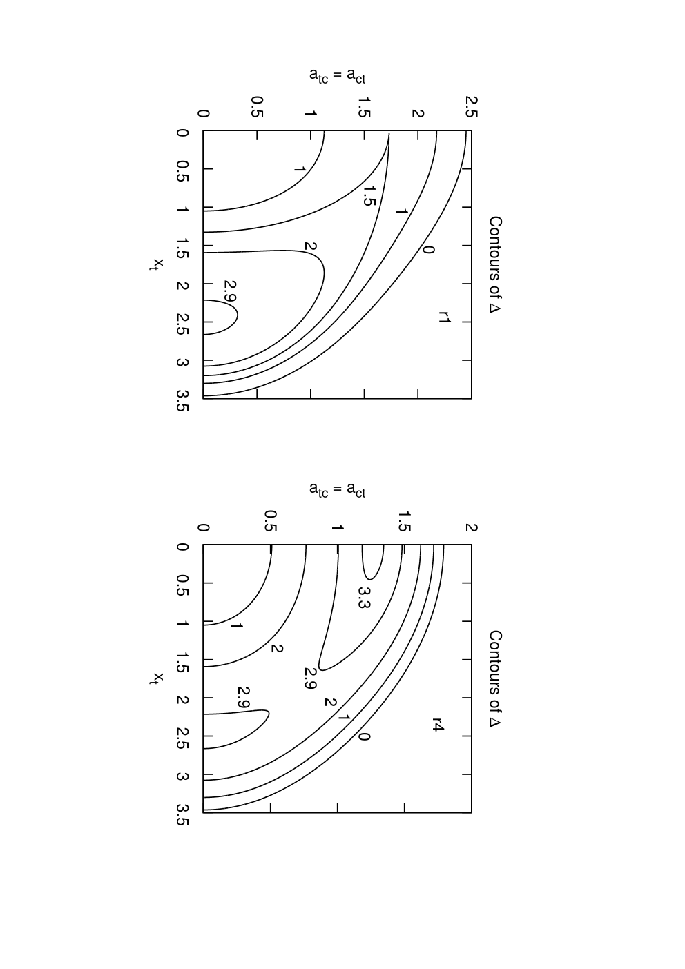
The behaviour of the threshold function $\Delta$ is further illustrated in Fig. 2, where some iso-contours are shown in a two-dimensional subspace spanned by $x_{t}$ and $a_{tc}=a_{ct}$, for either $r=1$ (left panel) or $r=4$ (right panel). The case $r=1$ (namely, $\tilde{m}_{c}=\tilde{m}_{t}$) is the degenerate limit, already discussed above. One can easily recognize the standard maximum at $x_{t}=\sqrt{6}$ (and $a_{tc}=a_{ct}=0$), where $\Delta=3$, and the other extremum (saddle point) at $a_{tc}=a_{ct}=\sqrt{3}$ (and $x_{t}=0$), where $\Delta=1.5$. The case $r=4$ (namely, $\tilde{m}_{c}=4\,\tilde{m}_{t}$) is an example of a moderately hierarchical scenario. The extremum on the $a_{tc}=a_{ct}$ axis has turned into a maximum, and $\Delta$ is higher there than at the standard maximum on the $x_{t}$ axis. More generally, by comparing this case with the previous one, one can notice the expansion of the region of parameter space where $\Delta\stackrel{{\scriptstyle>}}{{{}_{\sim}}}2$, which translates into a linear correction to $m_{h}$ larger than about $10$ GeV. As $\Delta\stackrel{{\scriptstyle>}}{{{}_{\sim}}}3$ can also be obtained in such hierarchical scenarios, even shifts of ${\cal O}(20)$ GeV are possible. In summary, significant positive threshold corrections to the Higgs mass can be achieved in a variety of ways, by suitable combinations of the flavour conserving and flavour violating trilinear couplings. If any of such parameters is too large, though, the corrections quickly become negative, since $\Delta$ is then dominated by negative quartic terms. In our examples in Fig. 2 this occurs to the right of the iso-contours where $\Delta=0$. Such parameter regions are also disfavoured because the tree-level potential can become unbounded from below along coloured directions or develop colour-breaking minima [13, 14].

A side remark may be added about the impact of sizeable values of $A_{tc}$ and/or $A_{ct}$ on the naturalness of the weak scale. In fact, although we have chosen to avoid discussing renormalization effects above the SUSY scale, it should be mentioned that the soft mass of the Higgs doublet $H_{u}$, i.e. $\tilde{m}^{2}_{H_{u}}$, receives logarithmic corrections proportional to $|A_{t}|^{2}+|A_{tc}|^{2}+|A_{ct}|^{2}$. Therefore fine-tuning issues are not alleviated by the presence of $A_{tc}$ and $A_{ct}$, particularly in case such parameters are of order $\tilde{m}_{c}$ and the latter is much larger than $\tilde{m}_{t}$.

We conclude this Section by some comments on earlier results presented in the literature. The influence of flavour violating $A$-terms on $m_{h}$ was noticed in [15] and confirmed in [16]. However, such papers put a special emphasis on the potentially large negative effect of such trilinear couplings on the Higgs mass, which in fact was used to constrain their magnitude. On the other hand, it was recently pointed out in [17] that a sizeable positive effect on $m_{h}$ can also be achieved, especially in the case of a hierarchical squark spectrum ($\tilde{m}^{2}_{c}\gg\tilde{m}^{2}_{t}$, in our notation). Our study confirms this observation. Upon comparing our analytical results with those presented in [17], though, we have found agreement only in the degenerate case [$\tilde{m}^{2}_{c}=\tilde{m}^{2}_{t}$, eq. (7)], not in the non-degenerate one [$\tilde{m}^{2}_{c}\neq\tilde{m}^{2}_{t}$, eq. (5)].

In the previous Section we have examined certain SUSY corrections to the quartic operator $|H^{0}|^{4}$, which controls the mass of the physical Higgs boson $h\subset H^{0}$. Other properties of $h$ will be investigated in subsequent Sections. Here, instead, we will discuss the impact of SUSY corrections to the $\rho$ parameter, where only the expectation value $\langle|H^{0}|\rangle=v$ is relevant. We select $\delta\rho$ ($=\epsilon_{1}=\alpha\,\delta T$) as the most representative quantity that affects electroweak precision observables, and recall that new physics contributions to $\delta\rho$ are constrained to be at the per mille level at most [18]. For instance, $\delta\rho$ corrects the SM predictions for the $W$ mass $m^{2}_{W}$ and the effective leptonic weak mixing angle $\sin^{2}\theta^{\ell}_{\rm eff}$ by an amount $\delta m_{W}^{2}/m_{W}^{2}\simeq-\delta\sin^{2}\theta^{\ell}_{\rm eff}\,/s^{2}_{w}\simeq a\,\delta\rho$, where $s^{2}_{w}\simeq 0.23$ and $a=c_{w}^{2}/(c_{w}^{2}-s_{w}^{2})\simeq 1.4$. In particular, a positive $\delta\rho\simeq 10^{-3}$ would induce $\delta m_{W}\simeq 60\,{\rm MeV}$. This can be taken as a maximal allowed shift, since the current deviation on $m_{W}$ is $m_{W}^{\rm SM}-m_{W}^{\rm exp}\simeq-25\,{\rm MeV}$, with a one-sigma error of about $17\,{\rm MeV}$. More stringent constraints on $\delta\rho$ are expected from future measurements at the LHC and at other proposed colliders. For general new physics, a full analysis should include other possible sources of corrections to $m^{2}_{W}$ and $\sin^{2}\theta^{\ell}_{\rm eff}$, such as the $S$ parameter. In our case, though, these effects are subleading (they are at most ${\cal O}(g^{2}y_{t}^{2})$, therefore smaller than the ${\cal O}(y_{t}^{4})$ effects associated with $\delta\rho$).

Squark contributions to $\delta\rho$ can be evaluated through $\delta\rho=[\Pi_{33}(0)-\Pi_{WW}(0)]/m_{W}^{2}$, where $\Pi_{33}(0)$ and $\Pi_{WW}(0)$ are the self-energies of $W^{3}$ and $W^{\pm}$ at zero momentum (up to the usual factor $g_{\mu\nu}$). Diagrammatic computations have often been performed by diagonalizing the squark mass matrices and keeping the full dependence on $v$ [19, 20, 21]. As already declared, we choose to evaluate diagrams by explicitly inserting Higgs lines and looking for the leading non-vanishing terms in a $v^{2}$ expansion. At ${\cal O}(v^{0})$, both $\Pi_{33}(0)$ and $\Pi_{WW}(0)$ separately vanish by gauge invariance. At ${\cal O}(v^{2})$, those self-energies receive equal contributions, so there is no net $\delta\rho$ at this order. The leading contributions to $\delta\rho$ arise from ${\cal O}(v^{4})$ terms in $W^{a}$ self-energies, so $\delta\rho\sim v^{2}/\tilde{m}^{2}$. In fact, as well known, such corrections are associated with the $d=6$ effective operator $|H^{\dagger}D_{\mu}H|^{2}$: if $c_{\rho}$ is the coefficient of the latter, $\delta\rho\simeq-c_{\rho}v^{2}$. As the relevant $W^{a}$ self-energies require (at least) four Higgs insertions, we find it very convenient to group the one-loop squark diagrams that contribute to them into three classes, as shown schematically in Fig. 3.

The symbols $\tilde{q}_{L}^{\,i},\tilde{q}_{L}^{\prime\,i}$ generically denote up-type or down-type squarks of the $i$-th left-handed doublet, so it is understood that $\tilde{q}_{L}^{\,i}$ and $\tilde{q}_{L}^{\prime\,i}$ are equal (different) if they couple to $W^{3}$ ($W^{\pm}$). It is both useful and not restrictive to consider a basis where the $3\times 3$ mass matrix $\tilde{m}_{Q}^{2}$ of $SU(2)$ doublets is diagonal, so flavour transitions can only occur at Higgs vertices or in $\tilde{q}_{R}$ propagators. Consider the first class of diagrams in Fig. 3. Each bilinear $|\tilde{q}_{L}^{\,i}|^{2}$ has the same quartic coupling to $|W^{\pm}|^{2}$ and to $\frac{1}{2}(W^{3})^{2}$, by $SU(2)$ invariance. This implies that there are equal contributions to $\Pi_{33}(0)$ and $\Pi_{WW}(0)$, so the net contribution to $\delta\rho$ is zero. A similar argument can be applied to the second class of diagrams. Again, the $SU(2)$ properties of the $W^{a}$-$\tilde{q}_{L}^{\,i}$-$\tilde{q}_{L}^{\prime\,i}$ vertices imply equal contributions to $\Pi_{33}(0)$ and $\Pi_{WW}(0)$ from each doublet, hence zero contribution to $\delta\rho$. Thus we conclude that only diagrams in the third class are relevant to $\delta\rho$.

Our previous classification and conclusion are very general and go beyond the specific framework we are interested in. Let us now specialize all that to our case. Since we are looking for leading effects in $y_{t}$, the Higgs insertions in the third class of diagrams in Fig. 3 should involve $\tilde{t}_{L}$ or $\tilde{c}_{L}$, so the external gauge bosons are $W^{3}$-$W^{3}$. The stop/scharm diagrams that contribute to the $\rho$ parameter at ${\cal O}(y_{t}^{4})$ are shown in Fig. 4.

Apart from the first diagram, the other ones are related to most of those in Fig. 1, namely, those where two external $W^{3}$ bosons can be attached to two distinct $\tilde{q}_{L}$ propagators. The first diagram in Fig. 4 gives a positive contribution to $\delta\rho$. The other ones in the first (second) row are quadratic (quartic) in trilinear couplings and give negative (positive) contributions. The result of our computation is:

	$\displaystyle\delta\rho$	$\displaystyle=$	$\displaystyle\frac{3y_{t}^{4}}{16\pi^{2}}\,\frac{v^{2}}{\tilde{m}^{2}_{t_{L}}}\left\{\frac{1}{6}-\frac{|X_{t}|^{2}}{\tilde{m}^{2}_{t_{R}}}g_{1}\!\left(\frac{\tilde{m}^{2}_{t_{L}}}{\tilde{m}^{2}_{t_{R}}}\right)-\frac{|A_{ct}|^{2}}{\tilde{m}^{2}_{c_{R}}}g_{1}\!\left(\frac{\tilde{m}^{2}_{t_{L}}}{\tilde{m}^{2}_{c_{R}}}\right)\right.$		(8)
			$\displaystyle+\frac{|X_{t}|^{4}}{\tilde{m}^{4}_{t_{R}}}g_{2}\!\left(\frac{\tilde{m}^{2}_{t_{L}}}{\tilde{m}^{2}_{t_{R}}}\right)+\frac{|A_{ct}|^{4}}{\tilde{m}^{4}_{c_{R}}}g_{2}\!\left(\frac{\tilde{m}^{2}_{t_{L}}}{\tilde{m}^{2}_{c_{R}}}\right)+\frac{|A_{tc}|^{4}}{\tilde{m}^{4}_{c_{L}}}\cdot\frac{\tilde{m}^{2}_{t_{L}}}{\tilde{m}^{2}_{c_{L}}}g_{2}\!\left(\frac{\tilde{m}^{2}_{t_{R}}}{\tilde{m}^{2}_{c_{L}}}\right)$
			$\displaystyle+\frac{|X_{t}|^{2}|A_{ct}|^{2}}{\tilde{m}^{2}_{c_{R}}-\tilde{m}^{2}_{t_{R}}}\left[\frac{1}{\tilde{m}^{2}_{t_{R}}}g_{1}\!\left(\frac{\tilde{m}^{2}_{t_{L}}}{\tilde{m}^{2}_{t_{R}}}\right)-\frac{1}{\tilde{m}^{2}_{c_{R}}}g_{1}\!\left(\frac{\tilde{m}^{2}_{t_{L}}}{\tilde{m}^{2}_{c_{R}}}\right)\right]$
			$\displaystyle+2\frac{|X_{t}|^{2}|A_{tc}|^{2}}{(\tilde{m}^{2}_{c_{L}}-\tilde{m}^{2}_{t_{L}})^{2}}\left[f_{3}\!\left(\frac{\tilde{m}^{2}_{t_{R}}}{\tilde{m}^{2}_{t_{L}}}\right)+\frac{\tilde{m}^{2}_{t_{L}}}{\tilde{m}^{2}_{c_{L}}}f_{3}\!\left(\frac{\tilde{m}^{2}_{t_{R}}}{\tilde{m}^{2}_{c_{L}}}\right)\right.$
			$\displaystyle\left.\left.+\frac{\tilde{m}^{2}_{t_{L}}}{\tilde{m}^{2}_{c_{L}}-\tilde{m}^{2}_{t_{L}}}\left(f_{1}\!\left(\frac{\tilde{m}^{2}_{t_{R}}}{\tilde{m}^{2}_{t_{L}}}\right)-f_{1}\!\left(\frac{\tilde{m}^{2}_{t_{R}}}{\tilde{m}^{2}_{c_{L}}}\right)\right)\right]\right\}\;,$

where $f_{1}(x)$ and $f_{3}(x)$ have been defined in eqs. (4) and (6), and $g_{i}(x)$ are other positive functions [with $g_{1}(0)=\frac{1}{3}$, $g_{1}(1)=\frac{1}{12}$, $g_{2}(0)=\frac{1}{6}$, $g_{2}(1)=\frac{1}{60}$]:

$$g_{1}(x)=\frac{x}{(x-1)^{4}}\log x+\frac{x^{2}-5x-2}{6(x-1)^{3}}\;\;\;,\;\;\;g_{2}(x)=-\frac{x(x+1)}{(x-1)^{5}}\log x+\frac{x^{2}+10x+1}{6(x-1)^{4}}\;.$$

(9)

The structure of eq. (8) resembles that of $\Delta$ in eq. (3). Flavour conserving and flavour changing trilinears appear on the same footing and can give effects of the same order. At variance with $\Delta$, though, $\delta\rho$ is not left-right symmetric and is suppressed by an overall factor $v^{2}/\tilde{m}^{2}_{t_{L}}$. All such features are expected, of course. In the simplified scenario where $\tilde{m}^{2}_{t_{L}}\simeq\tilde{m}^{2}_{t_{R}}\simeq\tilde{m}^{2}_{t}$ and $\tilde{m}^{2}_{c_{L}}\simeq\tilde{m}^{2}_{c_{R}}\simeq\tilde{m}^{2}_{c}$, the above result reads:

	$\displaystyle\delta\rho$	$\displaystyle=$	$\displaystyle\frac{3y_{t}^{4}}{16\pi^{2}}\,\frac{v^{2}}{\tilde{m}^{2}_{t}}\left\{\frac{1}{6}-\frac{1}{12}\frac{|X_{t}|^{2}}{\tilde{m}^{2}_{t}}-\frac{|A_{ct}|^{2}}{\tilde{m}^{2}_{c}}g_{1}\!\left(\frac{\tilde{m}^{2}_{t}}{\tilde{m}^{2}_{c}}\right)\right.$		(10)
			$\displaystyle+\frac{1}{60}\frac{|X_{t}|^{4}}{\tilde{m}^{4}_{t}}+\left(\frac{|A_{ct}|^{4}}{\tilde{m}^{4}_{c}}+\frac{|A_{tc}|^{4}}{\tilde{m}^{4}_{c}}\cdot\frac{\tilde{m}^{2}_{t}}{\tilde{m}^{2}_{c}}\right)g_{2}\!\left(\frac{\tilde{m}^{2}_{t}}{\tilde{m}^{2}_{c}}\right)$
			$\displaystyle\left.+\frac{|X_{t}|^{2}}{\tilde{m}^{2}_{t}}\left[\frac{|A_{ct}|^{2}}{\tilde{m}^{2}_{c}}g_{3}\!\left(\frac{\tilde{m}^{2}_{t}}{\tilde{m}^{2}_{c}}\right)+2\frac{|A_{tc}|^{2}}{\tilde{m}^{2}_{c}}\cdot\frac{\tilde{m}^{2}_{t}}{\tilde{m}^{2}_{c}}\,g_{2}\!\left(\frac{\tilde{m}^{2}_{t}}{\tilde{m}^{2}_{c}}\right)\right]\right\}\;,$

where $g_{3}(x)$ is another positive function [with $g_{3}(0)=\frac{1}{12}$, $g_{3}(1)=\frac{1}{30}$]:

$$g_{3}(x)=\frac{x^{2}}{(x-1)^{5}}\log x+\frac{x^{3}-7x^{2}-7x+1}{12(x-1)^{4}}\;.$$

(11)

References

- [1] S. Chatrchyan et al. [CMS Collaboration], Phys. Lett. B 716 (2012) 30 [arXiv:1207.7235 [hep-ex]]; G. Aad et al. [ATLAS Collaboration], Phys. Lett. B 716 (2012) 1 [arXiv:1207.7214 [hep-ex]].
- [2] G. Aad et al. [ATLAS and CMS Collaborations], Phys. Rev. Lett. 114 (2015) 191803 [arXiv:1503.07589 [hep-ex]].
- [3] V. Khachatryan et al. [CMS Collaboration], Eur. Phys. J. C 75 (2015) 5, 212 [arXiv:1412.8662 [hep-ex]].
- [4] The ATLAS Collaboration, ATLAS-CONF-2015-007.
- [5] H. P. Nilles, Phys. Rept. 110 (1984) 1; H. E. Haber and G. L. Kane, Phys. Rept. 117 (1985) 75; S. P. Martin, Adv. Ser. Direct. High Energy Phys. 21 (2010) 1 [hep-ph/9709356].
- [6] A. Djouadi, Phys. Rept. 459 (2008) 1 [hep-ph/0503173].
- [7] M. Drees, Int. J. Mod. Phys. A 4 (1989) 3635; J. R. Ellis, J. F. Gunion, H. E. Haber, L. Roszkowski and F. Zwirner, Phys. Rev. D 39 (1989) 844; U. Ellwanger, C. Hugonie and A. M. Teixeira, Phys. Rept. 496, 1 (2010) [arXiv:0910.1785 [hep-ph]].
- [8] A. Brignole and P. Paradisi, in preparation.
- [9] A. Strumia, Phys. Lett. B 466 (1999) 107 [hep-ph/9906266]; N. Polonsky and S. Su, Phys. Lett. B 508 (2001) 103 [arXiv:hep-ph/0010113]; A. Brignole, J. A. Casas, J. R. Espinosa and I. Navarro, Nucl. Phys. B 666 (2003) 105 [arXiv:hep-ph/0301121]; M. Dine, N. Seiberg and S. Thomas, Phys. Rev. D 76 (2007) 095004 [arXiv:0707.0005 [hep-ph]]; I. Antoniadis, E. Dudas, D. M. Ghilencea and P. Tziveloglou, Nucl. Phys. B 808 (2009) 155 [arXiv:0806.3778 [hep-ph]]; Nucl. Phys. B 831 (2010) 133 [arXiv:0910.1100 [hep-ph]].
- [10] Y. Okada, M. Yamaguchi and T. Yanagida, Prog. Theor. Phys. 85 (1991) 1; Phys. Lett. B 262 (1991) 54; J. R. Ellis, G. Ridolfi and F. Zwirner, Phys. Lett. B 257 (1991) 83; Phys. Lett. B 262 (1991) 477; H. E. Haber and R. Hempfling, Phys. Rev. Lett. 66 (1991) 1815; Phys. Rev. D 48 (1993) 4280 [hep-ph/9307201]; R. Barbieri, M. Frigeni and F. Caravaglios, Phys. Lett. B 258 (1991) 167; J. R. Espinosa and M. Quiros, Phys. Lett. B 266 (1991) 389; P. H. Chankowski, S. Pokorski and J. Rosiek, Phys. Lett. B 274 (1992) 191; A. Brignole, Phys. Lett. B 281 (1992) 284.
- [11] E. Bagnaschi, G. F. Giudice, P. Slavich and A. Strumia, JHEP 1409 (2014) 092 [arXiv:1407.4081 [hep-ph]].
- [12] H. E. Haber, R. Hempfling and A. H. Hoang, Z. Phys. C 75 (1997) 539 [hep-ph/9609331].
- [13] J. M. Frere, D. R. T. Jones and S. Raby, Nucl. Phys. B 222 (1983) 11; L. Alvarez-Gaume, J. Polchinski and M. B. Wise, Nucl. Phys. B 221 (1983) 495.
- [14] J. A. Casas and S. Dimopoulos, Phys. Lett. B 387 (1996) 107 [hep-ph/9606237]; J. h. Park, Phys. Rev. D 83 (2011) 055015 [arXiv:1011.4939 [hep-ph]].
- [15] J. Cao, G. Eilam, K. i. Hikasa and J. M. Yang, Phys. Rev. D 74 (2006) 031701 [hep-ph/0604163].
- [16] M. Arana-Catania, S. Heinemeyer, M. J. Herrero and S. Penaranda, JHEP 1205 (2012) 015 [arXiv:1109.6232 [hep-ph]]; Phys. Rev. D 90 (2014) 7, 075003 [arXiv:1405.6960 [hep-ph]].
- [17] K. Kowalska, JHEP 1409 (2014) 139 [arXiv:1406.0710 [hep-ph]].
- [18] M. Baak et al. [Gfitter Group Collaboration], Eur. Phys. J. C 74 (2014) 3046 [arXiv:1407.3792 [hep-ph]].
- [19] R. Barbieri and L. Maiani, Nucl. Phys. B 224 (1983) 32.
- [20] C. S. Lim, T. Inami and N. Sakai, Phys. Rev. D 29 (1984) 1488; M. Drees and K. Hagiwara, Phys. Rev. D 42 (1990) 1709.
- [21] S. Heinemeyer, W. Hollik, F. Merz and S. Penaranda, Eur. Phys. J. C 37 (2004) 481 [hep-ph/0403228]; S. Heinemeyer, W. Hollik and G. Weiglein, Phys. Rept. 425 (2006) 265 [hep-ph/0412214].
- [22] B. Henning, X. Lu and H. Murayama, arXiv:1404.1058 [hep-ph]; arXiv:1412.1837 [hep-ph].
- [23] A. David et al. [LHC Higgs Cross Section Working Group Collaboration], arXiv:1209.0040 [hep-ph].
- [24] J. R. Ellis, M. K. Gaillard and D. V. Nanopoulos, Nucl. Phys. B 106 (1976) 292; M. A. Shifman, A. I. Vainshtein, M. B. Voloshin and V. I. Zakharov, Sov. J. Nucl. Phys. 30 (1979) 711 [Yad. Fiz. 30 (1979) 1368].
- [25] A. Djouadi, Phys. Lett. B 435 (1998) 101 [hep-ph/9806315].
- [26] K. Blum, R. T. D’Agnolo and J. Fan, JHEP 1301 (2013) 057 [arXiv:1206.5303 [hep-ph]]; M. R. Buckley and D. Hooper, Phys. Rev. D 86 (2012) 075008 [arXiv:1207.1445 [hep-ph]]; J. R. Espinosa, C. Grojean, V. Sanz and M. Trott, JHEP 1212 (2012) 077 [arXiv:1207.7355 [hep-ph]]; A. Delgado, G. F. Giudice, G. Isidori, M. Pierini and A. Strumia, Eur. Phys. J. C 73 (2013) 3, 2370 [arXiv:1212.6847 [hep-ph]]; M. Carena, S. Gori, N. R. Shah, C. E. M. Wagner and L. T. Wang, JHEP 1308 (2013) 087 [arXiv:1303.4414 [hep-ph]]; J. Fan and M. Reece, JHEP 1406 (2014) 031 [arXiv:1401.7671 [hep-ph]]; J. Fan, M. Reece and L. T. Wang, arXiv:1412.3107 [hep-ph]; A. Drozd, J. Ellis, J. Quevillon and T. You, JHEP 1506 (2015) 028 [arXiv:1504.02409 [hep-ph]].
- [27] W. Buchmuller and D. Wyler, Nucl. Phys. B 268 (1986) 621.
- [28] A. Bartl, H. Eberl, E. Ginina, K. Hidaka and W. Majerotto, Phys. Rev. D 91 (2015) 1, 015007 [arXiv:1411.2840 [hep-ph]].
- [29] G. Perez, Y. Soreq, E. Stamou and K. Tobioka, arXiv:1505.06689 [hep-ph].
- [30] J. Cao, C. Han, L. Wu, J. M. Yang and M. Zhang, Eur. Phys. J. C 74 (2014) 9, 3058 [arXiv:1404.1241 [hep-ph]]; A. Dedes, M. Paraskevas, J. Rosiek, K. Suxho and K. Tamvakis, JHEP 1411 (2014) 137 [arXiv:1409.6546 [hep-ph]].