Excitations at the border of a condensate
Abstract
We solve the Bogoliubov–de Gennes equations for an inhomogeneous condensate in the vicinity of a linear turning point. A stable integration scheme is developed using a transformation into an adiabatic basis. We identify boundary modes trapped in a potential whose shape is similar to a Hartree-Fock mean-field treatment. These modes are non-resonantly excited when bulk modes reflect at the turning point and contribute significantly to the spectrum of local density fluctuations.
Introduction
The achievement of Bose-Einstein condensation in ultra-cold trapped atomic gases (Pitaevskii and Stringari, 2003) has provided experimentalists with a ‘direct look’ at quantum mechanical wave functions. In addition, the atom-atom interactions that become relevant despite the low densities, lead to a nonlinear wave mechanics of degenerate Bose gases, as described by the celebrated Gross-Pitaevskii equation at the mean field level (Gross, 1961; Pitaevskii, 1961), see Eq.(1) below. Nonlinearity brings in qualitatively new features in inhomogeneous systems, for example: by neglecting the kinetic energy (second derivative), one gets a nontrivial solution with a fixed amplitude, the so-called Thomas-Fermi condensate. This approximation breaks down in the vicinity of a turning point, and the condensate’s kinetic energy acquires logarithmic corrections (Dalfovo et al., 1996; Fetter and Feder, 1998). One has to deal with a nonlinear boundary layer problem, similar to the Ginzburg-Landau description of the surface of a superconductor (Lifshitz and Pitaevskii, 1980) that leads to the distinction between type I and II superconductors.
We address in this paper the wave mechanics of elementary excitations around the Gross-Pitaevskii equation by focusing on a typical turning point where the trapping potential is approximately linear. This situation is of course well known for the linear Schrödinger equation: it leads to an Airy function and the famous phase when semiclassical wave functions (Wenzel-Kramers-Brillouin, WKB) are matched on both sides of the turning point (Langer, 1937; Messiah, 1995). In the nonlinear case, one is dealing with two coupled wave functions or Bogoliubov–de Gennes (BdG) modes and . This complicates the semiclassical analysis and has led to modified WKB techniques (Hyouguchi et al., 2002). A straightforward numerical approach is impossible because the higher (fourth) order of the wave equation actually generates an instability. One of the motivations of the present analysis is to provide a robust scheme for the BdG modes that can be used as a stepping stone for inhomogeneous low-dimensional Bose gases at finite temperature. Indeed, in this case, thermally excited modes give a dominant contribution in the infrared and enforce the introduction of the quasi-condensate concept (Kagan et al., 2000; Andersen et al., 2002; Mora and Castin, 2003). The Bogoliubov modes that we derive here capture the role of spatial coherence (delocalised waves) and may provide a quantitative assessment of the physics beyond the local density approximation. Indeed, we find that spatial gradients of the condensate density play a key role for the elementary excitations in the border region.
The paper is organised as follows. We recall the mean-field theory for the elementary excitations of an inhomogeneous degenerate Bose gas and formulate the boundary conditions on both sides of the position where the chemical potential crosses a linear(ised) trapping potential (Sec.1). In Sec.2, the BdG equations are solved approximately with the help of an adiabatic basis that generalises the transformation to density and phase modes . We discuss in particular the appearance of ‘trapped modes’ near the condensate boundary. The consequences for physical observables like the condensate depletion, the average thermal density and its fluctuations are illustrated in Sec.3. In a companion paper (Diallo and Henkel, 2015), we analyse the correction to the WKB (Langer) phase at the nonlinear turning point and its role for the spectral density of elementary modes.
1 Model
Interacting Bose gases at low temperatures are quite successfully described by a mean-field theory provided most of the particles occupy the condensate mode. This mode then solves a non-linear Schrödinger equation, also known as the Gross–Pitaevskii equation (GPE):
| (1) |
This is the stationary form of the GPE, with the eigenvalue called the chemical potential. The (positive) scattering length specifies the density-dependence of the inter-particle interactions at the mean-field level, and is an external potential. In this paper, we focus on a quasi-one-dimensional trap and replace the interaction term by an effective interaction strength proportional to and the transverse confinement. In addition, we focus on the spatial region where the potential can be linearized, more specifically in the vicinity of a turning point: . By shifting the -coordinate, the chemical potential drops out of the GPE. With the proper choice of units (see Table 1), the GPE finally takes a universal form (Dalfovo et al., 1996), also recognisable as the second Painlevé transcendent (Ablowitz and Segur, 1977).
| (2) |
The linearisation around the mean field leads to the Bogoliubov–de Gennes equations that in the same units can be written as
| (3) |
where is the frequency (energy) of the elementary excitation, measured relative to the chemical potential. We fix the phases of to be real, choosing positive .
System Length Temperature Frequency Density∗ 1D, gravity 1D, length, trap 3D, diam, trap
∗The density scale for the 3D trap is taken as (Dalfovo et al., 1996).
1.1 Condensate wave function

The physically relevant solution to Eq.(2) is known as the second Painlevé transcendent and interpolates smoothly from an exponentially decreasing (tunnelling) wave to the Thomas-Fermi solution obtained by neglecting the second derivative (Fig.1). Since one deals with a nonlinear equation, the amplitude of the tunnelling solution (Airy function) is not arbitrary, and it has been shown that (Ablowitz and Segur, 1977; Hastings and McLeod, 1980; Dalfovo et al., 1996; Lundh et al., 1997)
| (4) |
On the dense side, Lundh et al. (1997) and Margetis (2000) have improved the Thomas-Fermi solution into the expansion
| (5) |
with coefficients , , …The condensate density appears in the BdG Eqs.(3) for and , for example via the Hartree-Fock potential
| (6) |
which is a wedge-shaped trap (Fig.2(left), thin solid line). Numerically, we find a polynomial approximation near its bottom (error )
| (7) | |||||
with the minimum located at and and parameters , . It will turn out, however, that the Hartree-Fock well is irrelevant for the Bogoliubov solutions – the only message to keep is the characteristic energy scale .
1.2 Boundary conditions for Bogoliubov solutions
The Bogoliubov modes feature an intermediate zone where the excitation changes its character from ‘single-particle’ to ‘collective’. Outside this zone, the asymptotic behaviour is as follows.
On the dilute side, the condensate in Eqs.(3) vanishes, and the mode functions and decouple. The linear branch of the Hartree-Fock potential is a good approximation. We thus have a turning point for at . The mode is already in the tunneling regime for because of the opposite sign of the energy eigenvalue in Eq.(3).


(right) Potentials in the adiabatic approximation for three energies. Upper (red) curves: ‘density mode’ , lower (blue) curves: ‘phase mode’ (see Eqs.(18, 17)). As the energy or the condensate mean-field potential increases, the potentials are pushed apart. The physical mode functions correspond, in this representation, to solutions at zero energy (thick black line). The bump around at low energies is due to the geometric potential, see discussion after Eqs.(17, 18) below. Upper dashed line: Hartree-Fock potential (Eq.(6), see left panel), lower dashed line: Coulomb-like asymptote of Eq.(9).
In the dense region where the condensate dominates, also the coupling between and becomes large. It is convenient to switch to the ‘density–phase’ representation and where the equations become
| (8) |
The ‘potentials’ that appear here are plotted in red and blue in Fig.2(left). The ‘density mode’ corresponds to a well (upper red) whose spectrum starts above zero energy (the minimum value of is at ). It is ‘enslaved’ to the ‘phase mode’ that appears as a source term Eq.(8), first line. The potential for the phase mode is a smooth barrier that crosses zero at and vanishes for (Fig.2(left), lower blue). To take into account the density-phase coupling proportional to , we perform the adiabatic elimination , using the Thomas-Fermi asymptote and neglecting the second derivative. This gives deep in the condensate the equation for the phase mode
| (9) |
This one-dimensional Coulomb problem has exact solutions that are discussed in Sec.2.2 below. To state the boundary conditions, a simpler semiclassical (WKB) treatment will suffice. From Eq.(9), identify the local wavenumber and calculate the action integral: one gets two independent solutions from the real and imaginary parts of
| (10) |
Since is smaller by a factor , this expression will dominate the behaviour of both and deep in the condensate. We call this asymptote the ‘local density approximation’ because the WKB treatment assumes that the condensate density varies slowly enough. In terms of the wave number, we require or . This condition illustrates that the border region and the low-energy range are actually challenging and require techniques beyond the WKB approximation. For a discussion of this point, see Diallo and Henkel (2015).
To summarise, the physically relevant boundary conditions are
- (i)
dilute domain through the turning point , but away from the condensate border
This covers the tunnelling region where both Airy functions become exponentially small. At large energies, the solutions are such that is much smaller than .
- (ii)
The phase shift in the bulk asymptote (11) depends on the relative weight between real and imaginary parts of the complex solutions (10). The reference is explained in Sec.2.2. We emphasise that this phase shift ‘carries’ information about the behaviour near the condensate border into the bulk. For a matching of the BdG solutions near the turning point with bulk solutions using boundary layer techniques, see for example Fetter and Feder (1998).
2 Phase and density modes
The coupled BdG equations contain unphysical solutions that grow for and that typically contaminate numerical trials when the BdG equations are straightforwardly integrated. This can be seen from the second line of Eqs.(8) whose homogeneous solutions are ‘under the barrier’ and grow exponentially. We have developed instead a semi-analytical scheme where the unstable modes are eliminated. The idea is to perform a rotation in the -plane that diagonalises the coupling.
2.1 Adiabatic transformation
We make the following Ansatz for a rotated set of amplitudes
| (12) |
and find that the coupling between and (Eqs.(3)) is removed when the rotation angle is chosen as
| (13) |
Note that in the dense region, we have and the amplitudes , approach the phase and density modes (, ) introduced above Eq.(8). We note that a hyperbolic rotation that preserves the Bogoliubov norm can also be used, but leads only to minor changes in notation.
The equations for and do not decouple completely because the rotation angle depends on position. By working out the second derivative of Eq.(12), we get
| (14) | |||||
| (15) |
where the coupling involves derivatives of the condensate density via the differential operator
| (16) |
The ‘adiabatic potentials’ and in Eqs.(14, 15) are recognised as the generalisations of the phase and density potentials and of Eqs.(8). They are plotted in Fig.2(right) and take the form
| (17) | |||||
| (18) |
We can understand the additional term in Eqs.(17, 18) as a ‘geometric potential’, by analogy to the geometric phase for a spin that is adiabatically transported in a slowly varying field (Berry, 1984; Wilczek and Shapere, 1989). Since we deal with a second-order differential equation, the structure is slightly different from the conventional geometric phase: one might also call ‘geometric’ the off-diagonal operator in Eq.(16).

This operator, involving the derivatives and , is called ‘non-adiabatic coupling’ in the following. It peaks roughly where the mean-field potential crosses the mode energy , as illustrated in Fig.3. The Thomas-Fermi approximation provides a simple overview in the dense region, for example (magenta dashed in Fig.3):
| (19) |
The non-adiabatic couplings are thus confined to the ‘condensate border’ and become weak as the energy grows. Conversely, for , the maximum of shifts into the dilute region with a scaling in position (height) roughly proportional to (), respectively as can be checked from the tunnelling asymptotics of the Airy function (dashed gray in Fig.3).
2.2 Phase modes in open potential
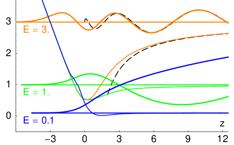

(right) Closed-channel or density modes , calculated perturbatively from the adiabatic approximation . We have shifted the potentials to so that the wave functions appear at the energy , as expected from Eq.(3); they have been multiplied by for better visibility. Dashed lines: simple adiabatic elimination .
In the adiabatic approximation (subscript ‘’), the equation for can be written in the form
| (20) |
where the potential is given by Eq.(17) for all (Fig.4(left)). At low energies, it is similar to the lower (blue) curve in Fig.2. We call it an ‘open channel’ because we have as so that is an extended wave right at the continuum threshold, with a turning point near , as shown in the Figure. B provides some details on the numerical calculation of these solutions.
Deep in the condensate, we find (black dashed line in Fig.4(left))
| (21) |
where the first term recovers the approximation (9). The ‘centripetal term’ arises from the first correction beyond the Thomas-Fermi approximation (the coefficient in Eq.(5)). The higher-order corrections arise from the next-to-leading order expansion of the root and from the geometric potential . The Schrödinger equation for therefore matches asymptotically with a modified Coulomb problem:
| (22) | |||
an equation that replaces Eq.(9) obtained above with a simpler argument. The required solutions are located just at the dissociation threshold of the Coulomb potential; they are known analytically and are linear combinations of Bessel functions (Abramowitz and Stegun, 1972) (black dashed in Fig.4(left))
| (23) |
The argument of the Bessel functions is familiar from the phase of the WKB solutions in Eq.(10). We have chosen a normalisation such that both Bessel-Coulomb solutions have the same amplitude deep in the condensate and their Wronskian is equal to unity (Abramowitz and Stegun, 1972)
| (24) |
Deep in the condensate, the Bogoliubov mode can therefore be represented in the form
| (25) |
where is a normalisation. This formula defines the phase shift of the Bogoliubov mode: the reference case corresponds to the Coulomb wave which is regular when extrapolated back to the condensate border (at in the Thomas-Fermi approximation). According to the asymptotic series of , , the Bogoliubov mode function will match the behaviour deep in the condensate we required in Eq.(11) above:
| (26) |
provided we choose the normalisation factor in Eq.(25) (see A, Eq.(71)). We recall that in this limit and that in the adiabatic approximation.
Note that the ‘centripetal potential’ that arises from the first ‘post-Thomas-Fermi’ correction in Eq.(5) is significant in this context. Dropping it from Eq.(22), the analytical solutions would involve first-order Bessel functions , which are phase-shifted by relative to their zeroth-order counterparts. This could have been expected from the long-range character of the centripetal potential, on the one hand. On the other, it is interesting to realise that one needs the function in Eq.(23) to recover the correct behaviour of the Bogoliubov modes at low energies, as required by the U(1) global phase symmetry of the mean field theory. We discuss the low-energy limit in more detail in Sec.2.4.
2.3 Non-adiabatic coupling and density modes in closed potential
We now take into account the off-diagonal (coupling) terms in the BdG equations and solve Eq.(15) for the density mode
| (27) |
This mode influences significantly the scattering phase shift , as we discuss in a companion paper (Diallo and Henkel, 2015). In addition, it also contributes to the spectrum of density fluctuations (dynamical structure factor), as illustrated in Sec.3.3 below.
The Schrödinger operator on the left-hand side of Eq.(27) corresponds to a wedge-shaped potential well whose minimum is above zero (Fig.4(right)). If the right-hand side is neglected, we therefore do not have any physically acceptable solution that remains finite for . Numerically, the inhomogeneous equation can be solved straightforwardly by representing the second derivative with a finite difference scheme and solving the corresponding sparse linear system. The results are shown in Fig.4(right) and Fig.5(left). As expected, the density mode is localised in the border region and has an amplitude much smaller than the phase mode. The ‘local approximation’ (gray dashed line) captures well its tails, but not the reduced amplitude of the oscillatory features (where the second derivative is obviously significant).
Some insight into the inhomogeneous Schrödinger Eq.(27) may be gathered by considering first the eigenvalue problem
| (28) |
for the potential well provided by . The eigenmodes provide a convenient basis to expand :
| (29) |
The coefficients are found by projecting Eq.(27) onto , using the natural scalar product
| (30) |
and choosing the normalisation . We get after two partial integrations
| (31) |
One key property here is that the source term in Eq.(27), , is actually a localised function (Fig.5(left), thick blue) because the differential operator involves the derivatives and that tend to zero as (see Eq.(19)). The matrix elements in Eq.(31) are therefore given by convergent integrals.
|
 |


(right) Squared norm (Eq.(32)) of the density mode as a function of energy (upper thick line). This is compared to the squares (Eq.(31)) of its expansion into low-lying trapped modes (thin lines, odd modes dashed). At the marked energies, the overlap to the ground mode is maximal and minimal, as shown in the left column.
The ‘trapped modes’ are illustrated in Fig.5(left). The closed-channel potential is harmonic only in a narrow range around its minimum. Hence, the spectrum is non-equidistant due to the linear asymptotes away from the minimum. We derive in C the asymptotics .
Pseudo-Feshbach resonance.
The results for the trapped density mode are summarised in Fig.5(right) where we plot the norm of the density mode (defined as in Eq.(32) below) vs. the energy . To interpret the oscillating features, we suggest an analogy to the so-called Feshbach resonances in atomic and molecular scattering. The physics is essentially the same: due to non-adiabaticity, different potential surfaces are coupled. The colliding system may thus split up and follow different paths which eventually interfere in the output (Stückelberg oscillations). A particularly strong effect occurs when a localised eigenstate in a closed channel becomes degenerate with the incoming wave in an open channel. In ultracold collisions, this mechanism operates when a differential Zeeman shift brings coupled spin states into resonance; the result is a divergence of the scattering length for specific values of the magnetic field (Feshbach resonance).
In our problem, we also have two potentials, open () and closed (). But there is no tuning parameter available to bring the initial wave into resonance with the closed-channel eigenvalues: the denominators in the amplitudes (Eq.(31)) never cross zero. One can even derive the stronger bound from the ground state of the harmonic approximation to the Hartree-Fock potential contained in (see Eq.(7)). There is, however, one possibility for a resonantly enhanced density mode. It is not related to a matching of energies, but of wave functions. Indeed, for the energy , one observes a quite accurate matching in shape and position between and the ground state (Fig.5(top left)). This leads (as in a Franck–Condon argument) to the strong peak in the norm of the density mode
| (32) |
as can be seen in Fig.5(right) where the probabilities are plotted as a function of energy and compared to the norm . A resonance with the first excited state at is visible because at a slightly lower energy (Fig.5(bottom left)), becomes orthogonal to the ground state . At this ‘anti-resonance’, the derivative term in is significant.
We have observed that the shape of the closed-channel potential is relatively stable as the energy increases (compare Fig.5(left, top and bottom)). The overlap therefore changes chiefly because the turning point and the nodes of the open-channel solution shift with , as we saw in Fig.4(left). The other reason is the shifting and broadening of the non-adiabatic couplings , that are involved in the operator (recall Fig.3).
2.4 Low-energy behaviour
It is well known that when the Bogoliubov spectrum is continuous, it is gapless and that the amplitudes and approach the shape of the condensate in the limit . This translates the Goldstone mode arising from the global phase invariance (U(1) symmetry) of the Gross-Pitaevskii equation (2). In this low-energy limit, the phase-density representation of Eqs.(8) becomes exact. For the sake of simplicity, we stay in the adiabatic basis (12) and get in the leading order the BdG equation for the phase mode
| (33) |
This is solved by the condensate itself. (For an illustration, see the curve in Fig.4(left).) In the same limit, there is only the trivial solution for the density mode. We fix the normalisation by continuity with the low-energy limit of the Bessel-Coulomb wave that is proportional to the Thomas-Fermi condensate:
| (43) |
We indeed find that the phase shift is very small in this limit so that the other Bessel-Coulomb wave (see Eq.(25)) has negligible weight at low energies (Diallo and Henkel, 2015). The spatial range where this behaviour is relevant opens up wide for .
3 Applications
3.1 Equilibrium correlations
It is well known that the Bogoliubov–de Gennes modes provide a convenient expansion of the field operator
| (44) |
where the operators () create (annihilate) an elementary excitation with energy . We have assumed a c-number condensate (Bogoliubov shift) for simplicity and added the subscript to the mode functions for clarity. Since the inhomogeneous potential is ‘open’ on the dense side, the energy spectrum is continuous. (The integration measure arises from the normalisation of the , , see A.) In thermal equilibrium, we have and the Bose occupation number
| (45) |
because the expansion (44) provides a quadratic approximation of the second-quantised field Hamiltonian. The elementary excitations contribute even at zero temperature (‘depletion’) because of the operator that appears in Eq.(44). We focus in the following on low temperatures and leave aside the problem of ‘quasi-condensation’ and self-consistent mean-field theories in low dimensions; see for example Andersen et al. (2002); Al Khawaja et al. (2002); Mora and Castin (2003).
3.2 Field correlation spectrum
Matter-wave interference experiments are sensitive to the dynamic field correlation function
| (46) |
where the time dependence arises from in the Heisenberg picture. (Recall that we have set the zero of energy at the chemical potential.) Inserting Eq.(44) and taking , we get the well-known expression
| (47) |
|
 |


We show in Fig.6 a contour plot of two terms: the ‘particle spectrum’ and the ‘hole spectrum’ (with the energy scale flipped). We recognise in the upper left quadrant (particles outside the condensate) a straight nodal line (dash-dotted) that is characteristic for the Airy function . As the modes enter the condensate, the nodal lines shift to the pattern , the first few roots of the Bessel function (dashed). This approximation is based on the asymptotic form (11) and works well because the Bogoliubov phase shift is small: (see Diallo and Henkel (2015)).
At low energies (bright central region in Fig.6(right)), the spectra for both particles and holes converge to the same limit (see Eq.(43)) that is essentially given by the condensate density (see Sec.2.4). The occupation number in Eq.(47) thus leads to an infrared divergence of the average density . This has been regularised by introducing the quasi-condensate concept (Kagan et al., 2000; Andersen et al., 2002): the divergence mainly arises from phase fluctuations which can be subtracted. See the discussion of the density correlations below.
Returning to the hole mode (Fig.6(bottom left)), we see that it is confined to the dense region and follows similar nodal lines as as expected from the boundary condition Eq.(11). The contour plot provides a representation of the so-called depletion density
| (48) |
which is simply the zero-temperature limit of the non-condensate density in Eq.(47) (a measure of quantum fluctuations). We have checked that this integral matches in the dense region (i.e., ) with the corresponding result for a homogeneous system 11 1 A useful parametrisation for the Bogoliubov amplitudes in a homogeneous system is , with . The dispersion relation is . Therefore in the dense limit : . (local density approximation with constant condensate )
| (49) |
where the modes are labelled by the wave vector and the dispersion relation is approximately linear . The logarithmic infrared divergence can also be cured with suitable subtractions (Andersen et al., 2002; Al Khawaja et al., 2002; Mora and Castin, 2003).
3.3 Density fluctuation modes
As a second application, we consider the leading order Bogoliubov contribution to the dynamic density correlations
| (50) |
The curly brackets denote a symmetrised operator product for the particle density . Its average does not depend on time (see Eq.(47) for ). The expectation value is worked out using the Bogoliubov shift (44) and expressed in terms of the occupation numbers (45), using the Wick theorem (gaussian statistics). Our result is consistent with Eq.(52) of Eckart et al. (2008) and reads
| (51) |
where the first line involves the correlation function of Eq.(46) and the field commutator
| (52) | |||||
Due to the completeness relation of the BdG modes, this goes over into when (see A). In Eq.(51), we use the ‘sum mode function’
| (53) |
which is, by a property of the BdG equations, orthogonal to the condensate with respect to the scalar product (30). The ‘4th order terms’ of the last line arise from products of four Bogoliubov operators and . Note that the second line features, for , an integral that is similar to infrared-regularised thermal densities introduced by Andersen et al. (2002); Al Khawaja et al. (2002); Mora and Castin (2003). This illustrates the consistency of these procedures, since their goal is to eliminate from the density spurious contributions attributed to phase fluctuations.


We focus for illustration purposes on the ‘beating’ between the condensate and the elementary excitations and show in Fig.7 the local spectrum
| (54) |
We find this formula by including the part of the first line in Eq.(51) that is proportional to the condensate density. The contour plot shows that the density fluctuations are peaking near the condensate border. This is as expected because deep inside a (quasi)condensate, such fluctuations are penalised by the self-interaction energy.
The density fluctuation spectrum does not show any infrared divergence because for small , the sum mode behaves proportional to (adiabatic angle in Eq.(12))
| (55) |
The scaling linear in at finite temperature can be seen in Fig.7(right). This plot also illustrates that the ‘trapped mode’ which is localised near the border (Fig.4(right)), gives a significant contribution (compare dashed and solid lines in Fig.7(right)). The comparison yields the interesting result that the beating between this mode and the condensate is actually reducing rather than enhancing low-frequency density fluctuations (set of lower curves for ).
4 Conclusion
The elementary excitations of a Bose condensate (Bogoliubov spectrum) are well-known in a homogeneous system (Pitaevskii and Stringari, 2003) and also within some approximations for a harmonically trapped gas (Al Khawaja et al., 2002; Stringari, 1996; Öhberg et al., 1997; Stringari, 1998). We have analysed in this paper the border region where the condensate density smoothly goes to zero, providing a detailed look at the physics beyond the Thomas-Fermi approximation. Previous work has focused on the condensate kinetic energy (Dalfovo et al., 1996; Lundh et al., 1997), ignoring the contribution of elementary excitation, and on the stability with respect to vortex formation, taking into account motion parallel to the border of the condensate (Lundh et al., 1997; Anglin, 2001). The mode functions provided here typically extend into the bulk of the condensate and would correspond in a three-dimensional isotropic trap to radially symmetric (angular momentum ) modes. Our main result is that the gradient in the condensate density couples elementary excitations that are mainly ‘phase-like’ and ‘density-like’, an effect clearly beyond the local-density approximation. This leads to density fluctuation modes that are localised near the border of the condensate. These fluctuations may be detected with scattering experiments using a focused probe beam that probe the dynamic structure factor locally, similar to the setup of Onofrio et al. (2000). Alternatively, one may directly analyse density-density correlations when an elongated system is imaged. This may be complemented by launching, with a suitable pulse sequence, an elementary excitation coming from the bulk (dense quasi-condensate), similar to the suggestion of Brunello et al. (2000). We also believe that the methods developed here provide a stepping stone towards a self-consistent description of an inhomogeneous Bose gas at finite temperature, using for example the modified Popov theory of Andersen et al. (2002) or the Bogoliubov theory for quasi-condensates of Mora and Castin (2003). The border region where the density drops is particularly interesting here because of the possibility of entering a strongly correlated phase, see for example Trebbia et al. (2006); Jacqmin et al. (2011), and Vogler et al. (2013).
Acknowledgements.
This work has been supported by a final-year student grant awarded to A.D by Universität Potsdam.
Appendix A Wronskians and normalisation
We start by a generalisation of the Wronskian for the BdG problem (two coupled equations). Our proposed definition is
| (56) |
where the prime denotes the first derivative. We assume that all modes including the condensate are real. The advantage of this combination are the following manipulations that can be applied to the pair of BdG equations
| (57) | |||||
| (58) |
where is the Hartree-Fock potential. Consider another pair of solutions , that solves the same equations with energy eigenvalue . Multiply Eq.(57) with , and Eq.(58) with , take the sum, and subtract the corresponding equation for multiplied by etc. On the left-hand side, we get , proportional to the integrand of the generalised -scalar product in the BdG space. On the right-hand side, we find the derivative of the Wronskian : the Hartree potential drops out as in the Schrödinger equation; also the coupling terms involving the condensate are cancelled: . Integrating and using the boundary conditions (4) for , we get
| (59) |
In other words: the scalar product can be analyzed locally from the asymptotic behavior of the mode functions. The orthogonality between modes with different energies in the discrete spectrum follows immediately (the Wronskian vanishes at both ends).
We continue by analyzing the continuous spectrum for the linear potential. Recall the asymptotic form deep in the condensate from Eq.(11):
| (60) |
and similarly for with amplitude . In this limit, the two amplitudes are given by the rotation back from the adiabatic basis
| (66) |
where we have used that only the adiabatic mode ‘survives’ and has amplitude . ( is localised in the Hartree-Fock-like well near the border, see Fig.4(right).) The scattering phase is therefore the same for both modes and . Similar amplitudes and apply for the other solution at energy . The Wronskian then becomes (denoting and similarly for )
| (67) |
Contributions from the derivatives would vanish like relative to this term, see Eq.(19). It is natural to interpret this as distribution with respect to the energies , to be put under an integral. The trigonometric functions can be re-written into , this gives the expression
| (68) |
Since both energies are positive, this is an oscillating function as . It averages to zero if integrated over some interval and therefore vanishes in the distribution sense. The Wronskian is thus given by the phase difference term
| (69) |
where we recognised in the last fraction an oscillatory representation of a -function
| (70) |
and used the continuity in energy of the phase shift and of the amplitudes. The latter sum to and in Eq.(11), we chose the normalisation . This leads from Eq.(59) to the orthogonality
| (71) |
which is the main result of this appendix. The symmetry transformation and of the BdG problem (57, 58) gives the additional orthogonality relation
| (72) |
As a consequence, we can easily check that the equations
| (73) |
translate the standard commutation relation of the field operator into an implementation of the canonical commutation relations for the elementary mode operators
| (74) |
provided the mode functions and are normalised as in Eq.(60) with . The Bogoliubov shift (condensate in Eq.(44)) does not change this conclusion. For a discussion of the zero mode in the BdG problem and the corresponding operators, see for example Mora and Castin (2003).
Appendix B Solving the BdG equations numerically
We use a standard differential equation solver for the Painlevé transcendent (Gross-Pitaevskii equation (2)). The solution that connects to the Thomas-Fermi profile is actually numerically unstable, and we match it around with the asymptotic expansion (5), keeping typically three terms.
To solve the BdG equation (14) in the open channel (mode ) in the adiabatic approximation, a standard forward solver is used: initialise with the tunnelling asymptote (4) and check that the potential is linear there. Integrate forward until a position and match to a solution of the modified Coulomb problem (22)
| (75) |
The coefficients are conveniently calculated with the help of the Wronskians
| (76) |
using the normalised Bessel-Coulomb solutions defined in Eq.(23).
At the position , the open potential may not yet have reached its Coulomb asymptote (see Eq.(21)), therefore the coefficients are still slowly varying. The Wronskians (76) satisfy a first-order differential equation that can be derived using the procedure explained after Eq.(58). This yields, for example,
| (77) |
We choose the position such that the following approximation to the open potential is accurate enough
| (78) |
This term arises from the expansion of the root ; other contributions (post-Thomas-Fermi correction, geometric potential) are smaller. We find that for , the relative error is smaller than for a wide range of energies. We compute the integral (77) numerically with the approximation (75) for . It converges because the potential difference scales like . One can avoid the evaluation of oscillatory Bessel functions for large arguments by (i) using their asymptotic form and (ii) shifting the integration contour into the complex plane after some point on the real axis. In this way, one is keeping clear of the branch cut of Eq.(78) at . This procedure now yields the extrapolated coefficients . The normalisation factor for the wave function is then , and the scattering phase shift follows from .
The calculation of the density mode is based on the adiabatic approximation for the inhomogeneous Schrödinger equation (15). We represent the differential operator in the closed potential on a grid with a finite difference scheme. The size of the grid is adapted to the support of the source term . Due to the nonzero minimum of the potential, zero energy is not in the spectrum of the differential operator, hence the inhomogeneous equation is solved by a straightforward matrix inversion.
Appendix C Trapped states
The closed potential has linear asymptotes on both sides (see its Thomas-Fermi approximation in Eqs.(81, 82) below). Physically allowed eigenmodes therefore join into tunnelling solutions and occur only for discrete eigenvalues (see Eq.(28), not to be confused with which remains a continuous parameter).

For the numerical calculation of the trapped states in the closed potential, we use the finite-difference scheme of the preceding B and take a standard sparse eigenvector solver. Examples are shown in Fig.5(left column). A comparison of the spectrum with the familiar Bohr-Sommerfeld quantisation rule is given in Fig.8. Recall that this rule is based on the action integral
| (79) |
where are the left and right roots of (also known as turning points). The phase arises from the Langer correction at both turning points (Messiah, 1995). The eigenvalues are then approximately given by
| (80) |
The action integral, computed numerically, is plotted as thick lines in Fig.8, and a good agreement with the numerically computed eigenvalues is found. For the plot, the colored squares mark the pair . To enhance the difference, we have subtracted the leading term from the action, see Eq.(83) below.
The dashed lines in the figure show the Thomas-Fermi approximation to the action that can be computed analytically and provides a relatively accurate estimate. The closed potential is approximated by
| (81) | |||||
| (82) |
These formulas are also useful to estimate the position of the left and right turning points . The action integral gives from the region , and the range can be evaluated with the substitution . Summing the two, we get
| (83) | |||||
The first two terms give with the Bohr-Sommerfeld rule (80) the eigenvalue spectrum mentioned after Eq.(31). The scaling law illustrates the non-equidistant spectrum in this anharmonic well. Eq.(83) captures relatively well the numerically computed action (compare dashed and solid lines in Fig.8), except at low energies where the Thomas-Fermi approximation fails to reproduce the shape of the potential.
References
- Ablowitz and Segur (1977) Ablowitz, M. J., Segur, H., 1977. Exact linearization of a Painlevé transcendent. Phys. Rev. Lett. 38 (20), 1103–06.
- Abramowitz and Stegun (1972) Abramowitz, M., Stegun, I. A. (Eds.), 1972. Handbook of Mathematical Functions, ninth Edition. Dover Publications, Inc., New York.
- Al Khawaja et al. (2002) Al Khawaja, U., Andersen, J. O., Proukakis, N. P., Stoof, H. T. C., 2002. Low dimensional Bose gases. Phys. Rev. A 66, 013615, erratum: Phys. Rev. A 66, 059902(E) (2002).
- Andersen et al. (2002) Andersen, J. O., Khawaja, U. A., Stoof, H. T. C., 2002. Phase fluctuations in atomic Bose gases. Phys. Rev. Lett. 88, 070407.
- Anglin (2001) Anglin, J. R., 2001. Local vortex generation and the surface mode spectrum of large Bose-Einstein condensates. Phys. Rev. Lett. 87, 240401.
- Berry (1984) Berry, M. V., 1984. Quantal phase factors accompanying adiabatic changes. Proc. R. Soc. London A 392, 45–57.
- Brunello et al. (2000) Brunello, A., Dalfovo, F., Pitaevskii, L., Stringari, S., 2000. How to measure the Bogoliubov quasiparticle amplitudes in a trapped condensate. Phys. Rev. Lett. 85 (21), 4422–25.
- Dalfovo et al. (1996) Dalfovo, F., Pitaevskii, L., Stringari, S., 1996. Order parameter at the boundary of a trapped Bose gas. Phys. Rev. A 54 (5), 4213–17.
- Diallo and Henkel (2015) Diallo, A., Henkel, C., 2015. Bogoliubov phase shifts at a nonlinear turning point, in preparation.
- Eckart et al. (2008) Eckart, M., Walser, R., Schleich, W. P., 2008. Exploring the growth of correlations in a quasi one-dimensional trapped Bose gas. New J. Phys. 10, 045024, eq.(52) corrects a typographic error in Eq.(91) of Walser (2004).
- Egorov et al. (2011) Egorov, M., Ivannikov, V., Opanchuk, B., Hall, B. V., Hannaford, P., Sidorov, A. I., 2011. Precision measurements of s-wave scattering lengths in a two-component Bose-Einstein condensate. In: Proceedings of the International Quantum Electronics Conference and Conference on Lasers and Electro-Optics Pacific Rim 2011. Optical Society of America, p. I1034, see also arXiv:1205.1591.
- Fetter and Feder (1998) Fetter, A. L., Feder, D. L., 1998. Beyond the Thomas-Fermi approximation for a trapped condensed Bose-Einstein gas. Phys. Rev. A 58 (4), 3185–94.
- Gross (1961) Gross, E. P., 1961. Structure of a quantized vortex in boson systems. Nuovo Cim. 20 (3), 454–76.
- Hastings and McLeod (1980) Hastings, S., McLeod, J., 1980. A boundary value problem associated with the second Painlevé transcendent and the Korteweg-de Vries equation. Arch. Rational Mech. Anal. 73 (1), 31–51.
- Hyouguchi et al. (2002) Hyouguchi, T., Adachi, S., Ueda, M., 2002. Divergence-free WKB method. Phys. Rev. Lett. 88, 170404.
- Jacqmin et al. (2011) Jacqmin, T., Armijo, J., Berrada, T., Kheruntsyan, K. V., Bouchoule, I., 2011. Sub-poissonian fluctuations in a 1D Bose gas: From the quantum quasicondensate to the strongly interacting regime. Phys. Rev. Lett. 106, 230405.
- Kagan et al. (2000) Kagan, Y., Kashurnikov, V. A., Krasavin, A. V., Prokof’ev, N. V., Svistunov, B., 2000. Quasicondensation in a two-dimensional interacting Bose gas. Phys. Rev. A 61, 043608.
- Langer (1937) Langer, R. E., 1937. On the connection formulas and the solutions of the wave equation. Phys. Rev. 51, 669–76.
- Lifshitz and Pitaevskii (1980) Lifshitz, E. M., Pitaevskii, L. P., 1980. Statistical Physics (Part 2), 2nd Edition. Vol. 9 of Landau and Lifshitz, Course of Theoretical Physics. Pergamon, Oxford.
- Lundh et al. (1997) Lundh, E., Pethick, C. J., Smith, H., 1997. Zero-temperature properties of a trapped Bose-condensed gas: Beyond the Thomas-Fermi approximation. Phys. Rev. A 55 (3), 2126–31.
- Margetis (2000) Margetis, D., 2000. Asymptotic formula for the condensate wave function of a trapped Bose gas. Phys. Rev. A 61, 055601.
- Messiah (1995) Messiah, A., 1995. Mécanique quantique, nouvelle Edition. Vol. I. Dunod, Paris.
- Mora and Castin (2003) Mora, C., Castin, Y., 2003. Extension of Bogoliubov theory to quasicondensates. Phys. Rev. A 67 (5), 053615.
- Öhberg et al. (1997) Öhberg, P., Surkov, E. L., Tittonen, I., Stenholm, S., Wilkens, M., Shlyapnikov, G. V., 1997. Low-energy elementary excitations of a trapped Bose-condensed gas. Phys. Rev. A 56 (5), R3346–49.
- Onofrio et al. (2000) Onofrio, R., Durfee, D. S., Raman, C., Köhl, M., Kuklewicz, C. E., Ketterle, W., 2000. Surface excitations of a Bose-Einstein condensate. Phys. Rev. Lett. 84 (5), 810–13.
- Pitaevskii (1961) Pitaevskii, L. P., 1961. Vortex lines in an imperfect Bose gas. J. Eksp. Teor. Fiz. 40, 646–51, [Sov. Phys. JETP 13 (2), 451–54 (1961)].
- Pitaevskii and Stringari (2003) Pitaevskii, L. P., Stringari, S., 2003. Bose-Einstein Condensation. Vol. 116 of International Series of Monographs on Physics. Oxford University Press, Oxford New York.
- Stringari (1996) Stringari, S., 1996. Collective excitations of a trapped Bose-condensed gas. Phys. Rev. Lett. 77, 2360.
- Stringari (1998) Stringari, S., 1998. Dynamics of Bose-Einstein condensed gases in highly deformed traps. Phys. Rev. A 58 (3), 2385–88.
- Trebbia et al. (2006) Trebbia, J.-B., Esteve, J., Westbrook, C. I., Bouchoule, I., 2006. Experimental evidence for the breakdown of a Hartree-Fock approach in a weakly interacting Bose gas. Phys. Rev. Lett. 97, 250403.
- Vogler et al. (2013) Vogler, A., Labouvie, R., Stubenrauch, F., Barontini, G., Guarrera, V., Ott, H., 2013. Thermodynamics of strongly correlated one-dimensional Bose gases. Phys. Rev. A 88 (3), 031603.
- Walser (2004) Walser, R., 2004. Ground state correlations in a trapped quasi one-dimensional Bose gas. Opt. Commun. 243 (1-6), 107–29.
- Wilczek and Shapere (1989) Wilczek, F., Shapere, A. (Eds.), 1989. Geometric Phases in Physics. Vol. 5 of Advanced Series in Mathematical Physics. World Scientific.